Revenue sharing contract for a VMI with one for one period policy

Abstract

In this article, we design a revenue-sharing contract to coordinate inventory control decisions in a serial supply chain consisting of one supplier, one vendor, and one retailer. We assume that the retailer faces Poisson demand and his unsatisfied demands will be lost. The retailer applies one-for-one period policy in which he constantly places an order for one unit of product to the vendor in a predetermined time interval which results in a deterministic demand for the vendor. Vendor orders the required quantity from supplier which will be immediately received at the vendor’s warehouse. Solution procedures are developed to find the equilibrium in the vendor managed inventory program with a revenue-sharing contract. Furthermore, we obtain the optimal order cycle for the retailer and the vendor which minimizes the supply chain’s total cost.

Keywords:

• revenue sharing contract
• supply chain management
• one-for-one period policy
• vendor managed inventory

PUBLIC INTEREST STATEMENT

There is always a complicated interactions in a supply chain between suppliers, vendors, and retailers. Each of these parties try to synchronize their demands and their orders in order to minimize the cost and maximize benefits. Situation might get more complicated when revenue would be shared between two or more parties. Our target is to devise an innovative and simple approach to this problem by controlling inventory control decisions between retailer and vendor and make retailer placing an order for one unit of product in a determined time interval. In this way, not only vendor would face a deterministic demand rate and hence could optimize its demands from the suppliers, but also the whole supply chain cost would be minimized. We also claim that we could find the optimal order cycle need to reach this minimal cost.

1. Introduction and literature review

Interaction between supply chain members has been extensively discussed before. There has been a vast body of work on centralized and decentralized inventory systems. Bernstein and Federgruen (2005) studied the equilibrium behavior of a decentralized supply chain with competing retailers under demand uncertainty. Cachon and Zipkin (1999) showed that efficiency is reduced when there is competition in a two-stage serial supply chain. They also established that the value of cooperation is context specific; in some settings competition increases the total cost by only a fraction of a percent, whereas in other settings the increasing in cost is enormous. Guan and Zhao (2010) formulated models to optimize sales volumes in a multiretailer system operated on an infinite time horizon with stochastic demands. Considering Cournot competition, they simultaneously optimized the expected sales volumes and (r, Q) policies for all retailers.

In the traditional supply chain, it is the retailer who controls his own inventory and places orders to the supplier. In vendor managed inventory (VMI) systems, it is the supplier who controls the retailers’ inventories and makes decisions on when and how to replenish them. In recent years, contract designs for VMI programs are recognized to be an important issue. Yu, Chu, and Chen (2009) studied a VMI system of a single manufacturer and multiple retailers and provided a solution for maximizing profits of both the manufacturer and retailers. Yu, Hong, Zhang, Liang, and Chu (2011) extended their work to find the best strategy to select retailers by providing a nonlinear, mixed-integer, game-theoretic, and analytically intractable Stackelberg game model to help the vendor to optimally select his retailers.

Capacity-constrained manufacturer in a VMI system was the focus of study in Almehdawe and Mantin (2009). They compared dominance of retailers and the manufacturer and showed that the retailer dominance, in general, results in higher supply chain efficiency and the highest overall efficiency is when the leader has the lowest market scale among other retailers.

Mateen, Chatterjee, and Mitra (2015) provided formulations for minimizing the expected total cost for the VMI when overstocking is penalized. They also studied four different VMI models in Mateen et al. (2015) and formulated the costs for different aspects of inventory synchronization such as replenishment policy and batch size in product delivery and showed that the all VMI models have less cost than retailer-controlled system. Within VMI models, the one which uses sub-batch size deliveries is proven to have less cost. While Hoque (2009) follows the same approach in his research, Hariga, Gumusb, and Daghfousb (2012) allow unequal shipments to retailers. Hariga, Gumus, Daghfous, and Goyal (2013) showed that taking equal replenishment intervals as the base solution, an algorithm could be devised to find a near-optimal solution for unequal intervals in an iterative approach.

Lee and Cho (2013) studied a VMI contract with (r, Q) policy and showed that although VMI may result in significant cost savings for both parties, the retailer may not always benefit from VMI, especially when the ratio of the supplier’s fixed cost to that of the retailer’s is small and/or when the physical storage cost is relatively large compared with the cost of capital.

In this paper, we focus on the contract design for VMI programs. In contrast, many papers study the design of contracts for non-VMI modes, for example, retailer managed inventory, or RMI for short. For instance, Krichen, Laabidi, and Ben Abdelaziz (2009) discussed a retailer-managed inventory system in which supplier proposes discounts and delay in payments based on the quantity of orders. They proposed a decision rule that generates preferred coalitions for each retailer to reduce the number of explored coalition structures. In some papers, the supply chain efficiency has been studied under different inventory management structures. Govindan (2012) compared VMI and non-VMI systems using pharmaceutical industry data and showed that the VMI system performs better than non-VMI system.

In order to satisfy customers’ heightened expectations, the enterprises increasingly find that they must rely on effective supply chains. A nonefficient supply chain may carry a high cost. Consequently, supply chain performance largely depends on the coordination of materials, information, and financial flows of several separated firms. The supply chain members are autonomous and primarily concerned with optimizing their own objectives. This self-interest may result in poor performance. In order to align each member’s objective with the supply chain’s objective, contracting is a way to coordinate supply chain members such that optimal performance is achievable. Contract characterizes the information and financial flow and specifies the duties and rights of each member which coordinate contractual members by set of transfer payments. In the research literature on supply chain management, coordination issues have attracted an extensive research. Some researchers have studied coordination problem by contract.

Since video cassette rental issues were raised by BlockBuster, Inc., revenue sharing contracts have come to spotlight. Providing a contract for sharing profits between retailers and vendors changes the inventory parameters drastically. Cachon and Lariviere (2005) comprehensively investigate the use of revenue sharing for coordination of the distribution channel. They show that revenue-sharing makes the retailer to choose optimal actions for the supply chain (quantity and price) and distributes the channel profits between the supplier and the retailer. Kunter (2010) showed that channel coordination requires sharing of cost and revenue via a sharing rate and marketing effort participation on both manufacturer and retailer level. Also, efficiency requires that a retailer’s participation of at least 50% in the manufacturer’s cost of marketing effort. Wang, Jiang, and Shen (2004) showed that under a revenue sharing contract between a supplier and a vendor in which supplier decides on the retail price and delivery quantity for this product, both channel performance and the performance of individual firm depend critically on demand price elasticity and on the retailer’s share of channel cost. Yao, Leung, and Lai (2007) showed that in case of competitive retailers, the provision of revenue-sharing in the contract can obtain better performance than a price-only contract. Liu, Xu, and Kouhpaenejad (2010) provided a non-linear programming model for solving the fairest revenue-sharing coefficients between logistic service integrator and functional service provider when they have stochastic demand condition. Palsule-Desai (2011) compared revenue-dependent revenue-sharing contracts with revenue-independent revenue-sharing contracts and showed that there exist situations in which revenue-dependent contracts outperform revenue-independent contracts. El Ouardighi (2014) extended the revenue-sharing idea to collaboration of manufacturer and supplier to improve the quality of the product. Chakraborty, Chauhan, and Vidyarthi (2013) studied comparing revenue-sharing contracts with wholesale price in common retailer channel and deduced that when common retailer has the lead role, it is beneficial for retailer to offer salvage revenue-sharing contract. When manufacturers are leaders, then it is beneficial for the manufacturers to offer wholesale price contract although revenue-sharing contract improves the channel performance. Zhang, Liu, Zhang, and Bai (2014) focused on how to improve the efficiency of a supply chain for deteriorating items with a revenue sharing and cooperative investment contract. Guan and Zhao (2010) showed that in a VMI system with (r, Q) policy, when there is a franchising contract for retailer with ownership, the system achieves the same performance as in centralized control.

In addition to the supply chain structure and the kind of interactions and coordination between supply chain members, the replenishment policy also has significant impact on supply chain efficiency. In many cases, by choosing appropriate combination of replenishment policy and coordination mechanism we can increase supply chain efficiency tremendously and even in some cases it will lead to perfect coordination. Supply chain environmental conditions such as demand function, shortage type and the cost functions are some substantial parameters for each member to choose the suitable inventory policy.

Finding replenishment policy for the supply chain in which the unsatisfied demand lost is studied by a few papers. Bijvank and Vis (2009) reviewed and classified review policies for lost-sales inventory system and deduced that for continuous reviews, comparing (s, Q) policies, (S-1, S) policies and (s, S) policies, most of the work has been done so far was on (s, Q); although still not much is known about an optimal replenishment policy when excess demand is lost. Andersson and Melchiors (1999) proposed a heuristic algorithm for cost-effective base-stock policy to prevent stock outs when both warehouse and all retailers use (S-1, S) review policy. They showed that the cost of the policies is just 0.4% above optimal policy. Seifbarghy and Akbari Jokar (2005) developed an approximate cost function to find the optimal reorder points for given batch sizes in all installations when retailers are working under continuous review inventory policy (r, Q).

While it is well known that for stochastic demand, there is no inventory control policy in which both the order size and the order interval are constant with an optimal solution, Haji and Haji (2007) and later Haji, Pirayesh Neghab, and Baboli (2006) proposed a new One-for-One period policy, in which one unit of product is ordered in each ordering period and so eliminating uncertainty in demand for suppliers. They derived the long-run average total inventory cost, including holding and shortage costs in terms of the average inventory and showed that their cost function has a unique solution. They also formulated the optimal value of the time interval between two consecutive orders. As discussed in Haji and Haji (2007), for the one for one period policy, an order for one unit of item is placed in a predetermined time interval. Hence, both the order size and the order interval are constant. As such, this policy prevents expanding the demand uncertainty for supplier. That is, the demand for the supplier is deterministic, one unit every $T$ units of time.

In our study, we consider a supply chain consisting of a single vendor and a single retailer facing stochastic demand. The ordering cost of the retailer is negligible and the retailer uses one-for-one period ordering $\left(1,T\right)$ policy. We design a revenue sharing contract for the VMI program to improve the supply chain efficiency and minimize its total inventory cost. We formulate the centralized control and the VMI program of a serial supply chain consisting of a supplier, a vendor and a retailer. We show that the revenue sharing contract will lead to perfect coordination of the supply chain.

2. Problem statement

We study a revenue sharing contract and its further improvement for a serial supply chain consisting of a supplier, a vendor, and a retailer as shown in Figure 1.

Figure 1. A serial supply chain consisting of a supplier, a vendor, and a retailer.

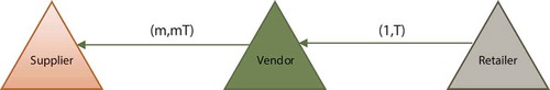
The retailer uses a new ordering policy called one-for-one period ordering $\left(1,T\right)$ policy developed by Haji et al. (2007) in which an order of size one is placed at every fixed cycle time $T$. This policy results in a deterministic demand for the vendor. The vendor must obtain the optimum ordering times of the retailer and his own to satisfy the orders of retailer. That is, at every $T$ units of time, he delivers 1 unit of the product to the retailer and at every $mT$ units of time, he places an order (of size $m$) to the outside supplier. Furthermore, since the lead time to the vendor from the outside supplier is constant, to further reduce his holding cost due to satisfying the retailer’s orders, he places his orders to outside supplier in such a way that the arrival times of the orders coincide with the arrival times of the retailer’s orders.

2.1. Assumptions

The research problem can be defined by the following assumptions:

1. The fixed ordering cost is zero or negligible at the retailor.

2. The demand process is Poisson and unsatisfied demands will be lost at the retailer.

3. The replenishment lead time is constant both at the retailer and the vendor.

4. The transportation time of each order placed by the retailer is assumed to be constant.

5. Shortage is not allowed for the vendor.

6. The transportation time from the supplier to the vendor is constant and the supplier has enough stock that would never face shortages.

To satisfy the retailer’s demand, the vendor should determine times and quantities of his orders to supplier in a way that the retailer’s demand is satisfied on time and his total inventory cost is minimized.

To facilitate comparisons, we analyze the system performance in centralized control, which plays the role of benchmark. Then we will investigate coordination of the supply chain through a revenue sharing contract in a VMI program in which the retailer agrees to give a percentage of his revenue to the vendor. Because the vendor is responsible for supply chain inventory levels and incurs the related costs from the fluctuations of these levels, the vendor decides about the inventory policy of the supply chain.

2.2. Notation

We introduce the following notations:

$\mu$:	=	Demand rate at the retailer
$p$:	=	The product sales price to customer
$\pi$:	=	Unit cost of a lost sale at the retailer
$h_r$:	=	Holding cost of a product unit during one period at the retailer
$T$:	=	Ordering cycle of the retailer
$I$:	=	Average inventory level at the retailer
$\mathrm{C}\mathrm{R}$:	=	Expected total cost per unit time for the retailer
$A$:	=	Ordering cost for the vendor
$h_v$:	=	Holding cost of a product unit during one period in vendor’s warehouse
$m$:	=	Integer value which determines the ordering cycle of the vendor to the supplier ($mT$)
$\phi$:	=	The percentage of the revenue the retailer keeps. The percentage ($1-\phi$) is delivered to the vendor. $\phi$ is determined through bargaining between the two parties, $\phi ϵ\left[0,1\right]$
CV:	=	Total vendor’s inventory cost per unit time
TC:	=	Total system cost per unit time, $\mathrm{T}\mathrm{C}=\mathrm{C}\mathrm{V}+\mathrm{C}\mathrm{R}$

3. Model formulation

3.1. Inventory cost of the retailer

The retailer uses a new ordering policy called one-for-one period ordering $\left(1,T\right)$ policy developed by Haji et al. (2007) in which an order of size one is placed at every fixed cycle time $T$. Hence, the inventory problem can be interpreted as a $D/M/1$, a single channel queuing system in which the inter-arrival times, $T$, are constant and the service times have exponential distribution with mean value of $1/\mu$. Thus, the arrival rate of units to the system is $\lambda =1/T$ and the service rate is $\mu$. According to their derivation the total cost at retailer $i$ is

(1) $\mathrm{C}\mathrm{R}=-p\mu \rho +h_{r}I+\pi \mu \left(1-\rho \right)$(1)

Where $\rho$ is the proportion of the demand satisfied by the retailer and $s\mu \rho$ is the revenue obtained by the retailer from selling the product. Also, $\left(1-\rho \right)$ is the proportion of time that the retailer is out of stock, as such, $\pi \mu \left(1-\rho \right)$ is his lost sales cost per unit time, since

(2) $\rho =\frac{\lambda }{\mu }=\frac{1}{T\mu }$(2)

Haji et al. (2007) also show that the average inventory is

(3) $I=\frac{\rho }{1-\beta }$(3)

Where

(4) $\beta =e^{-\frac{1-\beta }{\rho }}=e^{-\frac{1}{I}}$(4)

Consequently,

(5) $\rho =I\left(1-\beta \right)=I\left(1-e^{-\frac{1}{I}}\right)$(5)

So, we can represent average inventory cost of the retailer as follows:

(6) $\mathrm{C}\mathrm{R}=-p\mu I\left(1-e^{-\frac{1}{I}}\right)+h_{r}I+\pi \mu \left(1-I\left(1-e^{-\frac{1}{I}}\right)\right)$(6)

And we can find $T$ which minimizes the total cost as:

(7) $T=\frac{1}{\mu I\left(1-e^{-\frac{1}{I}}\right)}$(7)

3.2. Inventory cost of the vendor

The vendor receives orders from the retailer based on the optimal replenishment cycles. In this scenario, the retailer orders one unit of one type of product at specific intervals ($T$) to the vendor. In other words, order quantities are discrete and periodic. So, the vendor should decide on his ordering pattern (number, time, and quantity of his orders) to the supplier. As shortage is not allowed and the vendor avoids keeping excessive inventory, the vendor’s ordering quantities should be obtained at the ordering times of the retailer. Regarding the retailer’s ordering times and quantities, the vendor decides how often and how much to order to the supplier to minimize the holding and ordering costs besides fulfilling retailer’s demand without any shortage. So the vendor uses the integer-ratio policy (see also Guan & Xiaobo Zhao, 2009; Hariga et al., 2013; Mateen et al., 2015; Yu et al., 2009), in which the replenishment cycle of the vendor equals $mT$. In this inventory policy, the replenishment cycle of the vendor is $m$, an integer multiple of the common replenishment cycle ($T$).

To satisfy the retailer’s orders, the vendor should order $m$ units of the product in every $mT$ units of time to his supplier. So, the vendor should obtain the optimum value of $m$ to minimize the holding and ordering in the long term. The inventory level of the vendor by this policy is depicted in Figure 2.

Figure 2. The inventory level of the product at the vendor.

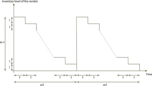
Then the inventory cost of the vendor based on his replenishment cycle $mT$ is

(8) $\mathrm{C}\mathrm{V}=\frac{h_v\left(m-1\right)}{2}+\frac{A}{mT}$(8)

By substituting (7) for $T$, we have

(9) $\mathrm{C}\mathrm{V}=\frac{h_v\left(m-1\right)}{2}+\frac{A\mu I\left(1-e^{-\frac{1}{I}}\right)}{m}$(9)

3.3. Centralized control

To facilitate the comparison, we analyze the system performance for the case of centralized control, which plays the role of a benchmark. From Equations (6) and (9) we can formulate the total inventory cost of the supply chain as follows:

(10) $\mathrm{T}\mathrm{C}=-p\mu I\left(1-e^{-\frac{1}{I}}\right)+h_{r}I+\pi \mu \left[1-I\left(1-e^{-\frac{1}{I}}\right)\right]+\frac{h_v\left(M-1\right)}{2}+\frac{A\mu I\left(1-e^{-\frac{1}{I}}\right)}{m}$(10)

We will use Theorems 1, 2, and 3 to investigate the properties of $I$ and $m$ for the optimal inventory policy which minimizes the supply chain cost. To achieve this purpose, we propose a convergence algorithm to find the optimal inventory policy for the supply chain in a centralized control environment.

Theorem 1: For any fixed $I$ the optimal $m$ can be uniquely determined by satisfying the following condition:

(11) $m^{\ast }\left(m^{\ast }-1\right)\le \frac{2A\mu I\left(1-e^{-\frac{1}{I}}\right)}{h_v}\le m^{\ast }\left(m^{\ast }+1\right)$(11)

Proof: see proof in Appendix A.

□

Theorem 2: The optimal value of $I$ (denoted as $I^{\ast }$) to minimize (10) has to satisfy

(12) $\frac{\mathrm{\partial }\mathrm{T}\mathrm{C}}{\mathrm{\partial }I}{|}_{I=I^{\ast }}=0$(12)

Proof: see proof in Appendix B.

□

By solving and simplifying Equation (12) we have

(13) $\frac{h_r}{\mu \left(\frac{A}{m}-\pi -p\right)}=-\left(1-e^{-\frac{1}{I^{\ast }}}-\frac{1}{I^{\ast }}{e}^{-\frac{1}{I^{\ast }}}\right)$(13)

The right-hand side of Equation (13) is always negative for all values of $I$. So, from Equation (13) we know that $\frac{A}{m}-\pi -p$ should be smaller than zero. Thus we can find the minimum value of $m$ as follow:

(14) $m_{min}=⌈\frac{A}{\pi +p}⌉$(14)

In which $⌈x⌉$ represents the least integer greater than or equal to $x$. Now that we have found a lower bound for the value of $m$ using Equation (14), by Theorem 3 we can show that the optimum value of $I$ is bounded.

Theorem 3: The optimal value of $I$ for Equation (13) is bounded.

Proof: See proof in Appendix C.

□

Using Theorems 1, 2, and 3, we have developed an enumerative algorithm to find the optimal inventory policy for the supply chain participating in centralized control policy. Then, we show that the algorithm is capable of finding the optimal solution in Theorem 4.

3.3.1. The algorithm for the case of centralized control

Now, the unique solution can be obtained by following Algorithm:

Algorithm 1: Find $m_{\mathrm{m}\mathrm{i}\mathrm{n}}$ from Equation (14). Calculate candidate solutions $I^{\ast }$ for $m=m_{\mathrm{m}\mathrm{i}\mathrm{n}},m_{\mathrm{m}\mathrm{i}\mathrm{n}}+1,m_{\mathrm{m}\mathrm{i}\mathrm{n}}+2,\dots$ separately by Equation (13) and for each $m$ check whether Equation (11) is satisfied. Once Equation (11) is satisfied, $m^{\ast }$ and $I^{\ast }$ are obtained. This enumerative method is feasible because $m$ is normally relatively small (<10 in practice).

Theorem 4: The algorithm 1 finds the unique optimal policy in the case of centralized control.

Proof: See proof in Appendix D.

□

3.4. Revenue sharing contract under VMI control

In this model we assume that the vendor controls the replenishment process of both parties and determines the optimal replenishment cycles of himself and the retailer. Hence, the vendor bears the expenses of his own setup cost $A$ per replenishment, his expected holding $h_v$ per time unit and expected holding cost of the retailer $h_R$ per time unit. The retailer receives an expected revenue per time unit and incurs an expected penalty cost for lost sales per time unit.

The retailer returns a percentage of sales revenue,$1-\phi$, to the vendor which is determined through bargaining between the two parties. When the vendor manages the inventory according to one-for-one period policy the resultant cost at the retailer is given by

(15) $\mathrm{C}\mathrm{R}=-\phi p\mu I\left(1-e^{-\frac{1}{I}}\right)+\pi \mu \left[1-I\left(1-e^{-\frac{1}{I}}\right)\right]$(15)

And the vendor’s inventory cost is

(16) $\mathrm{C}\mathrm{V}=-\left(1-\phi \right)p\mu I\left(1-e^{-\frac{1}{I}}\right)+h_{r}I+\frac{h_v\left(m-1\right)}{2}+\frac{A\mu I\left(1-e^{-\frac{1}{I}}\right)}{m}$(16)

From Equations (15) and (16) the system cost is then

(17) $\mathrm{T}\mathrm{C}=-p\mu I\left(1-e^{-\frac{1}{I}}\right)+h_{r}I+\pi \mu \left[1-I\left(1-e^{-\frac{1}{I}}\right)\right]+\frac{h_v\left(m-1\right)}{2}+\frac{A\mu I\left(1-e^{-\frac{1}{I}}\right)}{m}$(17)

It is seen from Equation (17) that the proportion $\phi$ does not influence the system cost.

The vendor hopes for the replenishment policy to minimize (16), which includes the setup cost and the holding cost, whereas the retailer prefers the replenishment policy that generates lower penalty cost in (15).

Like the centralized supply chain in Section 3.3, there are some considerations for the optimal solution in VMI program which have been presented in Theorems 5 and 6. We have used these theorems to develop a convergent algorithm to find the optimal inventory policy in VMI program with revenue sharing contract.

Theorem 5: The optimal value of $I$ (denoted as $\tilde{I}$) to minimize (16) is to satisfy

(18) ${\left.\frac{\mathrm{\partial }\mathrm{C}\mathrm{V}}{\mathrm{\partial }I}\right|}_{I=\tilde{I}}=0$(18)

Proof: See proof in Appendix E.

By solving and simplifying Equation (18), we have

(19) $\frac{h_r}{\mu \left(\frac{A}{m}-\left(1-\phi \right)p\right)}=-\left(1-e^{-\frac{1}{I^{\ast }}}-\frac{1}{I^{\ast }}{e}^{-\frac{1}{I^{\ast }}}\right)$(19)

The right-hand side of Equation (19) is always negative for all values of $I$. So, from Equation (19) we know that $\frac{A}{m}-\left(1-\phi \right)p$ should be smaller than zero. Thus, we can find the minimum value of $m$ as follows:

(20) $m_{\mathrm{m}\mathrm{i}\mathrm{n}}=\frac{A}{\left(1-\phi \right)p}$(20)

Now that, we have found a lower bound for value of $m$ using Equation (20), by Theorem 6 we can show that the optimum value of $I$ is bounded as follow.

Theorem 6: The optimal value of $I$ for Equation (19) is bounded.

Proof: See proof in Appendix F.

Although the vendor possesses the priority to determine the optimal policy, he needs the retailer to cooperate to determine the policy. So, the proportion $\phi$ and the value of expected inventory level $I$ are determined by both parties through the following algorithm.

3.5. Algorithm 2 (revenue sharing contract)

Step 1: The negotiation starts at ${\phi }_{\mathrm{m}\mathrm{a}\mathrm{x}}$, which is the maximum revenue sharing coefficient accepted by the two parties to enter the VMI program. In other words, $(1-{\phi }_{\mathrm{m}\mathrm{a}\mathrm{x}})$ is the minimum revenue share the retailer will give to the vendor to manage his inventory. The vendor determines the optimal values of $I$ and $m$ which minimize Equation (16) denoted by $\left(\tilde{I},\tilde{m}\right)$. The vendor then presents the policy to the retailer. The retailer finds his cost $\mathrm{C}\mathrm{R}$ according to Equation (15). Since the vendor handles inventory cost and does not consider shortage cost in determining the optimal inventory level, the value of $\tilde{I}$ will be smaller than $I^{\ast }$ in centralized control. Consequently, system cost $\mathrm{T}\mathrm{C}=\mathrm{C}\mathrm{V}+\mathrm{C}\mathrm{R}$ should be relatively high due to a small value of $I$.

Step 2: The retailer desires to increase the inventory level to gain more profit, so in negotiations he tries to increase $I$, which leads to an increase in $\mathrm{C}\mathrm{V}$ and a reduction of $\mathrm{C}\mathrm{R}$. Provided $\mathrm{T}\mathrm{C}=CV+\mathrm{C}\mathrm{R}$ is reduced, both parties can benefit as a win–win result by appropriately modifying $\phi$. The procedure repeats until $\mathrm{T}\mathrm{C}$ becomes increasing, wherein an equilibrium is reached. The resultant policy at the equilibrium is denoted by $\left({\phi }^{\ast },I^{\ast \ast },m^{\ast \ast }\right)$.

Step 3: Find the solution and stop. Sign a cooperative contract to share the added profit between the vendor and the retailer.

For step 1 of Algorithm 2, determining ${\phi }_{\mathrm{m}\mathrm{a}\mathrm{x}}$ is the main problem for the parties to enter the VMI program. Although the value of ${\phi }_{\mathrm{m}\mathrm{a}\mathrm{x}}$ depends on the bargaining power of each party, its feasible interval, which makes the VMI program beneficial for both parties, has been presented in proposition 1. Another important issue for the vendor is how to determine values of $I$ and $m$ for any proposed $\phi$ of the retailer, which can be obtained by algorithm 3. Finally, using Theorem 8 we have presented the specifications of accepted values of $\phi$, $I$, and $m$ for the revenue sharing contract.

Proposition 1: The maximum revenue sharing coefficient, ${\phi }_{\mathrm{m}\mathrm{a}\mathrm{x}}$, should satisfy Equation (21)

(21) $\frac{\pi \left[1-I\left(1-e^{-\frac{1}{I}}\right)\right]}{pI\left(1-e^{-\frac{1}{I}}\right)}<{\phi }_{\mathrm{m}\mathrm{a}\mathrm{x}}<1-\frac{h_r}{p\mu \left(1-e^{-\frac{1}{I}}\right)}-\frac{h_v\left(m-1\right)}{2p\mu I\left(1-e^{-\frac{1}{I}}\right)}-\frac{A}{mp}$(21)

Proof: See proof in Appendix H.

Algorithm 3: Find $m_{min}$ from Equation (20). Calculate candidate solutions $\tilde{I}$ for $m=m_{min},m_{min}+1,m_{min}+2,\dots$ separately by Equation (19) and check whether Equation (11) is satisfied. Once Equation (11) is satisfied, $\tilde{m}$ and $\tilde{I}$ have been obtained. This enumerative method is feasible because $m$ normally is relatively small (<10 in practice).

Using Algorithm 3. We can find the optimal values of $I$ and $m$ for any given value $\phi$. We have shown that this Algorithm finds the optimal inventory policy which minimizes the inventory cost of the vendor by Theorem 7.

Theorem 7: Algorithm 3 finds the unique optimal inventory policy in the VMI program which minimizes the vendor’s inventory cost.

Proof: See proof in Appendix G.

The bargaining process will continue till the value of the cost function of one or both of the parties is not reduced by increasing the inventory level. In other words, when an increase in the value of $I$ could not provide additional benefits for both parties, the bargaining process terminates. In Theorem 8, we have shown that the equilibrium of the revenue sharing contract for VMI program, which minimizes the cost of both parties, is the optimal inventory policy of the centralized supply chain regardless of the value of $\phi$.

Theorem 8: The VMI program is coordinated with the revenue sharing contract described by Algorithm 2 if the vendor and the retailer agree on any contract (${\phi }^{\ast },I^{\ast \ast },m^{\ast \ast })$ that satisfies the conditions

$\left(I^{\ast \ast },m^{\ast \ast }\right)=\left(I^{\ast },m^{\ast }\right)$

And

(22) $\left(\frac{\pi }{p}+{\phi }_{\mathrm{m}\mathrm{a}\mathrm{x}}\right)S_I-\frac{\pi }{p}<{\phi }^{\ast }<1-K_I-\left(1-{\phi }_{\mathrm{m}\mathrm{a}\mathrm{x}}\right)S_I$(22)

In which $\left(I^{\ast },m^{\ast }\right)$ is the optimal policy in centralized control and

(23) $S_I=\frac{\tilde{I}\left(1-e^{-\frac{1}{\tilde{I}}}\right)}{I^{\ast }\left(1-e^{-\frac{1}{I^{\ast }}}\right)}$(23)

(24) $K_I=\frac{1}{p\mu I^{\ast }\left(1-e^{-\frac{1}{I^{\ast }}}\right)}\left(h_r\left(I^{\ast }-\tilde{I}\right)+\frac{h_v\left(m^{\ast }-\tilde{m}\right)}{2}+A\mu \left(\frac{I^{\ast }\left(1-e^{-\frac{1}{I^{\ast }}}\right)}{m^{\ast }}-\frac{\tilde{I}\left(1-e^{-\frac{1}{\tilde{I}}}\right)}{\tilde{m}}\right)\right)$(24)

Proof: See proof in Appendix I.

The amounts of both ${\phi }_{\mathrm{m}\mathrm{a}\mathrm{x}}$ and $\phi$ depend on the bargaining power of the vendor and the retailer. The more powerful the vendor, the smaller the values of ${\phi }_{\mathrm{m}\mathrm{a}\mathrm{x}}$ and ${\phi }^{\ast }$ would be.

4. Numerical example

In this section, a simple example is used to illustrate and test the algorithm. The data for the system are given in Table 1.

Table 1. The parameters’ values for numerical example

Decision variables	Retailer’s parameters			Vendor’s parameters
$\mu$	$p$	$\pi$	$h_R$	$A$	$h_v$
12	100	20	14	20	12

We have presented the optimal values of decision variables to minimize the total supply chain inventory costs in Table 2.

Table 2. The optimal solution in centralized control

$I^{\ast }$	$m^{\ast }$	$T^{\ast }$	${\rho }^{\ast }$	$T{C}^{\ast }$
6.73	6	0.09	0.93	−936.73

Now we want to obtain the optimal solution through revenue sharing contract. To start the algorithm, two parties should agree on a revenue sharing coefficient to start the revenue sharing bargaining process which satisfies Equation (21). The acceptable interval of ${\phi }_{\mathrm{m}\mathrm{a}\mathrm{x}}$ for this example is $\left[0.0275,0.7496\right]$. The value of selected ${\phi }_{\mathrm{m}\mathrm{a}\mathrm{x}}$ depends on the bargaining power of the parties. For this example, we assume that both parties have agreed on ${\phi }_{\mathrm{m}\mathrm{a}\mathrm{x}}=0.5$.

To obtain the optimal solution for VMI control under revenue sharing contract we have presented one possible bargaining process through Algorithm 2 that can be occurred between the two parties step by step in Table 3 as follows.

Table 3. Bargaining process through Algorithm 2

Step	$I$	$m$	$\rho$	$\phi$	$CV$	$\mathrm{C}\mathrm{R}$	$\mathrm{T}\mathrm{C}$	$\mathrm{\Delta }\mathrm{T}\mathrm{C}$
1	4.13	6	0.89	0.5000	−409.55	−506.00	−915.55
2	5	6	0.90	0.4980	−409.73	−519.16	−928.88	−13.33
3	6	6	0.92	0.4920	−410.66	−524.89	−935.55	−6.67
4	6.2	6	0.92	0.4905	−410.90	−525.23	−936.13	−0.58
5	6.5	6	0.93	0.4884	−410.95	−525.67	−936.62	−0.49
6	6.73	6	0.93	0.4867	−410.99	−525.74	−936.73	−0.11

As can be seen in Table 3, the optimal solution which is beneficial to both parties occurs at the optimal solution of the centralized control and so the revenue sharing contract can coordinate the supply chain. From Equation (22) we know that the optimal revenue sharing coefficient should be in the interval $\left[0.469,0.488\right]$ at the final step of this contract. By increasing the inventory level above $6.73$, $\mathrm{\Delta }\mathrm{T}\mathrm{C}$ will be a positive value and it will increase the total supply chain inventory cost. Although, the value of ${\phi }_{\mathrm{m}\mathrm{a}\mathrm{x}}$ affects the revenue share and consequently the inventory cost of each party, it does not have any influence on reaching the optimal policy through the bargaining process. To show the impact of ${\phi }_{\mathrm{m}\mathrm{a}\mathrm{x}}$ in the bargaining process and finding the equilibrium, we have presented the possible bargaining process for values ${\phi }_{\mathrm{m}\mathrm{a}\mathrm{x}}=0.1$ and ${\phi }_{\mathrm{m}\mathrm{a}\mathrm{x}}=0.7$ in Table 4.

Table 4. Final optimal replenishment policy for different values of ${\phi }_{\mathrm{m}\mathrm{a}\mathrm{x}}$

${\phi }_{\mathrm{m}\mathrm{a}\mathrm{x}}$	Step	$I$	$m$	$\rho$	$\phi$	$CV$	$\mathrm{C}\mathrm{R}$	$\mathrm{T}\mathrm{C}$	$\mathrm{\Delta }\mathrm{T}\mathrm{C}$
0.1	1	5.75	6	0.92	0.1000	−844.09	−90.45	−934.54	–
	2	6	6	0.92	0.0992	−844.10	−90.72	−934.82	−0.28
	3	6.5	6	0.93	0.0986	−844.51	−92.12	−936.62	−1.81
	4	6.73	6	0.93	0.0979	−844.54	−92.19	−936.73	−0.11
0.7	1	3.03	6	0.85	0.7000	−200.13	−680.04	−880.17	–
	2	3.50	6	0.87	0.6950	−204.56	−694.20	−898.76	−18.59
	3	4	6	0.88	0.6900	−207.75	−704.96	−912.72	−13.95
	4	4.5	6	0.90	0.6850	−210.08	−712.28	−922.35	−9.64
	5	5	6	0.91	0.6800	−211.78	−717.10	−928.88	−6.53
	6	5.5	6	0.91	0.6750	−213.03	−720.08	−933.10	−4.22
	7	6	6	0.92	0.6700	−213.92	−721.64	−935.55	−2.45
	8	6.5	6	0.93	0.6650	−214.53	−722.10	−936.62	−1.07
	9	6.73	6	0.93	0.6628	−214.62	−722.11	−936.73	−0.11

Since the value of ${\phi }_{\mathrm{m}\mathrm{a}\mathrm{x}}$ depends on the bargaining power of the parties, a smaller value of ${\phi }_{\mathrm{m}\mathrm{a}\mathrm{x}}$ presents a more powerful vendor. Since for smaller values of ${\phi }_{\mathrm{m}\mathrm{a}\mathrm{x}}$, a higher revenue share will be assigned to the vendor, the optimal replenishment policy of the vendor at the first step of the Algorithm 2 has the nearest value to the centralized control solution and the bargaining process to achieve the agreement will be easier to handle, too. Totally, as have been explained before, the value of ${\phi }_{\mathrm{m}\mathrm{a}\mathrm{x}}$ just affects the optimal policy of the vendor at the first step of the Algorithm 2 and the revenue shares of the parties from the total revenue of the supply chain but does not have any influence on the final agreement of the parties.

5. Conclusions

In this article, we formulated a VMI supply chain that consists of a vendor and a retailer. We formulated the supply chain under centralized control and developed an algorithm to design the optimal revenue sharing contract under VMI. Under revenue sharing contract, the system achieves the same performance as in centralized control, so the contract is a perfect contract. Finally, a numerical study is conducted to understand the proposed models and the bargaining process of the supply chain members.

We know that the best inventory policy for the supply chain will be obtained when all the parties make their inventory decisions under centralized control, which is not achievable easily in real world and the companies should utilize their bargaining power instead. In this paper we have shown that the optimal inventory policy of the supply chain can be obtained under a revenue sharing contract by which the equilibrium is the same as the centralized control.

Based on the numerical analysis, it appears that vendor’s dominance in VMI program, even before the bargaining process, results in higher supply chain efficiency and the lowest supply chain efficiency occurs when the vendor has the lowest bargaining power. Despite the effect of bargaining power of the vendor on supply chain efficiency before the bargaining process and signing a revenue sharing contract, it does not have any influence on the final agreement of the parties and the supply chain efficiency.

Our research could be extended in several possible directions. We can further find other contract types to coordinate the supply chain for VMI and non-VMI supply chain structures. More importantly, we should consider other decisions of each party, such as determining retail price of the retailer and wholesale price of the vendor. Moreover in many supply chain structures, pricing decisions and quality properties will affect the demand of consumers which can be considered in further research endeavors.

Additional information

Funding

The author received no direct funding for this research.

Notes on contributors

Maryam Afzalabadi

Research interests:

• Supply chain management

• Inventory control

• Operations research

• Contract design

• Pricing

The results obtained in this article can be utilized to coordinate inventory control decisions in multi echelon supply chains with several parties at each level, which leads to supply chain optimization.

Appendix A. Proof of Theorem 1

For any given $I$, we have

(A.1) $\mathrm{C}\mathrm{V}\left(m+1\right)-\mathrm{C}\mathrm{V}\left(m\right)=\frac{h_{v}m}{2}+\frac{A\mu I\left(1-e^{-\frac{1}{I}}\right)}{m+1}-\frac{h_v\left(m-1\right)}{2}-\frac{A\mu I\left(1-e^{-\frac{1}{I}}\right)}{m}=\frac{h_v}{2}-\frac{A\mu I\left(1-e^{-\frac{1}{I}}\right)}{m\left(m+1\right)}$(A.1)

and

(A.2) $\mathrm{C}\mathrm{V}\left(m-1\right)-\mathrm{C}\mathrm{V}\left(m\right)=\frac{h_v\left(m-2\right)}{2}+\frac{A\mu I\left(1-e^{-\frac{1}{I}}\right)}{m-1}-\frac{h_v\left(m-1\right)}{2}-\frac{A\mu I\left(1-e^{-\frac{1}{I}}\right)}{m}=-\frac{h_v}{2}+\frac{A\mu I\left(1-e^{-\frac{1}{I}}\right)}{m\left(m-1\right)}$(A.2)

Since

(A.3) $\left[\mathrm{C}\mathrm{V}\left(m+1\right)-\mathrm{C}\mathrm{V}\left(m\right)\right]-\left[\mathrm{C}\mathrm{V}\left(m\right)-\mathrm{C}\mathrm{V}\left(m-1\right)\right]=2\frac{A\mu I\left(1-e^{-\frac{1}{I}}\right)}{m\left(m-1\right)\left(m+1\right)}>0$(A.3)

We can find the optimal value of $m$ when $\mathrm{C}\mathrm{V}\left(m+1\right)-\mathrm{C}\mathrm{V}\left(m\right)\ge 0$ and $\mathrm{C}\mathrm{V}\left(m-1\right)-\mathrm{C}\mathrm{V}\left(m\right)\ge 0$. From $\mathrm{C}\mathrm{V}\left(m+1\right)-\mathrm{C}\mathrm{V}\left(m\right)\ge 0$ we have

(A.4) $\frac{2A\mu I\left(1-e^{-\frac{1}{I}}\right)}{h_v}\le m\left(m+1\right)$(A.4)

And from $\mathrm{C}\mathrm{V}\left(m+1\right)-\mathrm{C}\mathrm{V}\left(m\right)\ge 0$, we have

(A.5) $\frac{2A\mu I\left(1-e^{-\frac{1}{I}}\right)}{h_v}\ge m\left(m-1\right)$(A.5)

So the optimal $m$ for any given $I$ should satisfy Equation (11).

Appendix B.

Proof of Theorem 2

For any given $m$, the first derivative of Equation (10) with respect to $I$ can be obtained from (B.1)

(B.1) $\frac{\mathrm{\partial }\mathrm{T}\mathrm{C}}{\mathrm{\partial }I}=h_r+\left(\frac{A\mu }{m}-\pi \mu -p\mu \right)\left(1-e^{-\frac{1}{I}}-\frac{1}{I}{e}^{-\frac{1}{I}}\right)$(B.1)

Since $\left(1-e^{-\frac{1}{I}}-\frac{1}{I}{e}^{-\frac{1}{I}}\right)$ is positive, if $\left(\frac{A\mu }{m}-\pi \mu -p\mu \right)>0$ then $\frac{\mathrm{\partial }\mathrm{T}\mathrm{C}}{\mathrm{\partial }I}>o$ which is not possible. So

(B.2) $\frac{A\mu }{m}-\pi \mu -p\mu <0$(B.2)

Second derivative of Equation (10) with respect to $I$ can be obtained from (B.3)

(B.3) $\frac{{\mathrm{\partial }}^2\mathrm{T}\mathrm{C}}{\mathrm{\partial }{I}^2}=-\left(\frac{A\mu }{m}-\pi \mu -p\mu \right)\frac{e^{-\frac{1}{I}}}{I^3}>0$(B.3)

Since, TC is a convex function of $I$ for any given $m$, we can find the optimal value of $I$ by setting the first derivative of Equation (10) to zero.

Appendix C.

Proof of Theorem 3

From Equation (13) we can obtain the derivative of optimal $I$ with respect to $m$ as follows:

(C.1) $\frac{h_r\frac{A\mu }{m^2}}{{\left(\frac{A\mu }{m}-\pi \mu -p\mu \right)}^2}=\frac{e^{-\frac{1}{I}}}{I^3}\left(\frac{\mathrm{\partial }I}{\mathrm{\partial }m}\right)$(C.1)

So $\frac{\mathrm{\partial }I}{\mathrm{\partial }m}>0$ and we can see that the optimal value of $I$ is increasing with $m$. So, we know that when $I$ is small enough, the optimal value of $m$ is fixed at 1. Assuming $m=1$, Equation (13) becomes

(C.2) $\frac{h_r}{\left(A-\pi -p\right)}=-\mu \left(1-e^{-\frac{1}{I}}-\frac{1}{I}{e}^{-\frac{1}{I}}\right)$(C.2)

We can find a lower bound for $I$ from Equation (13). Also, when $m$ is large enough, the value of $I$ is in its largest magnitude. For $m=\mathrm{\infty }$, Equation (13) becomes

(C.3) $\frac{h_r}{\pi +p}=\mu \left(1-e^{-\frac{1}{I}}-\frac{1}{I}{e}^{-\frac{1}{I}}\right)$(C.3)

The expression $\left(1-e^{-\frac{1}{I}}-\frac{1}{I}{e}^{-\frac{1}{I}}\right)$ is increasing in $I$, so we can find an amount of $I$ which satisfies Equations (C.2) and (C.3).

Appendix D.

Proof of Theorem 4

From Theorem 3, we can find the lower and upper bounds for the values of $I$. So, the algorithm is convergent. Thus, it is sufficient to show that the solution obtained by the algorithm is unique. We can show this by contradiction. Let’s assume that we obtained two different solutions $I_a$ and $I_b$ from the algorithm and $I_a>I_b$. From Equation (C.1) of the Appendix C we know that the optimal value of $I$ is increasing with respect to $m$. So, $m_a>m_b$. So, we have:

(D.1) $\mathrm{T}\mathrm{C}\left(I_a^{\ast },m_a^{\ast }\right)=-p\mu I_a^{\ast }\left(1-e^{-\frac{1}{I_a^{\ast }}}\right)+h_r{I}_a^{\ast }+\pi \mu \left[1-I_a^{\ast }\left(1-e^{-\frac{1}{I_a^{\ast }}}\right)\right]+\frac{h_v\left(m_a^{\ast }-1\right)}{2}+\frac{A\mu I_a^{\ast }\left(1-e^{-\frac{1}{I_a^{\ast }}}\right)}{m_a^{\ast }}$(D.1)

(D.2) $\mathrm{T}\mathrm{C}\left(I_b^{\ast },m_b^{\ast }\right)=-p\mu I_b^{\ast }\left(1-e^{-\frac{1}{I_b^{\ast }}}\right)+h_r{I}_b^{\ast }+\pi \mu \left[1-I_b^{\ast }\left(1-e^{-\frac{1}{I_b^{\ast }}}\right)\right]+\frac{h_v\left(m_b^{\ast }-1\right)}{2}+\frac{A\mu I_b^{\ast }\left(1-e^{-\frac{1}{I_b^{\ast }}}\right)}{m_b^{\ast }}$(D.2)

From (D.1) and (D.2):

(D.3) $\mathrm{T}\mathrm{C}\left(I_a^{\ast },m_a^{\ast }\right)-\mathrm{T}\mathrm{C}\left(I_b^{\ast },m_b^{\ast }\right)=H\left(I_a^{\ast }-I_b^{\ast }\right)+\frac{h_v\left(m_a^{\ast }-m_b^{\ast }\right)}{2}+\mu I_a^{\ast }\left(1-e^{-\frac{1}{I_a^{\ast }}}\right)\left(\frac{A}{m_a^{\ast }}-\pi -p\right)-\mu I_b^{\ast }\left(1-e^{-\frac{1}{I_b^{\ast }}}\right)\left(\frac{A}{m_b^{\ast }}-\pi -p\right)$(D.3)

From Equation (13), we can replace. We have

(D.4) $\frac{A}{m_a^{\ast }}-\pi -p=-\frac{h_r}{\mu \left(1-e^{-\frac{1}{I_a^{\ast }}}-\frac{1}{I_a^{\ast }}{e}^{-\frac{1}{I_a^{\ast }}}\right)}$(D.4)

And also

(D.5) $\frac{A}{m_b^{\ast }}-\pi -p=-\frac{h_r}{\mu \left(1-e^{-\frac{1}{I_b^{\ast }}}-\frac{1}{I_b^{\ast }}{e}^{-\frac{1}{I_b^{\ast }}}\right)}$(D.5)

By substituting (D.4) and (D.5) in (D.3), we have

(D.6) $\mathrm{T}\mathrm{C}\left(I_a^{\ast },m_a^{\ast }\right)-\mathrm{T}\mathrm{C}\left(I_b^{\ast },m_b^{\ast }\right)=\frac{h_v\left(m_a^{\ast }-m_b^{\ast }\right)}{2}+h_r\left(\frac{e^{-\frac{1}{I_a^{\ast }}}}{\left(1-e^{-\frac{1}{I_a^{\ast }}}-\frac{1}{I_a^{\ast }}{e}^{-\frac{1}{I_a^{\ast }}}\right)}+\frac{e^{-\frac{1}{I_b^{\ast }}}}{\left(1-e^{-\frac{1}{I_b^{\ast }}}-\frac{1}{I_b^{\ast }}{e}^{-\frac{1}{I_b^{\ast }}}\right)}\right)>0$(D.6)

So $\mathrm{T}\mathrm{C}\left(I_a^{\ast },m_a^{\ast }\right)>\mathrm{T}\mathrm{C}\left(I_b^{\ast },m_b^{\ast }\right)$ while there is not such a solution. Thus, such contradicting assumption is rejected and the optimal solution is unique.

Appendix E.

Proof of Theorem 5

For any given $m$, the first derivative of Equation (16) with respect to $I$ can be obtained from (E.1)

(E.1) $\frac{\mathrm{\partial }\mathrm{C}\mathrm{V}}{\mathrm{\partial }I}=h_r+\left(\frac{A\mu }{m}-\left(1-\phi \right)p\mu \right)\left(1-e^{-\frac{1}{I}}-\frac{1}{I}{e}^{-\frac{1}{I}}\right)$(E.1)

Since $\left(1-e^{-\frac{1}{I}}-\frac{1}{I}{e}^{-\frac{1}{I}}\right)$ is positive, if $\left(\frac{A\mu }{m}-\left(1-\phi \right)p\mu \right)>0$ then $\frac{\mathrm{\partial }\mathrm{C}\mathrm{V}}{\mathrm{\partial }I}>o$ which is not possible. So

(E.2) $\frac{A\mu }{m}-\left(1-\phi \right)p\mu <0$(E.2)

The second derivative of Equation (16) with respect to $I$ can be obtained from (E.3)

(E.3) $\frac{{\mathrm{\partial }}^2\mathrm{C}\mathrm{V}}{\mathrm{\partial }{I}^2}=-\left(\frac{A\mu }{m}-\left(1-\phi \right)p\mu \right)\frac{e^{-\frac{1}{I}}}{I^3}>0$(E.3)

So, CV is convex function of $I$ for any given $m$ and we can find the optimal value of $I$ by setting the first derivative of Equation (16) to zero.

Appendix F.

Proof of Theorem 6

From Equation (19) we can obtain the derivative of optimal $I$ with respect to $m$ as follows:

(F.1) $\frac{h_r\frac{A\mu }{m^2}}{{\left(\frac{A\mu }{m}-\left(1-\phi \right)p\mu \right)}^2}=\frac{e^{-\frac{1}{I}}}{I^3}\left(\frac{\mathrm{\partial }I}{\mathrm{\partial }m}\right)$(F.1)

So $\frac{\mathrm{\partial }I}{\mathrm{\partial }m}>0$ and we can see that the optimal value of $I$ is increasing with $m$. Thus, we know that when $I$ is small enough, the optimal value of $m$ is fixed at 1. Provided $m=1$, Equation (19) becomes

(F.2) $\frac{h_r}{\mu \left(A-\left(1-\phi \right)p\right)}=-\left(1-e^{-\frac{1}{I}}-\frac{1}{I}{e}^{-\frac{1}{I}}\right)$(F.2)

We can find a lower bound for $I$ from Equation (19). Also, when $m$ is large enough, the value of $I$ is in its largest magnitude. For $m=\mathrm{\infty }$, Equation (19) becomes

(F.3) $\frac{h_r}{\left(1-\phi \right)p\mu }=1-e^{-\frac{1}{I}}-\frac{1}{I}{e}^{-\frac{1}{I}}$(F.3)

The expression $\left(1-e^{-\frac{1}{I}}-\frac{1}{I}{e}^{-\frac{1}{I}}\right)$ is increasing in $I$, so we can find a value of $I$ which satisfies Equations (F.2) and (F.3).

Appendix G.

Proof of Proposition 1

In the VMI program, the maximum revenue sharing coefficient chosen should be such that for both parties, the total inventory cost is negative. Otherwise, the VMI program will not be feasible. So we should have

(G.1) $\mathrm{C}\mathrm{V}=-\left(1-{\phi }_{\mathrm{m}\mathrm{a}\mathrm{x}}\right)p\mu I\left(1-e^{-\frac{1}{I}}\right)+h_{r}I+\frac{h_v\left(M-1\right)}{2}+\frac{A\mu I\left(1-e^{-\frac{1}{I}}\right)}{M}<0$(G.1)

(G.2) $\mathrm{C}\mathrm{R}=-{\phi }_{\mathrm{m}\mathrm{a}\mathrm{x}}p\mu I\left(1-e^{-\frac{1}{I}}\right)+\pi \mu \left[1-I\left(1-e^{-\frac{1}{I}}\right)\right]<0$(G.2)

From (G.1) and (G.2), we have Equation (21) in Proposition 1.

Appendix H.

Proof of Theorem 7

From Theorem 6 we can find the lower and upper bounds for the values of $I$. So, the algorithm is convergent and that is enough to show that the solution obtained by the algorithm is unique. We can show this by contradiction. Assume that we obtained two different solutions $I_a^{\ast }$ and $I_b^{\ast }$ from the algorithm and $I_a^{\ast }>I_b^{\ast }$. From Equation (F.1) of Appendix F we know that the optimal value of $I$ is nonincreasing with respect to $M$. So, $m_a^{\ast }>m_b^{\ast }$ and we have:

(H.1) $\mathrm{C}\mathrm{V}\left(I_a^{\ast },m_a^{\ast }\right)=h_r{I}_a^{\ast }+\frac{h_v\left(m_a^{\ast }-1\right)}{2}+\mu I_a^{\ast }\left(1-e^{-\frac{1}{I_a^{\ast }}}\right)\left(\frac{A}{m_a^{\ast }}-\left(1-\phi \right)p\right)$(H.1)

(H.2) $\mathrm{C}\mathrm{V}\left(I_b^{\ast },m_b^{\ast }\right)=h_r{I}_b^{\ast }+\frac{h_v\left(M_2-1\right)}{2}+\mu I_b^{\ast }\left(1-e^{-\frac{1}{I_b^{\ast }}}\right)\left(\frac{A}{m_b^{\ast }}-\left(1-\phi \right)p\right)$(H.2)

From (H.1) and (H.2):

(H.3) $\begin{array}{rl}& \mathrm{C}\mathrm{V}\left(I_a^{\ast },m_a^{\ast }\right)-\mathrm{C}\mathrm{V}\left(I_b^{\ast },m_b^{\ast }\right)=h_r\left(I_a^{\ast }-I_b^{\ast }\right)+\mu I_a^{\ast }\left(1-e^{-\frac{1}{I_a^{\ast }}}\right)\left(\frac{A}{m_a^{\ast }}-\left(1-\phi \right)p\right)\\ & -\mu I_b^{\ast }\left(1-e^{-\frac{1}{I_b^{\ast }}}\right)\left(\frac{A}{m_b^{\ast }}-\left(1-\phi \right)p\right)+\frac{h_v\left(m_a^{\ast }-m_b^{\ast }\right)}{2}<0\end{array}$(H.3)

From Equation (19), we have

(H.4) $\frac{A}{m_a^{\ast }}-\left(1-\phi \right)p=-\frac{h_r}{\mu \left(1-e^{-\frac{1}{I_a^{\ast }}}-\frac{1}{I_a^{\ast }}{e}^{-\frac{1}{I_a^{\ast }}}\right)}$(H.4)

And also

(H.5) $\frac{A}{m_b^{\ast }}-\left(1-\phi \right)p=-\frac{h_r}{\mu \left(1-e^{-\frac{1}{I_b^{\ast }}}-\frac{1}{I_b^{\ast }}{e}^{-\frac{1}{I_b^{\ast }}}\right)}$(H.5)

By substituting (H.4) and (H.5) in (H.3), we have

(H.6) $\mathrm{C}\mathrm{V}\left(I_a^{\ast },m_a^{\ast }\right)-\mathrm{C}\mathrm{V}\left(I_b^{\ast },m_b^{\ast }\right)=h_r\left(\frac{e^{-\frac{1}{I_a^{\ast }}}}{\left(1-e^{-\frac{1}{I_a^{\ast }}}-\frac{1}{I_a^{\ast }}{e}^{-\frac{1}{I_a^{\ast }}}\right)}+\frac{e^{-\frac{1}{I_b^{\ast }}}}{\left(1-e^{-\frac{1}{I_b^{\ast }}}-\frac{1}{I_b^{\ast }}{e}^{-\frac{1}{I_b^{\ast }}}\right)}\right)+\frac{h_v\left(m_a^{\ast }-m_b^{\ast }\right)}{2}>0$(H.6)

So $\mathrm{C}\mathrm{V}\left(I_a^{\ast },m_a^{\ast }\right)>\mathrm{C}\mathrm{V}\left(I_b^{\ast },m_b^{\ast }\right)$ while there is not such a solution.

Appendix I.

Proof of Theorem 8

The proof is divided into two steps. In step 1, we show that the contract $\left({\phi }^{\ast },I^{\ast },m^{\ast }\right)$ minimizes the TC and is therefore efficient. In step 2, we show that feasible ranges for ${\phi }^{\ast }$ is restricted to the values mentioned in Equation (22).

Step 1: At the first step of the algorithm, we find the optimal values of $\left(\tilde{I},\tilde{m}\right)$ which minimizes the inventory cost of the vendor. Since we do not consider the shortage cost in the cost function of the vendor, the vendor intends to keep a smaller inventory to lower his holding cost. So the optimum inventory level for Equation (16) will be smaller than the optimal inventory level of Equation (10). The retailer will reduce revenue sharing coefficient to increase the vendor’s revenue share, to encourage him to increase the inventory level. So the shortage cost of the retailer would decrease. The bargaining process at each level will be accepted if and only if their total inventory cost decreases. In other words, in each bargaining level the following conditions are established

$\mathrm{\Delta }I>0$

$\mathrm{\Delta }\phi <0$

(I.1) $\mathrm{\Delta }\mathrm{C}\mathrm{R}<0$(I.1)

$\mathrm{\Delta }\mathrm{C}\mathrm{V}<0$

$\mathrm{\Delta }\mathrm{T}\mathrm{C}=\mathrm{\Delta }\mathrm{C}\mathrm{R}+\mathrm{\Delta }\mathrm{C}\mathrm{V}<0$

The bargaining process will be continued until the conditions of Equation (I.1) are being satisfied. Assume that at a bargaining level $\tilde{I}<I<I^{\ast }$, we can still reduce the value of TC by determining appropriate values of $\left(\phi ,I,m\right)$. So, we will continue the bargaining process as long as $I<I^{\ast }$. When the accepted inventory level reaches value $I^{\ast }$, since $I^{\ast }$ is the optimal solution which minimizes TC, we cannot reduce the value of TC by increasing the inventory level of the vendor any more. In other words, for $I>I^{\ast }$ we have $\mathrm{\Delta }\mathrm{T}\mathrm{C}>0$, so $\mathrm{\Delta }\mathrm{C}\mathrm{R}+\mathrm{\Delta }\mathrm{C}\mathrm{V}>0$. This implies that the inventory cost of one of the parties or both of them increases regardless of the value of $\phi$. So, the bargaining process will stop at this level and we have found the optimal contract parameters, which make parties not willing to deviate from.

Step 2: The contract parameters as well as the revenue sharing coefficient in particular, should be chosen such that for both parties, the inventory cost is not lower than the inventory cost before the bargaining process. Total inventory cost of the vendor before the bargaining process and after the bargaining process is presented in Equations (I.2) and (I.3), respectively:

(I.2) $\widetilde{\mathrm{C}\mathrm{V}}=-\left(1-{\phi }_1\right)p\mu \tilde{I}\left(1-e^{-\frac{1}{\tilde{I}}}\right)+h_r\tilde{I}+\frac{h_v\left(\tilde{m}-1\right)}{2}+\frac{A\mu \tilde{I}\left(1-e^{-\frac{1}{\tilde{I}}}\right)}{\tilde{m}}$(I.2)

(I.3) $\mathrm{C}{\mathrm{V}}^{\ast }=-\left(1-{\phi }_2\right)p\mu I^{\ast }\left(1-e^{-\frac{1}{I^{\ast }}}\right)+h_{r}I+\frac{h_v\left(m^{\ast }-1\right)}{2}+\frac{A\mu I^{\ast }\left(1-e^{-\frac{1}{I^{\ast }}}\right)}{m^{\ast }}$(I.3)

The contract is acceptable to the vendor if and only if

(I.4) $\mathrm{C}{\mathrm{V}}^{\ast }-\widetilde{\mathrm{C}\mathrm{V}}<0$(I.4)

This is also true for the retailer. Total inventory cost of the retailer before and after bargaining process is presented in Equations (I.5) and (I.6), respectively:

(I.5) $\widetilde{\mathrm{C}\mathrm{R}}=-{\phi }_{1}p\mu \tilde{I}\left(1-e^{-\frac{1}{\tilde{I}}}\right)+\pi \mu \left[1-\tilde{I}\left(1-e^{-\frac{1}{\tilde{I}}}\right)\right]$(I.5)

(I.6) $\mathrm{C}{\mathrm{R}}^{\ast }=-{\phi }_{2}p\mu I^{\ast }\left(1-e^{-\frac{1}{I^{\ast }}}\right)+\pi \mu \left[1-I^{\ast }\left(1-e^{-\frac{1}{I^{\ast }}}\right)\right]$(I.6)

So, the retailer proposes the revenue sharing coefficient in a manner that

(I.7) $\mathrm{C}{\mathrm{R}}^{\ast }-\widetilde{\mathrm{C}\mathrm{R}}<0$(I.7)

From (I.4) and (I.7), we have Equation (22) of Theorem 8.

References

- Almehdawe, E. , & Mantin, B. (2009). Vendor managed inventory with a capacitated manufacturer and multiple retailers: Retailer versus manufacturer leadership. International Journal of Production Economics , 128, 292–302. doi:10.1016/j.ijpe.2010.07.029
- Andersson, J. , & Melchiors, P. (1999). A two-echelon inventory model with lost sales. International Journal of Production Economics , 69, 307–315. doi:10.1016/S0925-5273(00)00031-1
- Bernstein, F. , & Federgruen, A. (2005). Decentralized supply chains with competing retailers under demand uncertainty. Management Science , 51(1), 18–29. doi:10.1287/mnsc.1040.0218
- Bijvank, M. , & Vis, I. F. A. (2009). Lost-sales inventory theory: A review. European Journal of Operational Research , 215, 1–13. doi:10.1016/j.ejor.2011.02.004
- Cachon, G. P. , & Lariviere, M. A. (2005). Supply chain coordination with revenue-sharing contracts: Strengths and limitations. Management Science , 51(1), 30–44. doi:10.1287/mnsc.1040.0215
- Cachon, G. P. , & Zipkin, P. H. (1999). Competitive and cooperative inventory policies in a two-stage supply chain. Management Science , 45(7), 936–953. doi:10.1287/mnsc.45.7.936
- Chakraborty, T. , Chauhan, S. S. , & Vidyarthi, N. (2013). Coordination and competition in a common retailer channel: Wholesale price versus revenue-sharing mechanisms. International Journal of Production Economics , 166, 103–118. doi:10.1016/j.ijpe.2015.04.010
- El Ouardighi, F. (2014). Supply quality management with optimal wholesale price and revenue sharing contracts: A two-stage game approach. International Journal of Production Economics , 156, 260–268. doi:10.1016/j.ijpe.2014.06.006
- Govindan, K. (2012). The optimal replenishment policy for time-varying stochastic demand under vendor managed inventory. European Journal of Operational Research , 242, 402–423. doi:10.1016/j.ejor.2014.09.045
- Guan, R. , & Xiaobo Zhao, X. (2009). On contracts for VMI program with continuous review (r,Q) policy. European Journal of Operational Research , 207, 656–667. doi:10.1016/j.ejor.2010.04.037
- Guan, R. , & Zhao, X. (2010). Pricing and inventory management in a system with multiple competing retailers under (r, Q) policies. Computers & Operations Research , 38, 1294–1304. doi:10.1016/j.cor.2010.12.005
- Haji, R. , & Haji, A. (2007). One-for-one period policy and its optimal solution. Journal of Industrial and Systems Engineering , 1(2), 200–217.
- Haji, R. , Pirayesh Neghab, M. , & Baboli, A. (2006). Introducing a new ordering policy in a two-echelon inventory system with Poisson demand. International Journal of Production Economics , 117, 212–218. doi:10.1016/j.ijpe.2008.10.007
- Hariga, M. , Gumus, M. , Daghfous, A. , & Goyal, S. K. (2013). A vendor managed inventory model under contractual storage agreement. Computers & Operations Research , 40, 2138–2144. doi:10.1016/j.cor.2013.03.005
- Hariga, M. , Gumusb, M. , & Daghfousb, A. (2012). Storage constrained vendor managed inventory models with unequal shipment frequencies. Omega , 48, 94–106.
- Hoque, M. A. (2009). Generalized single-vendor multi-buyer integrated inventory supply chain models with a better synchronization. International Journal of Production Economics , 131, 463–472. doi:10.1016/j.ijpe.2011.01.006
- Krichen, S. , Laabidi, A. , & Ben Abdelaziz, F. (2009). Single supplier multiple cooperative retailers inventory model with quantity discount and permissible delay in payments. Computers & Industrial Engineering , 60, 164–172. doi:10.1016/j.cie.2010.10.014
- Kunter, M. (2010). Coordination via cost and revenue sharing in manufacturer–retailer channels. European Journal of Operational Research , 216, 477–486. doi:10.1016/j.ejor.2011.07.001
- Lee, J.-Y. , & Cho, R. K. (2013). Contracting for vendor-managed inventory with consignment stock and stockout-cost sharing. International Journal of Production Economics , 151, 158–173. doi:10.1016/j.ijpe.2013.10.008
- Liu, W. , Xu, X. , & Kouhpaenejad, A. (2010). Deterministic approach to the fairest revenue-sharing coefficient in logistics service supply chain under the stochastic demand condition. Computers & Industrial Engineering , 66, 41–52. doi:10.1016/j.cie.2013.06.008
- Mateen, A. , Chatterjee, A. , & Mitra, S. (2015). VMI for single-vendor multi-retailer supply chains under stochastic demand. Computers & Industrial Engineering , 79, 95–102.
- Palsule-Desai, O. D. (2011). Supply chain coordination using revenue-dependent revenue sharing contracts. Omega , 41, 780–796. doi:10.1016/j.omega.2012.10.001
- Seifbarghy, M. , & Akbari Jokar, M. R. (2005). Cost evaluation of a two-echelon inventory system with lost sales and approximately Poisson demand. International Journal of Production Economics , 102, 244–254. doi:10.1016/j.ijpe.2005.03.007
- Wang, Y. , Jiang, L. , & Shen, Z.-J. (2004). Channel performance under consignment contract with revenue sharing. Management Science , 50(1), 34–47. doi:10.1287/mnsc.1030.0168
- Yao, Z. , Leung, S. C. H. , & Lai, K. K. (2007). Manufacturer’s revenue-sharing contract and retail competition. European Journal of Operational Research , 186, 637–651. doi:10.1016/j.ejor.2007.01.049
- Yu, Y. , Chu, F. , & Chen, H. (2009). A Stackelberg game and its improvement in a VMI system with a manufacturing vendor. European Journal of Operational Research , 192, 929–948. doi:10.1016/j.ejor.2007.10.016
- Yu, Y. , Hong, Z. , Zhang, L. L. , Liang, L. , & Chu, C. (2011). Optimal selection of retailers for a manufacturing vendor in a vendor managed inventory system. European Journal of Operational Research , 225, 273–284. doi:10.1016/j.ejor.2012.09.044
- Zhang, J. , Liu, G. , Zhang, Q. , & Bai, Z. (2014). Coordinating a supply chain for deteriorating items with a revenue sharing and cooperative investment contract. Omega , 56, 37–49.