Accelerated parallel computation of field quantities for the boundary element method applied to stress analysis using multi-core CPUs, GPUs and FPGAs

Abstract

Computation in engineering and science can often benefit from acceleration due to lengthy calculation times for certain classes of numerical models. This paper, using a practical example drawn from computational mechanics, formulates an accelerated boundary element algorithm that can be run in parallel on multi-core CPUs, GPUs and FPGAs. Although the computation of field quantities, such as displacements and stresses, using boundary elements is specific to mechanics, it can be used to highlight the strengths and weaknesses of using hardware acceleration. After the necessary equations were developed and the algorithmic implementation was summarized, each hardware platform was used to run a set of test cases. Both time-to-solution and relative speedup were used to quantify performance as compared to a serial implementation and to a multi-core implementation as well. Parameters, such as the number of threads in a workgroup and power consumption were considered and recommendations are given concerning the merits of each hardware accelerator.

Keywords:

• accelerated computation
• GPU
• FPGA
• multi-core CPU
• numerical stress analysis
• OpenCL

PUBLIC INTEREST STATEMENT

Many problems in science and engineering require use of computers to create and analyse models to increase our understanding of the world around us. Most often the computation requires hours if not days to accomplish, thus any means to expedite the process is of interest. This paper presents a novel formulation of a numerical method used in engineering mechanics, developed such that it harnesses the power of various additional computer hardware, such as graphics cards, already found in a computer to achieve considerable reduction in time while maintaining the accuracy of computation. In addition to accelerated computing capabilities, the energy consumption was considered as well when ranking each computer hardware, catering to our energy-consciousness. The paper concludes with recommendations concerning the merits of each hardware accelerator.

1. Introduction

The boundary element method (BEM) is one of the established numerical methods for solving partial differential equations often of interest in the fields of engineering and science. The BEM formulation has been applied to solve for stresses and displacements in solid mechanics (Crouch, Starfield, & Rizzo, 1983; Kythe, 1995), flow of fluids in fluid mechanics (Brebbia & Partridge, 1992) and also seen use in the field of electrical engineering and electromagnetism (Poljak & Brebbia, 2005), in the theory of solvation (Molavi Tabrizi et al., 2017) and biophysics (Cooper, Bardhan, & Barba, 2014). Its characteristic approach to solve the differential equations is to cast them as integral equations, and using an appropriate Green’s function, the discretized solution is developed as a system of linear equations. Perhaps the greatest benefit of using a BEM formulation, as opposed to finite elements (FEM) or finite differences, is the inherent reduction in the dimension of a problem domain. For physically two-dimensional domains, a BEM discretization is only required on the contour of a domain, and analogously, for three-dimensional physical domains, a BEM solution is set up for the surface of a domain only. Yet, the benefit of reduction in size of the system of linear equations can be potentially offset by the nature of the coefficient matrix; it is densely populated, unlike the ones arising from most FEM formulations. This has an implication on matrix storage requirements and solution time of the system. Other potential concerns with the BEM are its inherent difficulty dealing with material heterogeneity and non-linearity (Crouch et al., 1983; Gu, 2015). In addition, fundamental to the reduction of problem dimension is that a solution of the linear system yields result only on a boundary. If quantities are wanted inside (or outside, depending if it is an interior or an exterior problem Crouch et al., 1983), then further computation is required to obtain them. Although BEM has a widespread application, and there have been initiatives to use GPUs in BEM (Haase, Schanz, & Vafai, 2012; Torky & Rashed, 2017) their focus was on solving the linear system of equations and not solving for displacements and stresses in the domain (these quantities are often called “field quantities”). Thus, this paper focuses on BEM’s use in solid mechanics, with particular application for computation of stresses and displacements in geologic media. In this field, the foremost interest lies in the response of a geologic medium, as measured by the developed displacements and stresses in the domain, which sets apart this research from others (Haase et al., 2012; Torky & Rashed, 2017). In geomechanics, often the ratio of computational effort between solving the linear system of equations and field quantities is from 1:100 up to 1:1000 (in 3D). The computation of field quantities using BEM can be formulated such that it is possible to carry it out on a grid of locations (either in two- or three- dimensions). Once a solution is found by solving the dense linear system of equations, the computation of field quantities at any given point can be performed independently from any other point. This independence is the key, so that the computation of field quantities can be accomplished in a massively parallel manner, using an appropriate hardware accelerator (such as a multi-core CPU, GPU, FPGA, or similar). This paper presents a formulation of BEM for stress analysis of underground excavations, such as tunnels, often of interest to practicing engineers. Although the second author has investigated the possibility of use of GPUs in solving for displacements and stresses at field points (Zsaki, 2011), at the time NVIDIA’s CUDA (NVIDIA, 2014) platform was used and no comparison was done regarding its performance with other hardware platforms. In this study, the BEM algorithm was implemented to run in parallel with the help of OpenCL (Khronos Group, 2014) for execution on single and multi-core CPUs, GPUs and FPGAs. Performance aspects of each hardware platform will be discussed as compared to a serial implementation, in which the field quantities are sequentially computed. Metrics such a speedup, speedup-per-watt and workgroup sizes will be evaluated and examined in detail along with the effect of single- and double-precision computation on performance and accuracy of computation. In the current climate of competing acceleration frameworks, such as NVIDIA’s CUDA (NVIDIA, 2014), the choice was made to use OpenCL since the code with minor modification can be complied on all platforms considered, which is not the case for CUDA, which currently only works on certain GPUs. Thus, the use of a common source code enables a comparison of performance across a wide-range of platforms, perhaps giving valuable insight as to what hardware platforms present the most appropriate option for acceleration. Even though the BEM formulation presented in this paper is specific to a domain of application, the authors feel that there is no loss of generality. The conclusions drawn can be applied to accelerating not only other BEM formulations, but also to other numerical computation using hardware accelerators in general.

2. Accelerated parallel computation of field quantities

The main advantage of a BEM formulation over an equivalent FEM one is to reduce the dimensionality of a problem, as discussed in the preceding section. The general formulation of BEM for solid mechanics (Kythe, 1995), in which the solution for displacements ($u_j$) and/or surface tractions ($p_j$) on a boundary C is sought, subjected to body forces (B) and can be expressed as follows:

(1) $\sum _{j=1}^N{H}_{ij}{u}_j=B_i+\sum _{j=1}^N{G}_{ij}{p}_j$(1)

Equation (1) is a discrete form of the general integral equation, since it considers a domain discretized into boundary elements, such as the one shown in Figure 1. Generally, Equation (1) results in a linear system of equations with a dense coefficient matrix. As mentioned above, the solution of this matrix equation can pose computational challenges. However, the main focus of this paper is not on the solution of linear systems, since that topic is well-covered in the literature (Haase et al., 2012; Torky & Rashed, 2017). In contrast, the emphasis is on the subsequent solution of field quantities in a domain, because unlike FEM formulations, Equation (1) only gives the surface displacements and tractions. Thus, the BEM’s reduction in problem dimension comes at a cost; the response of a solid material needs to be computed after a solution is found on the boundaries.

Figure 1. Domain discretized with constant boundary elements, after Kythe (Kythe, 1995).

With the unknown quantities in Equation (1) solved for, the displacements ($u_i$) in an exterior domain can be computed as follows:

(2) $u_i=\sum _{j=1}^n\left(G_{ij}{p}_j-H_{ij}{u}_j\right)$(2)

where coefficients $H_{ij}$ and $G_{ij}$ are matrices in the form of

(3) $H_{ij}=\left(\begin{array}{cc}{H}_{ij}^{11}& H_{ij}^{12}\\ H_{ij}^{21}& H_{ij}^{22}\end{array}\right),G_{ij}=\left(\begin{array}{cc}{G}_{ij}^{11}& G_{ij}^{12}\\ G_{ij}^{21}& G_{ij}^{22}\end{array}\right)$(3)

Thus, $H_{ij}$ and $G_{ij}$ can be evaluated as follows (Kythe, 1995):

$H_{ij}^{11}=-\frac{1}{4\pi \left(1-v\right)}\int { }_{{\mathrm{C}}_i}\frac{\mathrm{\partial }r}{\mathrm{\partial }n}\left[1-2v+2{\left(r_{,1}\right)}^2\right]\frac{dC}{r},$

$H_{ij}^{12}=-\frac{1}{4\pi \left(1-v\right)}\int { }_{{\mathrm{C}}_i}\left[2\frac{\mathrm{\partial }r}{\mathrm{\partial }n}{r}_{,1}{r}_{,2}-\left(1-2v\right)\left(r_{,1}{n}_2-r_{,2}{n}_1\right)\right]\frac{dC}{r},$

$H_{ij}^{21}=-\frac{1}{4\pi \left(1-v\right)}\int { }_{{\mathrm{C}}_i}\left[2\frac{\mathrm{\partial }r}{\mathrm{\partial }n}{r}_{,2}{r}_{,1}-\left(1-2v\right)\left(r_{,2}{n}_1-r_{,1}{n}_2\right)\right]\frac{dC}{r},$

(4) $H_{ij}^{22}=-\frac{1}{4\pi \left(1-v\right)}\int { }_{{\mathrm{C}}_i}\frac{\mathrm{\partial }r}{\mathrm{\partial }n}\left[1-2v+2{\left(r_{,2}\right)}^2\right]\frac{dC}{r}$(4)

and

$G_{ij}^{11}=\frac{1}{8\pi \mu \left(1-\mathrm{v}\right)}\int { }_{{\mathrm{C}}_i}\left[\left(3-4v\right)ln\frac{1}{r}+{\left(r_{,1}\right)}^2\right]\mathrm{d}\mathrm{C},$

(5) $G_{ij}^{12}=G_{ij}^{21}=\frac{1}{8\pi \mu \left(1-\mathrm{v}\right)}\int { }_{{\mathrm{C}}_i}{r}_{,1}{r}_{,2}\mathrm{d}\mathrm{C},$(5)

$G_{ij}^{22}=\frac{1}{8\pi \mu \left(1-\mathrm{v}\right)}\int { }_{{\mathrm{C}}_i}\left[\left(3-4v\right)ln\frac{1}{r}+{\left(r_{,2}\right)}^2\right]\mathrm{d}\mathrm{C}.$

where $\mu$ is the shear modulus, $v$ is the Poisson’s ratio, and n is the normal-to-boundary vector. After the displacements are found, stresses can be computed from

(6) ${\sigma }_{ij}=\int \underset{R}{\overset{}{\int }}{D}_{ij}bd{x}_{1}d{x}_2+\underset{C}{\overset{}{\int }}{D}_{ij}pds-\underset{C}{\overset{}{\int }}{S}_{ij}uds=\sum _{s=1}^M\left\{\int \underset{R}{\overset{}{\int }}{D}_{ij}d{x}_{1}d{x}_2\right\}{b}_s+\sum _{j=1}^N\left\{\underset{C_j}{\overset{}{\int }}{D}_{ij}ds\right\}{p}_j-\sum _{j=1}^N\left\{\underset{C_j}{\int }{S}_{ij}ds\right\}{u}_j$(6)

where in two dimensions it reduces to

(7) $D_{ij}=\left[D_1{D}_2\right]S_{ij}=\left[S_1{S}_2\right]p={\left[p_1{p}_2\right]}^{T}u={\left[u_1{u}_2\right]}^T$(7)

with k = 1,2 giving rise to

(8) $D_k=\frac{1}{4\pi \left(1-\upsilon \right)r}\left[\left(1-2\upsilon \right)\left\{{\delta }_{ki}{r}_{,j}+{\delta }_{kj}{r}_{,i}-{\delta }_{ij}{r}_{,k}\right\}+2r_{,i}{r}_{,j}{r}_{,k}\right]$(8)

(9) $S_k=\frac{\mu }{2\pi \left(1-\upsilon \right)r^2}\left[\begin{array}{c}2\frac{\mathrm{\partial }r}{\mathrm{\partial }n}\left\{\left(1-2\upsilon \right){\delta }_{ij}{r}_{,k}+\upsilon \left({\delta }_{ik}{r}_{,j}+{\delta }_{jk}{r}_{,i}\right)-4r_{,i}{r}_{,j}{r}_{,k}\right\}+\\ \\ 2\upsilon \left(n_i{r}_{,j}{r}_{,k}+n_j{r}_{,i}{r}_{,k}\right)+\left(1-2\upsilon \right)\left(2n_k{r}_{,i}{r}_{,j}+n_j{\delta }_{ik}+n_i{\delta }_{jk}\right)-\left(1-4\upsilon \right)n_k{\delta }_{ij}\end{array}\right]$(9)

For the mathematical derivation of Equations (2) through (9), the reader is referred to Kythe (1995).

To solve for field quantities, Equations (2) through (9) need to be evaluated at every field point. In a serial or single-core implementation, a loop is created over all field points and displacements and stresses are computed in a sequential manner. However, since there is no inter-dependence amongst Equations (2)–(9) between any pair of field points, they can be computed in parallel, which will be exploited in this paper.

The BEM solution for both on a boundary and the subsequent sequential computation of field quantities can be summarized in Algorithms 1 and 2 using a pseudo-code, as follows:

Algorithm 1: BEM solution on a boundary and at field quantities

Input: Discretization of boundary geometry into elements, material properties, grid dimensions for field points

Output: Displacements and stresses on the boundary and at field points

Read in input file

Allocate memory for data structures (coefficient matrix and ${\mathrm{H}}_{\mathrm{i}\mathrm{i}}$ and ${\mathrm{G}}_{\mathrm{i}\mathrm{i}}$ entries)

Evaluate ${\mathrm{H}}_{\mathrm{i}\mathrm{i}}$ and ${\mathrm{G}}_{\mathrm{i}\mathrm{i}}$ coefficients for the boundary solution using Gaussian quadrature

Assemble coefficient matrix

Assemble right-hand side (forcing) vector

Solve linear system of equations for boundary displacements/tractions

Compute location of grid points

Initialize timers for timing the solution

Solve for field quantities at each grid point (Algorithm 2)

Gather timing results

Write out solution to a file

Clean up memory

Algorithm 2: BEM solution with sequential computation of field quantities

Input: Boundary displacements and tractions

Output: Displacements and stresses at field points

for all grids do

for all grid points within a grid do

Evaluate coefficients ${\mathrm{H}}_{\mathrm{i}\mathrm{j}}$ and ${\mathrm{G}}_{\mathrm{i}\mathrm{j}}$ (Equations 4 and 5) using Gaussian quadrature

Compute displacements (Equation 2)

Compute stresses (Equations 6–9)

end for

By separating the computation of field quantities from the solution on a boundary, it is reasonably simple to isolate a part of the code that needs to be parallelized and Algorithms 1 and 2 can be rewritten. To clarify terminology, computation of field quantities will be executed on an accelerator (or “device”) and the file input/output and solution of the linear system of equations will be run on a “host”. Thus, Algorithms 1 and 2, as implemented using OpenCL, were defined using a three-step approach. In addition to the existing steps in Algorithm 1 (pertaining the solution of a linear system), the first step set up and initialized the OpenCL environment, defined and allocated buffers for data transfer, compiled kernels and finally, transferred all the data needed to the accelerator. The second step ran the kernel on an accelerator, while the third step wrote the data back to the host. The pseudo code, as shown in Algorithms 3 and 4, based on the actual C code, is as follows:

Algorithm 3: BEM solution on a boundary and at field points—accelerated, host side

Input: Discretization of boundary geometry into elements, material properties, grid dimensions for field points

Output: Displacements and stresses on the boundary and at field points

Read in input file

Allocate memory for data structures (coefficient matrix and ${\mathrm{H}}_{\mathrm{i}\mathrm{i}}$ and ${\mathrm{G}}_{\mathrm{i}\mathrm{i}}$ entries)

Evaluate ${\mathrm{H}}_{\mathrm{i}\mathrm{i}}$ and ${\mathrm{G}}_{\mathrm{i}\mathrm{i}}$ coefficients for the boundary solution using Gaussian quadrature

Assemble coefficient matrix

Assemble right-hand side (forcing) vector

Solve linear system of equations for displacements/tractions

Compute location of grid points

Initialize timers for timing the solution

Set up OpenCL platforms and devices

Create OpenCL context and queue

Create OpenCL buffers for grid and model control parameters

Compile OpenCL program, create kernel and set kernel arguments

Set global and local worksizes

for all grids do

for all subsets of grid points do

Write OpenCL buffers to the accelerator

Execute kernel on the accelerator (Solve for field quantities at each grid point on the accelerator (Algorithm 4))

Flush the queue

Retrieve results from the accelerator

end for

end for

Gather timing results

Write out solution to a file

Clean up memory and release buffers

Algorithm 4: BEM solution with accelerated computation of field quantities—device side

Input: Boundary displacements and tractions

Output: Displacements and stresses at a field point

Obtain current index of execution thread

Evaluate coefficients ${\mathrm{H}}_{\mathrm{i}\mathrm{j}}$ and ${\mathrm{G}}_{\mathrm{i}\mathrm{j}}$ (Equations 4 and 5) using Gaussian quadrature

Compute displacements (Equation 2)

Compute stresses (Equations 6–9)

Store results in buffers

Note that in Algorithm 2, the computation is carried out over all grid points within each grid, in sequence. There could be multiple grids such that in 2D each grid is a set of points distributed in a rectangle. In 3D, multiple grids can be defined as sets of points enclosed in a volume. Typically, a 3D grid is defined as a sequence of 2D grids that are stacked on top of each other along the third dimension. This definition of 3D grids will become advantageous for certain accelerators, so in Algorithm 3, for each grid, the points are processed in subsets (generally in sheets of 2D grids). The application of this will be discussed in the next paragraph.

The development environment was Microsoft Visual Studio Ultimate 2012 (Microsoft, 2012), the programs were developed in C/C++ . The computer was outfitted with 32GB RAM, running Microsoft Windows 7 Professional. For the FPGA, the OpenCL kernels were compiled by Altera’s Quartus II 12.0 Suite (Altera Inc, 2014), while for the CPU, Intel’s implementation of OpenCL was used (Intel, 2015a). Similarly, on the GPUs, the OpenCL compiler supplied by NVIDIA was used (Khronos Group, 2014). Focusing on the OpenCL implementation of the BEM method in Algorithm 3, the OpenCL environment was set up by querying available accelerator platforms and resources. The appropriate accelerator was selected by specifying CL_DEVICE_TYPE_CPU, CL_DEVICE_TYPE_GPU or CL_DEVICE_TYPE_ACCELERATOR (for FPGAs), as appropriate. Definition of a context and queue was done next, followed by the creation of buffers. These included buffers for grid parameters, material properties, already computed displacements and tractions from the boundary solution and return buffers for the yet-to-be-computed displacements and stresses at field points. Common constants such as material properties were stored in a shared memory on the accelerator, since threads often use them during a computation. The kernel and program were compiled next using the global and local workgroup sizes, and the buffers were “enqueued”. As mentioned in the preceding paragraph, 3D grids were processed in subsets of 2D sheets. Reason being is that desktop and laptop GPUs used for display are not allowed to be continuously tied up with computation. A watchdog timer, part of the operating system (Microsoft Windows 7), monitors processes that execute for a long time. Processes that run “too long” trigger a Timeout Detection and Recovery response from the OS and the OS terminates the offending process. On the tested desktop GPU platform, which will be summarized in Section 2.2, this timeout limit was approximately 2.8 s. Literature reports three methods to address the time limit (Khronos Group, 2014; NVIDIA, 2014):

• run the simulation on a GPU that is not participating in displaying graphics

• disable the OS’ watchdog timer responsible for Timeout Detection and Recovery

• reduce OpenCL (and equally valid for CUDA) kernel run times

Although the first option seems attractive, it is only feasible if the system is equipped with an extra GPU. For most systems, it is not a viable option. The second choice was not considered since it can interfere with the operation of a computer system and can lead to instability of the system. Consequently, the last option was adopted resulting in the subdivision of a 3D grid into subsets at a potential expense in computation time since multiple kernel invocations and data transfer will be required. To estimate the effect of this, a set of experiments were devised: (a) the whole 3D grid was uploaded (and the results downloaded) and (b) a set of sub-grids were uploaded (and the results downloaded) to/from the accelerator. In both cases, the kernel did no actual computing work. The running time associated with this operation was measured. It was found, on average, the extra kernel invocation and data transfer increases the total computation time by less than 3%. Note that only a GPU used for display requires multiple invocations of a kernel, CPUs, non-display GPUs and FPGAs can run the computation continuously.

2.1. Test model

The test model chosen was a two-dimensional horseshoe-shaped excavation, representing a typical tunnel cross-section, characteristic of ones used in railway and road transportation. Geometry and coordinates of the tunnel boundary are shown in Figure 2, where the units are in meters. Rock mass properties used were Young’s modulus (E) of 15 GPa and Poisson’s ratio (v) of 0.25, representing a typical rock mass, such as sandstone. The rock mass was subjected to a stress field of 10 MPa in both principal directions, inclined 30° from the vertical, in the counter-clockwise direction. The tunnel boundary was discretized using 37 elements, as shown in Figure 2. The discretization was arrived at after performing a mesh convergence study. A number of elements, from 15 to 41, were used to generate models of the same tunnel geometry. Four locations (crown, invert, left and right extremities of the tunnel) were used to monitor the resulting magnitude of displacement. As seen from Figure 3, the values of displacements do not change beyond 37 elements, and thus the corresponding discretization was adopted for the subsequent study.

Figure 2. Horseshoe-shaped tunnel geometry.

Figure 3. Boundary element mesh convergence study.

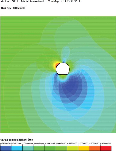
The pattern of displacements around the tunnel excavation, computed on a 500²-point grid, is shown in Figure 4. As shown in the figure, the largest displacements occur around the excavation (orange/red area). As an example, a hardware-accelerated computation to obtain these results required 0.0333 s, while the serial computing time was as long as 4.53 s for the same 500²-point grid.

Figure 4. Displacements around the horseshoe-shaped tunnel for a model size of 5002 points.

The same example model will be used to compare the accelerated implementations of our BEM algorithm to the serial one. The performance of the accelerated implementation will be evaluated as a function of increasing grid sizes from 100² to 1000² in increments of 100² and from 1000² to 1600² in increments of 200². Thus, the results will be computed for 14 grid sizes from 10,000 points to 2.56 million points in total. For each scenario, numbers presented in the subsequent sections are an average of 10 runs, in order to smooth out any performance hits due to external factors, such as Operating System tasks.

2.2. Hardware platforms

The work summarized in this paper considered a set of accelerators: from a single core of a CPU, a multi-core CPU, a desktop GPU, a GPU-based accelerator and an FPGA. When the research was conducted, these accelerators represented a realistic selection of available hardware. The features of each accelerator are summarized in Table 1. Where possible, a reference and a link to the manufacturer’s documentation were given. Since there is a communication between a host and an accelerator to move data back and forth, it was anticipated that the high-memory bandwidth available to the CPU will positively affect (e.g. reduce) the computation time as compared to both the GPUs and FPGA, since the latters were limited by the PCI-E bus’ relatively modest bandwidth.

Table 1. Accelerator specifications

	CPU	Desktop GPU	GPU-Tesla	FPGA
	Intel i7-4770K (Intel, 2015b)	GTX 760 (EVGA, GTX760, 2015)	Tesla K40c (NVIDIA, 2013)	Terasic DE5-Net using Altera Stratix V with 622K logic elements (Terasic Inc., 2015)
Cores	4 (8 threads)	1152	2880	Configurable, see text
Compute units	8	6	15	1
Memory	8 MB L3 cache (32 GB system)	2 GB	12 GB	8 GB
Max. single allocatable memory	512 MB	512 MB	2855 MB	4096 MB
Max. local worksize	1024	1024	1024	64
Frequency	3.5 GHz	1072 MHz	745 MHz (Boost up to 875 MHz)	156.34 MHz (Altera Inc, 2015)
Max. memory bandwidth	25.6 GB/s	192.2 GB/s 15.75 GB/s (PCI-E 3.0)	288 GB/s 15.75 GB/s (PCI-E 3.0)	17 GB/s 15.75 GB/s (PCI-E 3.0)
Thermal design power (TDP)	84 W	170 W	235 W	23.7 W (Altera Inc, 2015)

As seen from Table 1, each accelerator device has unique characteristics when it comes to the number of cores, available memory or power usage. Some of these parameters affect the maximum number of concurrent threads that can be run on an accelerator. In OpenCL, two constants define the number of threads requested to be run; the global worksize and the local worksize. Generally, the global worksize is problem-dependent; for the computation of field quantities, it was taken as the number of field points in a 2D grid, in the range from 100² to 1600², as discussed in Section 2.1. However, the choice for local worksize can significantly affect the efficiency of an accelerated implementation. Each hardware platform has an upper limit on the size of local worksize, as summarized in Table 1. However, the actual number used can influence performance. In order to investigate this, a set of local worksizes were used, from 1 to 64 (as 2ⁱ, i = 0 to 6). For certain model sizes, not all local workgroup sizes were used since the OpenCL specification requires that the global worksize to be evenly divisible by the local worksize (Khronos Group, 2014). Although the accelerators can be used with local worksizes greater than 64, it was found that beyond 64 there is no appreciable gain in performance for any of them. The OpenCL implementation permits to omit the specification for local worksize, thus allowing the OpenCL SDK for select the most appropriate number (Khronos Group, 2014).

2.3. Single core CPU base case

The computation of field quantities using BEM Algorithms 1 and 2 was implemented and used to run the test model. This sequential (or serial, non-OpenCL) implementation will be used as a base-case; all subsequent accelerated implementations will be compared against it. Care was taken that most reasonable optimizations were performed on the code such as loop unrolling, pre-computation of constants outside loops, and multiplication with an inverse, instead of division. Although the length of computation was expected to be the same if the code was run multiple times, the run times shown in Figure 5 are an average of 10 runs. As expected, the correlation for both single- and double-precision computation bears an O(n) relationship as the number of field points is increased. The figure shows computing times for both single- and double-precision runs on the single-core of a CPU (see Section 3.2). The longest run-times for single precision were 37.44 s for the model with 1600² field points, while the longest run-times for double precision were 46.60 s for the model with 1600² field points.

Figure 5. Run times for the serial (non-OpenCL) implementation of Algorithms 1 and 2 for the test model.

2.4. Multi-core CPU accelerated BEM

The multi-core CPU (MCPU) implementation of BEM Algorithms 3 and 4 using OpenCL was executed using all four cores of a CPU. In accordance with the testing parameters set out in Sections 2.1 and 2.2, Figure 6 summarizes the solution times obtained. Time to solution versus the number of field points are plotted for all combinations of local workgroup sizes considered for both single- and double-precision computations. The serial run time is plotted as well, for reference. Figure 6 reveals that the performance curves are stratified for both single and double precision. For small local worksizes (1 through 4), the performance curves are essentially the same. For local worksizes beyond 4, the performance considerably increases; however, the plots still overlap. It is speculated that for the range of 1–4, each core of a CPU gets a single thread scheduled, and above 4 each core gets two threads. The overhead of using OpenCL is evident for small problem sizes (up to about 300² field points), where the serial implementation is actually faster. The ratio of reduction in solution time for local worksizes above 4 to those below 4 is about 3.1 for single precision and 1.96 for double precision. Further discussion on the effect of local worksize is given in Section 3.1, while the difference in single- and double-precision computations in shown in Section 3.2.

Figure 6. Run times for the OpenCL-accelerated MCPU implementation of Algorithms 3 and 4 for the test model (SP – single precision, DP – double precision).

2.5. GPU accelerated BEM

The work presented in the paper considered two GPU-based accelerators: a desktop graphics card (GTX 760) and a purpose-built accelerator (NVIDIA Tesla K40c). Both of these were based on NIVIDIA’s Kepler microarchitecture (NVIDIA, 2013) and represented two common cards available at the time the research was conducted. The OpenCL-based acceleration of the BEM Algorithms 3 and 4 was used in the testing according to the test parameters and conditions set out in Sections 2.1 and 2.2.

2.5.1. Desktop GPU

For the Desktop GPU, Figure 7 summarizes run times for all local worksizes considered, both single and double precision. Considering the operating system-imposed time limit of tying up the GPU for computation (as discussed in Section 2.0), the kernel required multiple invocations. The maximum number of field points that can be computed before triggering the watchdog timer was determined by trial-and-error. Run times reported in Figure 7 incorporate the additional time associated with multiple kernel invocations and extra data transfer and, as discussed before, this amounts to an estimated increase in total computation time by slightly less than 3%. Unlike for the MCPU, the curves for the desktop GPU are distinct for each worksize and the run times decrease with the increasing number of local worksizes. As expected, there is an O(n) relationship between the number of field points and solution times. Although not a surprise for desktop GPUs, the double-precision performance for small local workgroup sizes (up to 8) is actually worse than the serial base-case, owing to the inherent low double-precision capabilities which is a characteristic of the card. A more detailed discussion of this will be given in Section 3.2. The ratio of best-performing run (with 64 for the local worksize) to the single local worksize case was 32.78 for single-precision and 26.83 for double-precision computations.

Figure 7. Run times for the OpenCL-accelerated desktop GPU implementation of Algorithms 3 and 4 for the test model (SP – single precision, DP-double precision).

2.5.2. Tesla GPU

Although based on the same microarchitecture, the Tesla GPU card was designed for high-end scientific computation. It is not affected by the watchdog timer timeout as the Desktop GPU. The same set of local worksizes were used for executing the example problem and the run times are plotted in Figure 8. Similar to the Desktop GPU, for each increase in local worksize, the solution time decreased while maintaining an O(n) relationship. Both the single-precision and double-precision results are better (lower solution time) than the serial implementation. However, the cost of OpenCL setup and data transfer overhead is observable for small problem sizes. The double-precision performance of the Tesla GPU is considerably better than the Desktop GPU. For small local worksizes, it is marginally better than the serial implementation, further underlining that GPUs were meant to run many concurrent threads of execution to achieve good performance. The ratio of best-performing run (with the local worksize of 64) to a single local worksize case was 32.69 for single-precision and 26.90 for double-precision computations, almost identical to the Desktop GPU. Relative speedups will be discussed in detail in Section 3.0.

Figure 8. Run times for the OpenCL-accelerated Tesla GPU implementation of Algorithms 3 and 4 for the test model (SP – single precision, DP – double precision).

2.6. FPGA accelerated BEM

Due to its nature, the FPGA hardware accelerator is different than an MCPU or a GPU. The FPGA is mainly defined by its number of available gates or logic elements, which can accommodate a hardware description of the algorithms to be run. The hardware synthesis of BEM Algorithm 4 can be influenced by the number of cores requested, which is limited by the number of logic elements. Other factors, such as the available memory can influence the design as well. Depending on the size of an algorithm (e.g. number of instructions, type of instruction, quantity and type of data to be operated on, etc.) the FPGA might not have a sufficient number of gates, as was found for the case of double-precision algorithm. Thus, only single-precision results are available in this paper. It is expected, given a larger-size FPGA, that the double-precision implementation can be achieved as well. The BEM Algorithm 4 was synthesized using Altera’s Quartus II suite and the example problem was run according to test parameters and conditions set out in Sections 2.1 and 2.2. Run times for the range of field points and local worksizes are shown in Figure 9. The solution times generally decrease with an increasing local worksize, while more-or-less maintaining an O(n) relationship.

Figure 9. Run times for the OpenCL-accelerated FPGA implementation of Algorithms 3 and 4 for the test model (SP – single precision).

For local worksizes of 1 and 2, the FPGA’s performance is lower than the base serial implementation; a worksize of 1 takes over twice as long as the serial implementation. For worksizes greater than 2, the performance gradually improves, but there is little difference between 32 and 64, signalling an upper limit of performance gains. The ratio of best-performing run (with the local worksize of 64) to the single local worksize was 30.96 for single-precision.

3. Performance comparisons

Although results presented in Sections 2.4 through 2.6 show solution times for an example problem for each accelerator along with the unaccelerated, serial computation times, it is hard to evaluate relative performance gains offered by each accelerator. Run times can help to compare the effectiveness of an algorithm, its implementation and the benefits offered by a specific hardware platform. More commonly though, relative speedup, as defined by Pacheco (Pacheco, 1997), can be used to compare different implementations. However, in our energy-conscious world, a growing emphasis is placed on the actual energy used in performing a task. Thus, for our computations, an additional metric is introduced; the speedup-per-watt (Bischof, 2008). While this section focuses on the comparison of relative speedups, the speedup-per-watt will be discussed in Section 3.3.

The purpose of any ranking based on relative speedup is to guide our choice when it comes to acquiring new hardware either to replace or supplement what is currently available. Therefore, it is a logical choice to base our comparisons on an un-accelerated, serial implementation running on a single core of a CPU before hardware-accelerated versions are implemented. However, the majority of currently available CPUs have more than one core. Therefore, at no extra investment, we have at our disposal a hardware accelerator. In this case, it is sensible to modify our performance metric (the relative speedup) to compare other accelerators to the multi-core CPU (MCPU). This growing sentiment of what serves as a good base case was voiced in literature as well (Lee et al., 2010).

Figure 10 summarizes relative speedups achieved by various accelerators using a single core, serial implementation as a base case. Both single and double-precision results are plotted and both sets of curves exhibit the same characteristics. Thus, without loss of generality, this section considers the single-precision results only, while Section 3.2 will examine the relative performance based on single or double-precision computations. For each accelerator discussed in Sections 2.4–2.6, the best-performing case was selected (the ones with the largest local worksize, as mentioned before). All speedup curves display a similar trend; there is a relatively sharp rise in speedup for small problem sizes (as measured by the number of field points), which levels off as the problem size increases. The MCPU offers speedups from below one for small problem sizes (100² to 400²) to as high as 5 for larger problems (1400² and greater). Even though the theoretical maximum would be 8 if all cores are fully utilized, in practice it is almost unattainable. Thus, the relative speedup of 5 for a MCPU is a reasonable one, considering that no additional hardware was required to attain it. For the GPU-based accelerators considered, the Tesla GPU achieves the highest speedups, followed by the Desktop GPU. For larger problem sizes (1400² and greater) the speedup reached above 134 with a slight drop in speedup as the problem size further increased. The Desktop GPU shows an almost identical trend, albeit with a maximum speedup of about 110 for larger problem sizes. The last hardware accelerator considered, the FPGA, unfortunately shows much more modest performance gains; it only achieves a speedup of about 12.5 for larger problems, positioning it above the MCPU in performance. It appears that GPU-based accelerators offer the greatest achievable speedups among the hardware considered, based on the comparison with the serial implementation.

Figure 10. Speedups achieved by various implementations as compared to the serial case.

If the relative speedup comparison is based on the MCPU as a base case, Figure 11 shows that both GPU-based accelerators reach a relative speedup of about 20 (maximum of 22 for the Tesla GPU and 18.3 for the Desktop GPU). The GPUs’ relative speedup seems to steadily drop after reaching their peak. This is attributable to the combined effect of drop in GPU performance and increase in the MCPU performance for large problem sizes, as already discussed in relation to Figure 10. The FPGA reaches a peak relative speedup of about 2 and drops slightly to 1.7 towards the right of the figure. As expected, if the MCPU is used as the base case, the relative speedups are not nearly as high as for the serial case. Yet, the GPU-based accelerators achieve a speedup as high as 22 over the MCPU.

Figure 11. Speedups achieved by various implementations as compared to the MCPU case.

3.1. Effect of local workgroup size

It is evident from Figure 6 through 9 that the local worksize plays an important role in the resulting computation time. Since all accelerators are based on a principle that multiple concurrent threads of execution are running, if only a single thread is run, the performance will be far from optimum. As an upper limit, the maximum number of concurrent threads in a workgroup is summarized Table 1. Ideally, performance should increase with an increasing number of concurrent threads in a workgroup. However, in that case more threads are accessing common constants and variables in the shared memory, perhaps impacting performance. Another way to look at the data summarized in Figure 6 through 9 is to plot the solution time vs. local worksize for each problem size. For the sake of brevity these plots are only included in this paper for the MCPU and Tesla GPU (as shown in Figures 12 and 13), for the single-precision computation only, while similar trends were observed for the Desktop GPU and FPGA as well. The double-precision results exhibited a very similar trend also. For the MCPU, the local worksize between 1 and 4 has little effect on performance. For a worksize of eight, there is a sharp increase in performance (drop in solution time), and beyond which, with increasing worksize, there is little or no further improvement. The worksizes considered in this paper, as presented in Section 2.2, were all integer powers of two. But for example, if worksize of 10 was used, the performance suddenly drops by as much as 40% (if compared to a worksize of 8), as seen on Figure 12. This re-iterates that, although tempting to use local worksizes that we are more accustomed to (powers of 10), there could be a performance drop. However, by using powers of two for local worksize either the global worksize has to be adjusted or some combinations of local and global worksizes are not possible any more. Figure 13 summarizes performance for the Tesla GPU; in contrast to Figure 12, increasing the local worksize starting with one translates into increased performance. Unlike the MCPU, for the Tesla GPU there is no performance drop if non-power of two local worksizes were used; Figure 13 contains data for 10 and 50 as the local worksize, without any performance penalty. Similar to the MCPU, worksizes beyond 50 or 64 offer no appreciable speed increase. Although not shown, the same conclusions can be drawn for both the Desktop GPU and FPGA.

Figure 12. Solution times as a function of local worksize – MCPU.

Figure 13. Solution times as a function of local worksize – Tesla GPU.

3.2. Single precision vs. double precision – speedup and accuracy

Accuracy is of importance for numerical computation in engineering and science. Many numerical models and methods, like solution of a system of equations, are sensitive to round-off errors or the number of significant digits in input parameters. Thus, most of these methods generally employ double-precision computation. Even though the accuracy in computation is important, one has to consider the quality of input parameters. For example, in geomechanics, most input parameters, like rock mass properties, are seldom know within 20–30% of their true mean (Starfield & Cundall, 1988), presenting an opportunity for accepting “less-than-accurate” computation. To investigate the potential loss of accuracy and perhaps speed gains, Algorithms 1–4 were modified to use double-precision constants and variables. Also, appropriate arithmetic functions (e.g. going from fabsf() to fabs()) were used to avoid unnecessary casts resulting in speed reduction. All test cases were re-run using double precision for both the serial algorithm and the hardware-accelerated ones, where double-precision computation was possible.

Figure 5 shows that for the serial (single-core) case there is an approximately 20% performance drop if double-precision computation is used for larger problems, while the greatest difference in solution, measured using $L_{\mathrm{\infty }}$norm, was 0.00093% across all modelled cases (grid points from 100² to 1600²) for the computed displacements. While Figures 6 through 9 show the single- and double-precision performance for each accelerator, Figure 10 contains the composite results expressed as relative speedup. Double-precision computations on the OpenCL-accelerated MCPU, for larger problem sizes, take on average 9% longer than in single-precision, while the difference in solution across all modelled cases, using a $L_{\mathrm{\infty }}$norm, was 0.00125%. The mere 9% increase in computation time is not surprising since the MCPU is a general-purpose chip, with good floating-point performance for both single and double precision. Actually, compared to the serial (single-core) case, where the cost of double precision was 20% extra time, the performance of the MCPU was very good. For the GPU-based accelerators, it was found that the double-precision performance of the Desktop GPU was on average 26 times slower than its single-precision computation. In interpreting this low performance, one has to consider that most computer graphics operations on a GPU are optimized for single-precision. Literature reports that the double-precision performance of Kepler microarchitecture desktop GPUs is 1/24 of their single-precision performance (Arrayfire, 2015), which confirms our findings. The difference in solution of displacements across all modelled cases using $L_{\mathrm{\infty }}$norm was 0.00147% on the Desktop GPU. However, the same source reports that the Kepler microarchitecture-based Tesla GPU has a substantially better double-precision floating point performance (1/3 of single-precision). Our results indicate that double-precision computations on the Tesla GPU were on average 3.8 times slower than single-precision ones, which is similar to what literature reports. For this platform, the maximum difference in results, as measured by a $L_{\mathrm{\infty }}$norm, was 0.00132% between the single and double-precision results. As mentioned before, the FPGA-based accelerator was only able to synthesize the single-precision algorithms; thus, we cannot compare the performance.

In summary, most hardware accelerators are capable of carrying out computations in both single- and double-precision without considerable degradation in accuracy. However, based on the design philosophy behind each accelerator, its double-precision performance can vary significantly. Even though the Tesla GPU’s double-precision performance is about one-quarter of its single-precision one, it is still almost 40 times faster than the serial (single core) of a CPU. If the basis of comparison is the MCPU, the Tesla GPU is on average five times faster than the MCPU for double-precision calculations, as seen in Figure 11. Unfortunately, the Desktop GPU’s double-precision performance is on par with the MCPU; thus, it does not offer performance improvement in double-precision computations.

3.3. Speedup-per-watt

Although most accelerators are preferred in order to expedite the completion of a computing task, in the current energy-conscious climate, the use of energy is becoming important. Table 1 summarizes the power consumption of hardware accelerators. However, these are individual components only. Many of them cannot function alone; a computer system requires power for the CPU, motherboard, memory, GPU and other accessories. Thus, to measure the minimum power required to run the system, different scenarios were devised based on what accelerator was used, as summarized in Table 2. For each scenario, the largest model (with 1600² grid points) was run for 10 times. For each run, the power was sampled at 1-ms intervals using an in-line energy usage monitor. The power consumptions in Table 2 are an average within each run and also averaged over the 10 runs.

Table 2. Scenarios for power consumption testing

Scenario	Active components	Average power consumption (W)
Single-core CPU	CPU, Motherboard, RAM^a	53.7
Multi-core CPU	CPU, Motherboard, RAM^a	72.1
Desktop GPU	CPU, Motherboard, RAM plus GPU	135.6
Tesla GPU	CPU, Motherboard, RAM plus Tesla GPU^a	178.5
FPGA	CPU, Motherboard, RAM plus FPGA^a	78.6

Note: ^aThe system was run headless, accessed remotely via VNC.

Interestingly, the actual power consumption of the system is somewhat different than what the sum of active components suggests. For all cases, the system power usages were lower than what the components indicate. For example, Table 1 indicates that the CPU’s design power was 84W, while the single-core scenario consumed on average 53.7W and the multi-core one needed 72.1W, both of which were below the values indicated in Table 1, considering that the motherboard and memory consumed some energy as well. Similarly, for the Tesla GPU, Table 1 lists 235W and the system power consumption (including CPU, memory, etc.) required 178.5W in total. Only for the FPGA the system power consumption was in line with Table 1, where 23.7 W was predicted for the FPGA. Adding this on top of the single-core CPU scenario resulted in approximately the measured power usage.

Having determined the actual power consumption of the system for each scenario, the data in Figure 10 can be updated by dividing relative speedup by the power usage, expressed as a speedup-per-watt metric. This new metric is shown in Figure 14. For single-precision computations, the lower relative power consumption of the Desktop GPU (in comparison to the Tesla GPU) results in the best performance in contrast to Figure 10. The FPGA ranks third, slightly above the MCPU; thus, the FPGA presents a viable alternative to CPUs where low-power acceleration is required. However, for double precision, the Tesla GPU still achieves the highest performance, followed by the MCPU and Desktop GPU, reversing the ranking for the last two. In closing, overall the Tesla GPU appears to be the highest performer even when the power consumption is considered.

Figure 14. Speedup-per-watt achieved by various implementations as compared to the serial case.

4. Conclusions

Computation in engineering and science can be challenging. Both the formulation of a mathematical model and its evaluation in a timely manner can be detrimental in the model’s widespread use. A method such as the BEM, often used in geomechanics, was selected as an example of a numerical method, which can be benefitted from acceleration. The computation of field quantities, such as stresses and displacements, in a BEM model can be performed in parallel. This paper considered the acceleration of computation on a wide variety of hardware accelerators from multiple cores of a CPU, through the use of GPUs, and finally considering FPGAs. Each hardware accelerator presented different challenges because some of them were designed for parallel execution using a large number of concurrent threads (GPUs), while others were designed to run a relatively small set of simultaneous threads (e.g. the number of cores on a multi-core CPU). FPGAs, relative newcomers amongst the OpenCL-based accelerators, were considered in this study for their low power consumption, representing an energy-conscious alternative. Upon performing computation on the hardware accelerators and evaluating their relative performance using various metrics, such as relative speedup, the following conclusions can be drawn:

• If maximum performance is needed, currently Tesla GPUs present the best option. Even though their power requirements are the highest, their performance ranks highest in both single and double-precision computation.

• While for no additional investment, the multi-core CPU OpenCL version of the BEM algorithm offers a modest (five-fold) speedup.

• Although Desktop GPUs were not meant for double-precision computation, if a single-precision formulation of a numerical model can be used, their performance is very high.

• Even though FPGAs offer an energy conscious alternative, currently their comparatively low speedup and long kernel compilation times could detract from their potential to be used as accelerators, at least for this class of BEM computation.

• Intentionally, the cost of hardware and software needed was not included in the study; however, if cost is a consideration and single-precision computation is adequate, commonly available Desktop GPUs offer the best value.

Additional information

Funding

This work was supported by the Concordia ENCS Faculty Graduate Support program (GSSP) and the Natural Sciences and Engineering Research Council of Canada’s (NSERC) Discovery Grant program,Concordia University – NSERC Govt. Canada [grant number N01088].

Notes on contributors

Junjie Gu

Junjie Gu completed her Master of Applied Science graduate degree in 2016 under the supervision of Dr Zsaki. Her research interests are computer applications in geomechanics and parallel processing.

Attila Michael Zsaki

Attila Michael Zsaki is an associate professor in the Department of Building, Civil and Environmental Engineering. He obtained his BE degree from Ryerson University and his MSc and PhD degrees in civil engineering from the University of Toronto. Dr Zsaki’s research is focused on modelling and computational aspects of geosciences with particular interest in multiphysics modelling of continuum and discontinuum. His other areas of interest are scientific computing, parallel computing, computer graphics and mesh generation. In addition to academia, Dr Zsaki has worked in the industry as software developer and consultant for a geomechanics analysis software company, and lately on high-performance scientific computing applications for modelling continuum behaviour. His interests are performance optimization and parallel computing on scalable, shared-memory multiprocessor systems, graphics processing units (GPU) and FPGAs.

References

- Altera Inc . (2014). Altera quartus II . Retrieved from http://dl.altera.com/?edition=pro
- Altera Inc . (2015). Altera quartus II – PowerPlay power analyzer tool . Retrieved from http://dl.altera.com/?edition=pro
- Arrayfire . (2015). Explaining FP64 performance on GPUs . Retrieved from http://arrayfire.com/explaining-fp64-performance-on-gpus
- Bischof, C. (2008). Parallel computing: Architectures, algorithms, and applications . Amsterdam, The Netherlands: IOS Press.
- Brebbia, C. A. , & Partridge, P. W. (1992). Boundary elements in fluid dynamics . Netherlands: Springer.
- Cooper, C. D. , Bardhan, J. P. , & Barba, L. A. (2014). A biomolecular electrostatics solver using Python, GPUs and boundary elements that can handle solvent-filled cavities and Stern layers. Computer Physics Communications , 185(3), 720–729. doi:10.1016/j.cpc.2013.10.028
- Crouch, S. L. , Starfield, A. M. , & Rizzo, F. (1983). Boundary element methods in solid mechanics. Journal of Applied Mechanics , 50, 704. doi:10.1115/1.3167130
- EVGA, GTX760 . (2015). Retrieved from http://www.evga.com/Products/Specs/GPU.aspx?pn=D34D9B88-00D7-4F24-A92D-76ECD7BB6346
- Gu, J. (2015). GPU-accelerated boundary element method for stress analysis of underground excavations ( Master’s Thesis). Dept. of Building, Civil and Environmental Engineering, Concordia University, Montreal, QC, Canada
- Haase, G. , Schanz, M. , & Vafai, S. (2012). Computing boundary element method’s matrices on GPU, in large-scale scientific computing. In I. Lirkov , S. Margenov , & J. Waśniewski (Eds.), 8th international conference, LSSC 2011, Sozopol, Bulgaria, June 6–10, 2011, Revised Selected Papers (pp. 343–350). Berlin, Heidelberg: Springer Berlin Heidelberg.
- Intel . (2015a). OpenCL SDK . Retrieved from https://software.intel.com/en-us/intel-opencl
- Intel . (2015b). Intel® Core™ i7-4770K Processor . Retrieved from http://ark.intel.com/products/75123/Intel-Core-i7-4770K-Processor-8M-Cache-up-to-3_90-GHz
- Khronos Group . (2014). OpenCL . Retrieved from https://www.khronos.org/opencl/
- Kythe, P. K. (1995). An introduction to boundary element methods . Boca Raton, FL: CRC press.
- Lee, V. W. , Kim, C. , Chhugani, J. , Deisher, M. , Kim, D. , Nguyen, A. D. , … Singhal, R. , 2010, Debunking the 100X GPU vs. CPU myth: an evaluation of throughput computing on CPU and GPU . Proceedings of the 37th annual international symposium on Computer architecture (pp. 451–460). ACM New York, NY, USA. doi:10.1177/1753193410364178
- Microsoft . (2012). Visual studio ultimate . Retrieved from https://www.microsoft.com/en-ca/download/details.aspx?id=30682
- Molavi Tabrizi, A. , Goossens, S. , Mehdizadeh Rahimi, A. , Cooper, C. D. , Knepley, M. G. , & Bardhan, J. P. (2017). Extending the solvation-layer interface condition continuum electrostatic model to a linearized Poisson-Boltzmann solvent. Journal of Chemical Theory and Computation , 13(6), 2897–2914. doi:10.1021/acs.jctc.6b00832
- NVIDIA . (2013). Tesla K40 GPU Active Accelerator . Retrieved from http://www.nvidia.com/content/PDF/kepler/Tesla-K40-Active-Board-Spec-BD-06949-001_v03.pdf
- NVIDIA . (2014). CUDA Toolkit . Retrieved from http://docs.nvidia.com/cuda
- Pacheco, P. S. (1997). Parallel programming with MPI . San Francisco, USA: Morgan Kaufmann.
- Poljak, D. , & Brebbia, C. A. (2005). Boundary element methods for electrical engineers (Advances in electrical engineering and electromagnetics) . Ashurst, Southampton: WIT Press.
- Starfield, A. M. , & Cundall, P. A. (1988). Towards a methodology for rock mechanics modelling. International Journal of Rock Mechanics and Mining Sciences and Geomechanics Abstracts , 25(3), 99–106. doi:10.1016/0148-9062(88)92292-9
- Terasic Inc. (2015). DE5-net user manual . Retrieved from http://www.terasic.com.tw/attachment/archive/526/DE5NET_OpenCL.pdf
- Torky, A. A. , & Rashed, Y. F. (2017). GPU acceleration of the boundary element method for shear-deformable bending of plates. Engineering Analysis with Boundary Elements , 74, 34–48. doi:10.1016/j.enganabound.2016.10.006
- Zsaki, A. M. (2011, October 2–6) GPU-accelerated stress analysis in geomechanics. 64th Canadian Geotechnical Conference and 14th Pan-American Conference on Soil Mechanics and Geotechnical Engineering, Toronto, Canada