Uncertainty assessment of onset sand prediction model for reservoir applications

Abstract

Modeling physical systems in engineering always comes with uncertainties in terms of the model’s input parameters. These uncertainties are also present in modeling the onset of sand production, even though considerable effort may be required in incorporating uncertainties into the process of modeling, because getting it right will definitely provide important knowledge about the input parameters for predicting the onset of sanding which provides useful hints that inform apt decision-making for sand control. In this study, a Monte Carlo simulation of some parametric input variables alongside the incorporation of the Hoek–Brown material constants was investigated using a predictive model for sand production anchored on Hoek–Brown failure criterion, so as to rank some key input uncertainties in order of the effect their magnitudinal disparities on the model output. The key inputs in the model are reservoir pressure, rock strength (uniaxial compressive strength, UCS), minimum horizontal stress, Poisson’s ratio and Hoek–Brown material constants M and S.

Different diagnostic Tornado and spider plots were generated and interpreted for two wells and it was observed that the predicted well pressure is most sensitive to rock strength and generally has an inverse relationship with the rock strength. The parametric study on Hoek–Brown material constants shows that higher values of M and S correspond to lower minimum well pressure at which sanding is expected. The model is a useful tool for a quick assessment of the onset of sanding in reservoir rocks and can also be used to evaluate the effect of different rock mechanical properties.

Keywords:

• sanding
• failure criterion
• uncertainty assessment
• Hoek–Brown

PUBLIC INTEREST STATEMENT

70 per cent of oil and gas production around the world today comes from unconsolidated sandstone reservoirs. These reservoir rocks are prone to sand production at some stage during the production life of the well. Predicting when the well will be a sand producer and what volumeof sand will be produced alongside production fluid has been the major concern for oil and gas operators. Therefore, numerous predictive tools have been developed over the last decades but with different degrees of uncertainties in their input parameters which could impact the predictive accuracy. Hence, this work presents the results of uncertainty assessment of sand prediction model for reservoir applications. In this study, a Monte Carlo simulation of some parametric input variables alongside the incorporation of the Hoek–Brown material constants was investigated using a predictive model for sand production, anchored on Hoek–Brown failure criterion. The model is useful for quick assessment of sanding in reservoir rocks.

1. Introduction

Assessment of sanding tendency during development and completion stages of oil and gas wells is fast becoming popular and common practice amongst oil and gas operators (Asadi, Pham. Le Minh & Butt, 2015). As environmental conditions such as nature of oil formation zones become challenging, drilling and completing a well becomes more expensive and with real-time sand production predictive tools, change in stability of load-bearing sands can be tracked and also the minimum well pressure at/below which sand production is to be expected can be predicted. With these predictive tools, making real-time economically wise decisions becomes easy (Vahidoddin, Mahdi, & Mehranpour, 2012). Sanding is a two-stage phenomenon which includes the first stage of reservoir rock formation failure which is immediately followed by transport of formation materials by the flowing fluid. The first stage is stress-induced which subsequently enhances the flow velocity for onward transportation of the detached sands (Venkitaraman, Behrmann, & Chow, 2000). To comprehensively understand the subject of sand production, several factors have to be considered:

• Drilling operation practices

• Production parameters

• Rock mechanical properties and

• Rock mineralogy (composition)

However, change in stress field around the wellbore which has a direct impact on rock strength has been reported to have the most significant effect on sand production in oil wells (Isehunwa & Olanrewaju, 2010; Isehunwa, Ogunkunle, Onwuegbu, & Akinsete, 2017). In order to manage reservoirs and wells that are sand producers to deliver maximum production rate at minimal operating cost, an integrated approach to sand management is required. According to Oyeneyin (2005), the conventional stepwise approach to sand management includes

• Sand production risk assessment through a predictive tool

• Selection of appropriate sand control options

• Downhole sand grain and produced volumemonitoring

• Topside management

Of all the stages, the key to sand management and control is being able to effectively predict when and if sanding will occur and this is usually done before the well is completed. However, it is important to note that modeling physical systems in engineering often come with some level of uncertainties in terms of the model’s input parameters. These uncertainties are equally present in the input parameters for any sand predictive tool. Knowing these uncertainties can impact on the accuracy of sand predictive tools which in turn helps in making apt sand control decision. Uncertainty assessment (sensitivity analysis) helps in ranking key input uncertainties in order of magnitude of their effect on the model output. Numerous recently published work on mechanical modeling of rock failure shows the influence of various field and operational parameters on continuous and transient sanding (e.g Asadi et al. 2017; Araujo et al., 2014; Asadi, Khaksar, Ring, Saric, & Yin Yin, 2016; Gui, Khaksar, Zee, & Cadogan, 2016; Lamorde, Somerville, & Hamilton, 2014; Morita, Whitfill, Fedde, & Levik, 1989; Zhang et al., 2017). Most of these works successfully modeled sand production onset, but were all anchored on Mohr failure criterion which assumed rock mass quality to be 100 per cent intact and could not account for different levels of disturbance in terms of rock strength. Therefore, the analytical model used in uncertainty assessment in this study is strongly anchored of Hoek–Brown failure criterion that is applicable for different rock mass conditions.

This study presents the results of uncertainty assessment of some input variables for a sand predictive tool whose origin spans from application of failure criterion by Hoek, Carranza-Toress, and Corkum (2002). The model is a very reliable prediction tool that can be used before a well is completed and solely relies on log information obtained while drilling.

2. Model development

The key to developing a sand predictive tool is identifying and developing stress equations around the perforation cavity and appropriating the right failure criterion (Almisned & Abdulaziz, 1995).

The approach in this model will be based on the listed assumptions as discussed in Almisned and Abdulaziz (1995):

• The horizontal stress is isotropic at far away from the well

• The rock is a homogenous, unconsolidated or poorly consolidated sandstone

• The formation is in a geologically relaxed environment and there is no active tectonic regime within the formation.

• Shear failure corresponds to the initiation of sand production, i.e., drag forces are ignored.

• Stress controlled failure process around the perforation cavity is dominated by cohesion loss and not by frictional strength loss.

• The wellbore/perforation tunnel-formation structure is axisymmetric.

• Formation rock failure can be described by modified Hoek–Brown failure criterion.

According to Fjaer, Holt, Horsud, Raaen, and Risnes (1992) the stress at the borehole can expressed as follows:

(1) ${{\sigma }_r}^{\prime }=\left(1-\alpha \right)P_{wf\left(t\right)}$(1)

(2) ${{\sigma }_{\theta }}^{\prime }=2{\sigma }_{h\left(t\right)}-\alpha \frac{1-2\nu }{1-\nu }{\bar{P}}_{\left(t\right)}-\left(1+\alpha \frac{\nu }{1-\nu }\right)P_{wf\left(t\right)}$(2)

The Hoek–Brown failure criterion in terms of borehole stress is then given as follows:

(3) ${{\sigma }_{\theta }}^{\prime }={{\sigma }_r}^{\prime }][+C_o{\left(M\frac{{{\sigma }_r}^{\prime }}{C_o}+s\right)}^{0.5}$(3)

Hoek–Brown material constant M and S is as follows (Hoek et al. 2002):

(4) $M=m_{i}exp\left(\frac{GSI-100}{24-14D}\right)$(4)

(5) $S=exp\left(\frac{GSI-100}{9-3D}\right)$(5)

It is assumed that the effective tangential stress is largest at the borehole wall; therefore, stability occurs when (2) is equal to (3) as follows:

(6) $2{{\sigma }_h}_{\left(t\right)}-\alpha \frac{1-2\nu }{1-\nu }{\bar{P}}_{\left(t\right)}-\left(1+\alpha \frac{\upsilon }{1-\upsilon }\right){P_{wf}}_{\left(t\right)}=\left(1-\alpha \right){P_{wf}}_{\left(t\right)}+C_o{\left[M\frac{\left(1-\alpha \right)P_{wf}}{C_o}+S\right]}^{0.5}$(6)

The resulting equation from (6) yields a quadratic equation on squaring both sides of the equation and is solved using the general solution to quadratic equation as follows:

If $n=\frac{1-2\nu }{1-\nu }$

${\left(2-\propto n\right)}^2{P_{wf}}^2-P_{wf}\left[M{C}_o\left(1-\propto \right)-2\left(2-\propto n\right)\left(\propto n\bar{P}-2{\sigma }_h\right)\right]+{\left(\propto n\bar{P}-2{\sigma }_h\right)}^2-S{C_o}^2=0$

(7) $x=-\frac{b\pm \sqrt{b^2-4ac}}{2a}$(7)

$a={\left(2-\propto n\right)}^2$

$b=\left[M{C}_o\left(1-\propto \right)-2\left(2-\propto n\right)\left(\propto n\bar{P}-2{\sigma }_h\right)\right]$

$c={\left(\propto n\bar{P}-2{\sigma }_h\right)}^2-S{C_o}^2$

Let $R=\left(2-\propto n\right)Y=\left(\propto n\bar{P}-2{\sigma }_h\right)U=\left(1-\propto \right)$

Then, we have

$a=Rb=M{C}_{o}U-2RYC=Y^2-S{C_o}^2$

Therefore, $P_{wf}$ is given as follows:

(8) $P_{wf}=\frac{-\left(M{C}_{o}U-2RY\right)\pm \sqrt{M{C}_{o}U-2R{Y}^2-4R^2\left(Y^2-S{C_o}^2\right)}}{2R^2}$(8)

The final equation (i.e., Eq. 8) is the minimum well pressure at/below which sanding is to be expected. The key input parameters are the uniaxial compressive strength (UCS), designated as rock strength “C_o” in this study, reservoir pressure, minimum horizontal stress, Poisson’s ratio and Hoek–Brown material constant M and S, which can be estimated from (4) and (5) together with geological strength index as obtained from the chart of Marinos, Marinos, and Hoek (2005); typical values of M and S are presented in Table 1 for different rock conditions especially in situations where it is extremely difficult to identify the correct condition of the reservoir rock. The constant M is synonymous to the instantaneous friction angle of intact rocks for Mohr envelope and analogous to reservoir rocks frictional strength. It is the reduced value of m _i in the original Hoek–Brown failure criterion (1980). Material constant M was introduced to the Hoek et al. (2002) to account for the strength reducing effects of rock mass conditions, while S is a constant that varies as a function of how fractured the rock is from a maximum value of 1 for intact rock to zero for heavily fractured rock where the tensile strength is insignificant or negligible.

Table 1. Hoek–Brown material constants for different rock mass conditions

Rocks	Carbonates rocks	Shale	Sandstone	Fine-grained igneous rocks	Coarse-grained igneous rocks
Intact rocks	M = 6 S = 1	M = 8 S = 1	M = 11 S = 1	M = 16 S = 1	M = 18 S = 1
Undisturbed Rocks	M = 3 S = 0.189	M = 4.39 S = 0.189	M = 5.59 S = 0.189	M = 7 S = 0.189	M = 12.56 S = 0.189
moderately Weathered Rocks	M = 7 −1.6. S = 1	M = 1 −0.923. S = 1	M = 1.6–3.02 S = 1	M = 1.6–4.81 S = 1	M = 3.3–6.51 S = 1
heavily weathered rocks	M = 0.03 S = 0.00002	M = 0.043 S = 0.00002	M = 0.65 S = 0.00002	M = 0.0746 S = 0.00002	M = 0.109 S = 0.00002

3. Geologic setting of the study area

The wells used in this study are located in the Niger Delta oil fields situated in the Gulf of Guinea, that extended throughout the Niger Delta Province according to Klett, Ahlbrandt, Schmoker, and Dolton (1997), as cited by Tuttle, Charpentier, and Brownfield (1999). The depobelts formed are results of progradation of the deltaic sediments from Eocene to Present representing the most active part of the delta at different stages of its development (Doust and Omatsola, 1990 as cited in Tuttle et al., 1999). These depo-belts represents one of the world largest regressive deltas with an estimated area of some 300,000 km² (Kulke, 1995 as cited in Tuttle et al., 1999), a sediment volumeof 500,000 km³, and a sediment thickness of over 10 km in the basin depocentre (Kaplam, Lusser, and Norton, 1994, 1995 as cited in Tuttle et al., 1999). One recognized petroleum system has been reported in the Niger Delta Province (Kulke, 1995; Ekweozor, and Daukoru, 1994 as cited in Tuttle et al., 1999), which is the Tertiary Niger Delta (Akata—Agbada) Petroleum System, the lithostratigraphic units in the basin consist of Akata Formation at the base which is the oldest, (strictly shale lithology and considered to be the source rock) Paleocene to Holocene in age, this was ovelained by the para-sequence of sandstone and shale beds of the Agbada Formation, considered to be the reservoir rock, Tertiary to recent in age.

The extreme extent of the Tertiary Niger Delta petroleum system corresponds with the boundaries of the province while the lowest extent of the system corresponds to the areal extent of fields and also known to contain commercial quantity of hydrocarbon (i.e., cumulative production plus proved reserves as at 2017) of about 37 billion barrels of oil (BBO) and 192 trillion cubic feet of gas (TCFG) (World data Atlas, 2017). Most of the oil production comes from onshore fields or continental shelf with water depth of less than 200 m, and are hosted primarily in large but relatively simple structures but in recent times, oil productions has moved into deep waters. The trapping mechanism in the petroleum system has been identified to be both structural and stratigraphic traps (i.e., interbedded shale, growth faults and rollover anticlines) formed as a result of instability of the over-pressured and under-compacting Akata shale.

4. Results

Tables 2 and 3 present the production statistics for the two wells used in this study including the sand production profile in terms of sand volumeproduced at different operating conditions, they are generally recorded during routine production test. Tables 4 and 5 show the reservoir rock mechanical properties for the wells. The details of the ideologies and correlations used in estimating these properties are presented in the work of Khaksar et al. (2009). The output results corresponding to each wells were only presented here. The reservoirs penetrated for the wells were found between 7250–7497 ft and 7100–7615 ft for wells X1 and X2, respectively. Data presented in Tables 3 and 4 together with Eq. 8 were used to assess the sand production potential of the wells in terms of minimum well pressure at sanding and the results compared favorably with the field well pressures imposed on the wells (2000 psi for well X1 and 2300 psi for well X2). The results of the comparisons are presented in Figures 1 and 2, while parametric study of the model’s response to changes in values of Hoek–Brown material constants is also evaluated with respect to field imposed well pressures. The analysis is presented in the next section.

Table 2. Average sand production for well X1

Sand (PPTB)	Oil (bbl/m)	Water (bbl/m)	Water-cut (%)	Gas (Msc/m)	GLR (Scf/bbl)
2	54,279	31	0	11,063	204
0	21,540	8	0	9525	442
1	13,506	5814	30	5550	287
1	3646	1497	29	1024	199
2	39,280	16,440	30	7541	135
2	38,743	7399	16	6933	150
2	23,049	4228	15	4778	175

Table 3. Average sand production data for well X2

Sand (PPTB)	Oil (bbl/m)	Water (bbl/m)	Water cut (%)	Gas (Mscf/m)	GLR (scf/bbl)
40	13,081	36,322	74	5919	120
34	17,137	14,032	45	82,393	2643
33	15,323	11,686	43	2899	107
33	14,850	10,520	41	19,075	752
33	19,788	14,790	43	14,550	421
33	18,150	13,607	43	15,624	492
33	18,615	13,327	42	5813	182

Table 4. Rock mechanical properties for well X1

Depth (ft)	Overburden pressure (psi/ft)	Pore pressure (psi/ft)	Min horizontal Stress (psi/ft)	Max horizontal stress (psi/ft)	Poisson’s ratio	Rock strength (psi)
5843	0.821	0.471	0.6136	0.6636	0.28	3548
5980	0.832	0.422	0.6297	0.6797	0.28	3478
6060	0.84	0.426	0.6431	0.6931	0.28	3556
7201	0.849	0.391	0.6811	0.7311	0.28	4096
7271	0.861	0.402	0.7245	0.7745	0.28	4222
7345	0.882	0.397	0.7431	0.7931	0.28	4303
7484	0.902	0.392	0.7461	0.7961	0.28	4418
7575	0.962	0.369	0.8125	0.8625	0.28	4542
7638	0.981	0.383	0.8411	0.8911	0.28	4703

Table 5. Rock mechanical properties for well X2

Depth (ft)	Overburden pressure (psi/ft)	Pore pressure (psi/ft)	Min horizontal stress (psi/ft)	Max horizontal stress (psi/ft)	Poisson’s ratio	Rock strength (psi)
5694	0.8211	0.43	0.715	0.765	0.28	3314
5782	0.8321	0.43	0.723	0.773	0.28	3390
5868	0.8401	0.43	0.742	0.792	0.28	3459
5954	0.849	0.43	0.761	0.811	0.28	3530
6040	0.861	0.43	0.768	0.818	0.28	3610
6280	0.882	0.43	0.772	0.822	0.28	3804
6687	0.902	0.43	0.79	0.84	0.28	4103
6931	0.962	0.42	0.813	0.863	0.28	4372
7123	0.981	0.42	0.841	0.891	0.28	4546
7809	0.981	0.41	0.842	0.892	0.28	4936

Figure 1. Sensitivity study on Hoek–Brown material constant (M) on well X1.

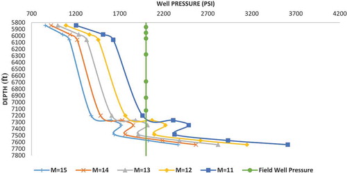
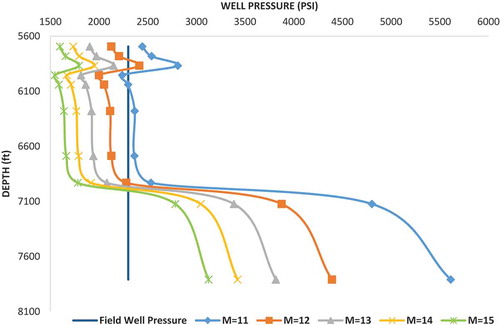
Figure 2. Sensitivity study on Hoek–Brown material constant (M) on well X2.

4.1. Parametric study of Hoek–Brown material constants on model performance

In this study, the condition for sanding is for the well flowing pressure to be at/below the value predicted using (8) (i.e., onset of shear failure). Prior to validating this model, initial rock mass condition was not known (i.e., in terms of parameter M). Therefore, the values of M were adjusted severally between 11 and 15 (which represents rock mass conditions as presented in Table 1) and subsequently used in predicting the minimum well pressure at failure for the two wells, considering the perforation depth stated earlier. From the field production data (Tables 2 and 3), the wells were reported sand producers at the field imposed well pressures. As can be seen from Figures 1 and 2, wells X1 and X2 were sand producers because the well flowing pressures (field pressures) were lowered below the minimum pressures predicted using Eq. 8 i.e., 2500 and 3467 psi for well X1 and X2, respectively (at M = 1 which is the case for sandstone reservoir rock; Table 1).

The value of M as presented in Table 1 for different rock conditions depends on mineralogy, composition and grain size of the intact rock. The parameter S is a measure of how fractured the rock is and it is related to rock mass cohesion (Hoek et al., 2002). To carry out the sensitivity studies, the value of M was adjusted between 11 and 15 as stated earlier to account for the effect of level of disturbance in the reservoir rock while keeping S at 1 for intact rocks and checking the effect on the predicted well pressures. The parameter S was consequently varied between 0 and 1 and the value of M was kept at 11 for intact rocks and its effects was observed in the calculated well pressure.

In terms of Mohr’s failure envelope, large values of M give steeply inclined Mohr envelopes and high instantaneous friction angles which make the safe region wider and this is generally found in strong brittle rocks while low values give lower instantaneous frictional angles (Hoek et al., 2002). The constant S varies as a function of how fractured the rock is, from a maximum value of 1 for intact rocks to zero for heavily fractured types where the tensile strength has dropped to zero.

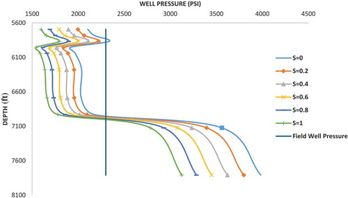
Figures 1 and 2 show the lowest well pressure achieved at the highest value of M, indicating high frictional strength and this in turn allows the well pressure to be lowered further and consequently results in a better drawdown without shear failure. Figure 3 presents the effect of variation in S on predicted well pressure. It was observed that the minimum well pressure was increasing with reducing value of S. This is in agreement classical rock physics in which reduction in rock strength corresponds to loss of cohesion/or reduction (Fjaer et al., 1992).

Figure 3. Sensitivity study on Hoek–Brown material constant (s) on well X2.

4.2. Uncertainty assessment of input parameters

In this section, analysis on how change in the input parameters for the sanding prediction model (Eq. 8) will affect the calculated well pressure is presented. To use Eq. 8, parameters of Poisson’s ratio, minimum horizontal stress, reservoir pressure (average reservoir pressure), Poro-elastic constant, and UCS need to be supplied. Availability of these data for field applications is always a challenge because of the expensive nature of the laboratory test involved. Most times, the only means to these data is well logs, which are always readily available and provide a continuous section of such data set. It is also possible that no data may be available and the only reliable source of information is from nearby well or engineering estimated data from experience. In all cases, input data uncertainties exist. A Monte Carlo simulation of the impact of these input variables on model outcome (well pressure) was performed using @Risk software developed by Palisade at a thousand iteration steps. From the simulation results, interactive Tornado plots of correlation coefficient, regression coefficient, change in output mean, regression mapped value and spider diagrams were generated, which gives indications on how sensitive the result is to a specific independent variable. To perform uncertainty analysis, the first step is to estimate the distribution of the model input parameters. Under most conditions, we just have an estimated value for a given parameter through field measurement or experience. It is very hard to know what probability distribution function a parameter satisfies. However, it is possible to know the upper and lower bounds of a specific parameter. For the case of this analysis, uniform and normal distributions were used to describe the distributions of the input parameters. The Tornado plot provides a way to clearly identify those factors whose uncertainty gives the largest impact on the output, so that operators can focus objectively on the important input variables during well assessments. Table 6 presents the range of values for the input parameters considered in the Monte Carlo simulation. The value range presented were typical upper and lower limits of the estimated input parameters as per the wells used in this study and generally represents the limit for most fields in the region. However, it could be different for other depo-belts

Table 6. Input data range for the Monte Carlo simulation

Input parameter	Value
Poisson’s ratio	0.2075–0.3425
Reservoir pressure (psi)	3090–4710
Rock strength (psi)	2964–4132
Minimum horizontal stress (psi)	4071.2–6575.2

4.3. Interpretation of the tornado plots/sensitivity analysis

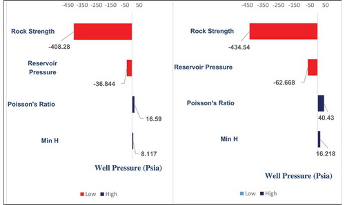
4.3.1. Effect of change in output mean

Figure 4 shows the change in output mean which is a graphical representation of the effect each input has on the output (in this case “the well pressure”) for wells X1 and X2, respectively. The inputs with larger bars generally indicate the input with the most significant effect and in that decreasing order of effect. For both wells, the rock strength (i.e., UCS) gives the most significant effect on the computed well pressure. This implies that uncertainty in rock strength value estimate will greatly affect the accuracy of the predicted well pressure, and this corresponds to the fundamentals of rock mechanics in which rocks with higher values of cohesive strength (UCS) can relatively withstand imposed stresses without failure compared to low cohesion rocks.

4.3.2. Effect of mapped coefficient value

The mapped coefficients are in units of output per standard deviation of input. For example, Input “A” has a mapped coefficient of 10,013.4, meaning that an increase of k-fraction of a standard deviation in input “A” produces an actual increase of 10,013.4 k units of the output. This value tells about the magnitude effect changes in input values have on the well pressure predicted. In Figure 5, rock strength and reservoir pressure showed a negative impact on the calculated well pressure for wells X1 and X2; this implies an inverse relationship between the calculated well pressure and rock strength/reservoir pressure; while Poisson’s ratio and minimum horizontal stress gave a direct impact on the calculated well pressures. This results give meaningful practical implications on the model performance because, rocks with higher strength can accommodate more loads and this makes the safe region on the Mohr envelope larger, as is generally found in strong brittle rocks while low strength rocks are characterized by smaller safe regions on the Mohr envelope.

Figure 4. Tornado plot of change in output mean (well pressure) for wells X1 and X2.

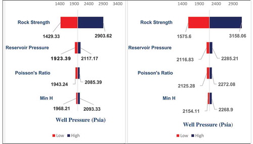
Figure 5. Tornado plot for regression-mapped value (well pressure) for wells X1 and X2.

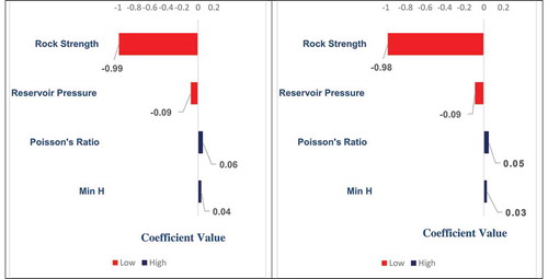
4.3.3. Effect of correlation coefficient

Generally, the correlation coefficient reveals whether increasing an input will generally decrease or increase the outcome, which then informs how consistent such trend is, however, the strength of the influence is not indicated. Therefore, the higher the correlation coefficient, the more consistently, the input increases the output (e.g., + 1 correlation coefficient implies the maximum possible correlation) while coefficient of −1 (lowest possible correlation coefficient) implies, every time the input is increased, the output is lowered. Zero correlation coefficient implies that increasing the input is just as likely as decreasing the output. Figure 6 presents the Tornado plots of correlation coefficients for wells X1 and X2, respectively. From these plots, it can be observed that rock strength and reservoir pressure have a negative correlation coefficient, which implies that every time they are increased, the predicted well pressure is lowered. The observed correlation coefficient for rock strength—0.99 and—0.98 for wells X1 and X2, respectively, shows consistency in the trend while reservoir pressure is—0.09 for both wells . Poisson’s ratio and horizontal stress both have positive correlation coefficient, which implies that an increase in both parameters will increase the well pressure predicted and in turn limits the extent to which the well pressure can be lowered without inducing shear failure.

Figure 6. Tornado plot for correlation coefficients (Spearman’s rank) for wells X1 and X2.

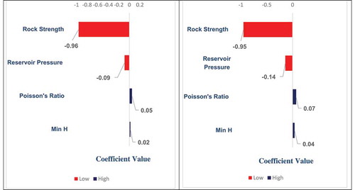
4.3.4. Effect of regression coefficient

Regression can be said to indicate the strength of the relationship between an input (independent variable) and the outcome (result). By way of example, a regression coefficient of “10” means that the output increases 10 units for a unit increase in the input while a regression coefficient of −6 indicates that the output decreases 6 units for each unit increase in the input. As evident in Figure 7, the same trend in correlation coefficient was observed in which negative coefficients were observed for rock strength and reservoir pressure while positive coefficients were seen for Poisson’s ratio and minimum horizontal stress. These can be explained that for every 1 fraction of a standard deviation increase in rock strength and reservoir pressure, the predicted well pressure will decrease by 0.96 and 0.09 standard deviation for rock strength and reservoir pressure, respectively.

Figure 7. Tornado plot for regression coefficients (well pressure) for wells X1 and X2.

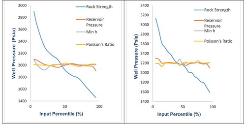
4.3.5. Spider graph

Spider graph is another visual tool used in observing the sensitivity of an output to its inputs. From the analyzed results (Figure 8), changes in calculated well pressure tend to be more sensitive to the rock strength than other input variables. This is evident in the steep slope nature of the plot of rock strength against critical well pressure and it is in conformity with the results discussed so far.

Figure 8. Spider graph of change in output mean (well pressure) for wells X1 and X2.

4.4. Effects of input parameters uncertainties on sanding onset prediction

As discussed in the work by Morita et al. (1989), sand failure envelope varies with rock strength characteristics, in-situ/borehole stress, reservoir pressure, perforation density, cavity shape, and hole angle. According to their work, sand production problems is sensitive to strength characters of the rock and in-situ stress state, but stress level in rocks is not an exclusively defined parameter without knowing the strength of the rock. In rocks shear failure envelope shifts upward with higher in-situ stress, but if the stress level can be kept below the yield strength by maintaining well pressure above the critical well pressure (predicted minimum pressure), shear failure can be delayed or avoided in oil wells. This proves why from the uncertainties study, predicted well pressure tends to be most sensitive to rock strength. For the case of reservoir pressure, depletion generally reduces reservoir pressure. Therefore, reservoir pressure depletion increases the effective stress, which results in a shift in cavity failure envelopes. This buttresses why current prediction model is equally sensitive to changes in reservoir pressure. With reservoir pressure depletion, shear-failure dominated sand problem becomes serious issue in weak/unconsolidated formation. Based on this, well pressure should be maintained above critical well pressure or drawdown reduced if a weak zone is perforated. The negligible effect of Poisson’s ratio in this study is because changes in Poisson’s ratio are down to depletion which generally alters the stress level (in this case minimum horizontal stress) in rocks. Therefore, the impact of stress level on rock yield strength should be seen as a combined effect Poisson’s ratio and horizontal stress.

5. Conclusions

In this paper, a sand predictive tool based on Hoek–Brown failure criterion was developed to study the impact of Hoek–Brown material constant and input parameters on the model performance. From the analysis, higher values of Hoek–Brown material constants M and S correspond to lower values of minimum well pressure which allows for better draw-down pressures to be achieved. The uncertainty assessment of the input parameters indicates that rock strength (UCS) has major influence on the predicted well pressure for managing the onset of sanding. From this understanding, it is recommended that accurate quantification of rock strength during drilling is essential to successful and precise assessment of sanding potential of sandstone reservoir rocks using the adopted predictive tools. Furthermore, this can help in careful selective isolation of weaker zones during well completion and if weaker zones are completed well pressure and drawdown should be managed.

Abbreviation

Min H = Min h = Minimum horizontal stress

Nomenclature

${{\sigma }_r}^{\prime }=EffectiveRadialStress$

${{\sigma }_{\theta }}^{\prime }=EffectiveTangentialStress$

${\sigma }_h=Minimumhorizontalstress$

$\nu =Poisso{n}^{\prime }sRatio$

$C_o=UniaxialCompresiveStrength$

$M=Hoek-BrownMaterialConstant\left(rockmass\right)$

$S=Hoek-BrownMaterialConstant$

$\alpha =Poro-elasticconstant$

$\bar{P}=Far-fieldporepressureorAverageReservoirPressure\left(Psi\right)$

$P_{wf}=Bottom-holeflowwingPressure\left(psi\right)$

$P_w=WellPressure\left(Psi\right)$

$GSI=GeologicStrengthindex$

$mi=Hoek-BrownMaterialConstant$

Additional information

Funding

The authors received no direct funding for this research.

Notes on contributors

Fred Temitope Ogunkunle

Fred T. Ogunkunle is currently pursuing his doctorate program in Covenant University, Ota, Nigeria. His research interests include reservoir geomechanical and its applications in drilling and post-drilling operations.

Sunday Isehunwa

Sunday Isehunwa has wide experience spanning between industry and academic environment. His research interests include routine operational reservoir engineering surveillance and support, well surveillance and performance evaluation, wellsite petroleum engineering activities during drilling operations, and solid production.

Oyinkepreye Orodu

Oyinkepreye Orodu has wide experience in Oil and Gas industry spanning field operations and academia. His research interests include “decision analysis and stochastic modeling of optimal well utilization for multi-well systems, characterization and modeling of flow units.

Seteyeobot Ifeanyi

Seteyeobot Ifeanyi is currently a lecturer at the Department of Petroleum Engineering, Covenant University, Ota, Nigeria. His research interests include pressure/rate transient analysis of horizontal wells in multilayered reservoir system and drilling fluid enhancement.

References

- Almisned , & Abdulaziz, O. (1995). A model for predicting sand production from well logging data . Doctoral Thesis. University of Oklahoma. U.S
- Araujo, E. F. , Alzate, G. A. , Arbelaez, A. , Clavijo, S. P. , Ramirez, A. C. , & Naranjo, A. (2014). Analytical prediction model of sand production integrating geomechanics for open hole and cased–perforated wells . In SPE Heavy and Extra Heavy Oil Conference: Latin America: Society of Petroleum Engineers.
- Asadi, M. S. , Khaksar, A. , Nguyen, H. Q. , & Manapov, T. F. (2017, October). Solids production prediction and management in a high porosity carbonate reservoir-a case study from offshore Vietnam . SPE/IATMI Asia Pacific oil & gas conference and exhibition . Indonesia: Society of Petroleum Engineers.
- Asadi, M. S. , Khaksar, A. , Ring, M. J. , Saric, D. , & Yin Yin, M. (2016, September). Solids production prediction and management for oil producers in highly depleted reservoirs in a Mature Malaysian field . SPE annual technical conference and exhibition . Dubai UAE: Society of Petroleum Engineers.
- Asadi, S. , Rahman, K. , Pham, H. V. , Le Minh, T. , & Butt, A. (2015). Sand production assessment considering the reservoir geomehanics and water breakthrough. The APPEA Journal , 5(01), 215–224. doi:10.1071/AJ14016
- Doust, H. , & Omatsola, E. (1990). Niger delta. In J. D. Edwards & P. A. Santogrossi (Eds.), Divergent/passive Margin Basins, AAPG Memoir 48 (pp. 239-248). Tulsa: American Association of Petroleum Geologists.
- Ekweozor, C. M. , & Daukoru, E. M. (1994). Northern delta depobelt portion of the Akata-Agbada (!) petroleum system, Niger Delta, Nigeria: Chapter 36: Part VI. Case Studies--Eastern Hemisphere.
- Fjaer, E. , Holt, R. M. , Horsud, P. , Raaen, A. R. , & Risnes, R. (1992). Petroleum related rock mechanics . Amsterdam, The Netherlands: Elsevier Science Publishers.
- Gui, F. , Khaksar, A. , Zee, W. V. D. , & Cadogan, P. (2016, October). Improving the sanding evaluation accuracy by integrating core tests, field observations and numerical simulation. In SPE Asia Pacific Oil & Gas Conference and Exhibition. Society of Petroleum Engineers.
- Hoek, E. , & Brown, E. T. (1980). Underground excavations in rock. CRC Press. Retrieved from https://content.taylorfrancis.com/books/download?dac=C2010-0-34424-2&isbn=9781482288926&format=
- Hoek, E. , Carranza-Toress, C. T. , & Corkum, B. (2002). Heok-Brown failure criterion . 5th North American Rock Mechanics Symposium (NARMS-TAC) (pp. 267–273). University of Toronto, Canadian: Toronto Press.
- Isehunwa, S. O. , Ogunkunle, T. F. , Onwuegbu, S. M. , & Akinsete, O. O. (2017). Prediction of sand production in gas and gas condensate wells. Journal of Petroleum and Gas Engineering , 8(4), 29–35. doi:10.5897/JPGE2016.0259
- Isehunwa, S. O. , & Olanrewaju, O. (2010). A simple analytical model for predicting sand production in a Niger/Delta Oil Field. International Journal of Engineering. Science & Technology , 2(9), 4379–4387.
- Kaplan, A. , Lusser, C.U. , & Norton, I.O. (1994). Tectonic map of the world, panel 10. Tulsa: American Association of Petroleum Geologists, scale1:10,000,000.
- Khaksar, A. , Taylor, P. G. , Fang, Z. , Kayes, T. , Salazar, A. , & Rahman, K. (2009). Rock strength from cores and logs: where we stand and ways to go . SPE Europe C/EAGE annual conference and exhibition (pp. 1–16). Amsterdam: Society of Petroleum Engineers.
- Klett, T. R., Ahlbrandt, T. S., Schmoker, J. W., & Dolton, G. L. (1997). Ranking of the world's oil and gas provinces by known petroleum volumes (No. 97–463). US Dept. of the Interior, Geological Survey.
- Kulke, H. (1995). Nigeria. In H. Kulke (Ed.), Regional Petroleum Geology of the World. Part II (pp. 143–172). Africa, America, Australia and Antarctica: Berlin, Gebriider Borntraeger.
- Lamorde, M. , Somerville, J. M. , & Hamilton, S. A. (2014, August). Application of the yield energy approach to prediction of sand debris production in reservoir sandstones . SPE Nigeria Annual International Conference and Exhibition . Society of Petroleum Engineers.
- Marinos, V. , Marinos, P. , & Hoek, E. (2005). The geological Strength index: Applications and limitations. Bulletin of Engineering Geology and the Environment , 64(1), 55–65. doi:10.1007/s10064-004-0270-5
- Morita, N. , Whitfill, D. L. , Fedde, O. P. , & Levik, T. (1989). Parametric study of sand production prediction: analytical approach. SPE Production Engineering , 4(01), 25–33. doi:10.2118/16990-PA
- Oyeneyin, M. B. (2005). Fines Management . SPE annual international technical conference and exhibition . Abuja: SPE.
- Tuttle, M. L. , Charpentier, R. R. , & Brownfield, M. E. (1999). The Niger Delta petroleum system: Niger Delta province, Nigeria, Cameroon, and Equatorial Guinea, Africa . US: US Department of the Interior, US Geological Survey.
- Vahidoddin, V. F. , Mahdi, M. M. , & Mehranpour, M. (2012). Sand production prediction using intelligent completion. Journal of Petroleum Science & Engineering , 2, 343–353.
- Venkitaraman, A. , Behrmann, L. A. , & Chow, C. V. (2000). Perforating requirements for sand control . SPE European petroleum conference . (pp. 1–5). France: SPE.
- World Data Atlas . (2017). Retrieved from https://knoema.com/atlas/Nigeria/topics/Energy/Gas/Reserves-of-natural-gas
- Zhang, G. , Tan, Z. , Khaksar, A. , Gui, F. , Wang, S. , White, A. , & Lei, G. (2017, October). Real-Time sanding assessment for sand-free fluid sampling in weakly consolidated reservoirs, a case study from Bohai Bay, China . SPE/IATMI Asia Pacific oil & gas conference and exhibition . Society of Petroleum Engineers.