Data clustering and imputing using a two-level multi-objective genetic algorithm (GA): A case study of maintenance cost data for tunnel fans

Abstract

This study develops a new two-level multi-objective genetic algorithm (GA) to optimise clustering to reduce and impute missing cost data for fans used in road tunnels by the Swedish Transport Administration (Trafikverket). Level 1 uses a multi-objective GA based on fuzzy c-means to cluster cost data objects based on three main indices. The first is cluster centre outliers; the second is the compactness and separation (v_k ) of the data points and cluster centres; the third is the intensity of data points belonging to the derived clusters. Our clustering model is validated using k-means clustering. Level 2 uses a multi-objective GA to impute the reduced missing cost data in volumeusing a valid data period. The optimal population has a low v_k , 0.1%, and a high intensity, 99%. It has three cluster centres, and the highest data reduction is 27%. These three cluster centres have a suitable geometry, so the cost data can be partitioned into relevant contents to be redacted for imputing. Our model shows better clustering detection and evaluation than models using k-means. The percentage of missing data for the two cost objects is the following: labour 57%, materials 81%. The second level shows highly correlated data (R-squared 0.99) after imputing. Therefore, the study concludes multi-objective GA can cluster and impute data to derive complete data for forecasting.

Keywords:

• Data clustering
• data imputing
• multi-objective GA
• fuzzy c-means
• K-means clustering

PUBLIC INTEREST STATEMENT

This research study develops a two-level model that used to cluster and impute the missing cost data for the fans of the road tunnel by the Swedish Transport Administration (Trafikverket). The two-level model uses multi-objective genetic algorithm (GA) to provide an optimal solution for the replacement time. The first level uses multi-objective GA with Fuzzy algorithm to cluster, clean and redact data. The second level used multi-objective GA to impute the missing data. Our study concludes multi-objective GA can cluster and impute data to derive complete data for forecasting and analysis.

1. Introduction

Data clustering is used to divide data as a set of objects into groups based on their similarities (Handl & Knowles, 2007; Runkler, 2012) and their sharing of relevant properties (Xu & Wunsch, 2005). Clustering is useful to explore the interrelationships between data points (Jain, Murty, & Flynn, 1999). An evaluation function can represent the data mathematically as sets, partition matrices, and/or cluster prototypes (Runkler, 2012). An evaluation function is able to measure the intrinsic properties of a partition of the data based on the compactness of the clusters and the separation between them (Handl & Knowles, 2007) to determine the quality of the partitioning (Handl & Knowles, 2007).

A difficulty of clustering is defining appropriate data clusters using multiple cluster validity indices to achieve multi solutions rather than a single solution (Deb, 2014; Saha & Bandyopadhyay, 2010). The goal of such clustering is to structure data for use in scale analysis (Xu & Wunsch, 2008). Longitudinal studies posit the existence of missing values to decrease the computational process, estimate model variables, and derive the results that would have been seen if the complete data were used. The common practice is to impute the missing data using the average of the observed values. With imputing, no values are sacrificed, thus precluding the loss of analytic results (Schafer & Graham, 2002).

A multi-objective genetic algorithm (GA) is a widely used evaluation technique to optimise clustering (Deb, Pratap, Agarwal, & Meyarivan, 2002). Multi-objective GA optimises particular functions to determine automatically the number of clusters and the partitions in a dataset simultaneously and to compute their fitness (Saha & Bandyopadhyay, 2010). It can predict missing data by finding an approximate solution interval that minimises the error prediction function (Lobato et al., 2015). Several studies of data clustering and imputing have used multi-objective GAs to understand and improve data to avoid bias in decision-making. For example, Siripen Wikaisuksakul proposed a multi-objective GA for automatic clustering in an n-dimensional database. The database is assigned a number of fuzzy groups in different dimensions using the fuzzy c-means (FCM) algorithm. This method can handle overlapping in automatic clusters by exploiting the fuzzy properties’ advantages. However, the model needs more computation time to process unlabelled data without prior knowledge (Wikaisuksakul, 2014).

Julia Handl et al. proposed a new data clustering approach, in which two or more measures of cluster quality are simultaneously optimised using a multi-objective evolutionary algorithm. The authors adapted Pareto envelope method selection for the clustering problem by incorporating specialised mutation and initialisation optimisation procedures for a number of objectives. They found this clustering approach yields high quality solutions for data clustering and greater understanding of data structure. The approach may incorporate feature selection, outlier-removal, and fixed cluster numbers (Handl & Knowles, 2004).

Lecai Cai et al. proposed a novel k-means clustering algorithm based on immune GA to improve the genetic operators for searching and clustering. They found the proposed algorithm can improve searching by adapting to different data types. Because of the high number of GA repetitions, however, the algorithm is complex (Cai, Yao, He, & Liang, 2010). Fabio Lobato et al. used multi-objective GA (MOGAImp) to impute missing data. Their model is suitable for tackling conflicting evaluation measures; it can be used for mixed-attribute datasets and takes the information from incomplete data into account by modelling. The authors suggest investigating the MOGAImp application for clustering or advanced analysis to reduce the search space and extract the knowledge required to build a model (Lobato et al., 2015). Their technique does not decrease the search space complexity.

The aim of this study is to develop a new two-level multi-objective GA to optimise clustering and impute the missing cost data of tunnel fans. The first level clusters cost data into the most relevant components and redacts the data. The second level imputes the missing cost data to create complete data for forecasting and analysis. The first level uses a multi-objective GA based on a FCM algorithm to optimise cluster centres. The selected cluster centres are optimised by considering the following: (1) cluster outliers, (2) compactness, variation between data points and clusters, and separation between clusters, and (3) intensity of data points belonging to selected clusters. The clustered data can be redacted to the relevant data points without redundancy or noise. Our module is validated using k-means clustering. In the second level, a multi-objective GA imputes the missing redacted cost data from the first level to derive complete data for forecasting. We argue that a multi-objective GA decreases the complexity, increases the flexibility, and is very effective when selecting an approximate solution interval for imputing.

2. Data collection

The study uses cost data for tunnel fans installed in Stockholm in Sweden. The data were collected over 10 years, from 2005 to 2015, by Trafikverket and are stored in a MAXIMO computerised maintenance management system (CMMS). In this CMMS, the cost data are recorded based on the work orders for the maintenance of the tunnel fans. Every work order contains corrective maintenance data, a component description, the reporting date, a problem description, and a description of the actions performed. Also included are the repair time used and the labour, material and tool cost of each work order.

In this study, we consider two cost objects, i.e. labour and materials, based on the work order input into the CMMS for the 10-year period mentioned above. We did not use the tool cost data because of the huge numbers of missing data. The selected data were clustered, filtered and imputed for the study using a multi-objective GA based on a FCM algorithm. It is important to mention that all the cost data are for real costs with no adjustment for inflation. Due to company regulations, all the cost data are encoded and expressed as currency units (cu).

3. K-means clustering

K-means algorithm divides N points in M dimensions into K clusters so that data points within the same cluster have a minimum sum of squares. The general procedure is to search for a K-partition with locally optimal within cluster by moving points from one cluster to another. The number of points in cluster C is denoted by Euclidean distance between the data point and cluster itself (Hartigan & Wong, 1979; Lohrmann & Luukka, 2018).

The data set consists of N = {1, 2, …,N} data points. Three clusters ν_i  = {1, 2, …,C} selected from the work orders of cost data portion the data into M disjoint subsets (cluster). Three clusters assumed based on many literatures. The sum of the squared Euclidean distance is used to calculate the distance between data point N and the cluster ν_i , as seen in the formula below (Likas, Vlassis, & Verbeek, 2003):

$E\left(v_i\right)=\sum _{i=1}^N\sum _{k=1}^C{N}_i-{v_k}^2$

4. Two-level system of multi-objective genetic algorithms (GAs)

The study develops a new two-level multi-objective GA, as shown in Figure 1. The GA consists of: (1) a multi-objective GA based on FCM to cluster cost data and (2) a multi-objective GA to impute missing data. In level 1, the GA is applied to the cost data objects (labour, material) at six different times (six populations) to cluster and redact data for the next level. The second level longitudinally imputes the missing data of the three cost objects. The use of two levels allows us to reduce noisy data and computational cost (Thomassey & Happiette, 2007), whilst reaching an effective and reasonable solution (Ding, Cheng, & He, 2007).

Figure 1. Two-level multi-objective GA.

4.1. Level 1: multi-objective GA based on fuzzy c-means algorithm

A multi-objective GA is widely applied in clustering because of its ability to optimise cluster centres in a large space of random populations (Deb et al., 2002). The GA operates with a population of chromosomes containing data of work orders. The cluster centres are selected randomly from the population of chromosomes. The chromosomes are proportional to the case and problem statement (Cordón, Herrera, Gomide, Hoffmann, & Magdalena, 2001).

A multi-objective GA operates on a population of cluster centre chromosomes over different generations. Over generations, chromosomes in the population are rated on their adaptation (Sortrakul, Nachtmann, & Cassady, 2005) to the new population and on their selection mechanism. Their adaptability, evaluated as the fitness function , creates the basis for a new population of chromosomes. The new population is formed using specific genetic operators, such as crossover and mutation . The fitness function is derived from the membership function (Cordón et al., 2001; Piroozfard, Wong, & Wong, 2018) using the FCM algorithm. The membership function gives cluster centre chromosomes a possible solution for the generational problem of adapting (Wikaisuksakul, 2014).

The FCM algorithm is a broad spectrum algorithm which tries to subdivide a dataset N into C pairwise disjoint subsets (cluster centres) (Bezdek, Ehrlich, & Full, 1984). This algorithm can assign data to multiple clusters. The degree of membership in the fuzzy cluster centres depends on the closeness of a given data point to a cluster centre (Izakian & Abraham, 2011). The FCM estimates the fuzzy partitions of the data and the locations of cluster centres (Hathaway & Bezdek, 2001; Lei et al., 2018). Random selection in FCM cluster centres is an iterative process yielding optimal local solutions. A multi-objective GA can process the clustering (Jain et al., 1999) by optimising the search for local optimum data points.

This paper describes a multi-objective GA based on FCM implemented six different times using a cross-validation randomisation technique. The technique aims to find the optimal cluster centre geometry with respect to the shaping of data points around cluster centres. The process is the following: a random number of cluster centres is generated randomly in each of the six implementations; the modified cluster centres are generated 25 times. The modifications are used to find the geometry of cluster centres in the cost data and determine the optimal ones. Twenty-five generations are enough for this study to obtain valid results. The following steps explain the use of the multi-objective GA.

Step 1: initial population

The cost data are a sequence of maintenance work orders; each work order is described as a chromosome and consists of a description of the work order with two cost objects: labour and materials (Z ^labour, Z ^material). The description is useful to understand the relevant data points belonging to the cluster centres.

Step 2: first multi-objective GA generation

In the first generation, the weights of each cost object are calculated in sets of N = {1, 2, …,N} data points using the Modified Adaptive Weight Approach (MAWA). MAWA is selected because it can simplify data points and efficiently calculate multi-objective GA. To calculate the weights of each cost object, we find the minimum and maximum value for each, $Z^{\mathrm{l}\mathrm{a}\mathrm{b}\mathrm{o}\mathrm{r}}=\left\{Z_{\mathrm{m}\mathrm{i}\mathrm{n}}^{\mathrm{l}\mathrm{a}\mathrm{b}\mathrm{o}\mathrm{r}},Z_{\mathrm{m}\mathrm{a}\mathrm{x}}^{\mathrm{l}\mathrm{a}\mathrm{b}\mathrm{o}\mathrm{r}}\right\}$, $Z^{\mathrm{m}\mathrm{a}\mathrm{t}\mathrm{e}\mathrm{r}\mathrm{i}\mathrm{a}\mathrm{l}}=\left\{Z_{\mathrm{m}\mathrm{i}\mathrm{n}}^{\mathrm{m}\mathrm{a}\mathrm{t}\mathrm{e}\mathrm{r}\mathrm{i}\mathrm{a}\mathrm{l}},Z_{\mathrm{m}\mathrm{a}\mathrm{x}}^{\mathrm{m}\mathrm{a}\mathrm{t}\mathrm{e}\mathrm{r}\mathrm{i}\mathrm{a}\mathrm{l}}\right\}$, and $Z^{\mathrm{t}\mathrm{o}\mathrm{o}\mathrm{l}}=\left\{Z_{\mathrm{m}\mathrm{i}\mathrm{n}}^{tool},Z_{\mathrm{m}\mathrm{a}\mathrm{x}}^{\mathrm{t}\mathrm{o}\mathrm{o}\mathrm{l}}\right\}$. The minimum and maximum values determine the relevant MAWA formula. Then, each data point in the cost object is calculated based on the conditions, as seen in the formulas below. The formulas are modified from Zheng, Ng, and Kumaraswamy (2004) to accommodate different conditions:

$\mathrm{M}\mathrm{A}\mathrm{W}\mathrm{A}\left(\mathrm{z}\right)=\frac{Z_{\mathrm{m}\mathrm{i}\mathrm{n}}\left(Z_{\mathrm{m}\mathrm{a}\mathrm{x}}-z_c\right)+\gamma }{\left(Z_{\mathrm{m}\mathrm{a}\mathrm{x}}-Z_{\mathrm{m}\mathrm{i}\mathrm{n}}\right)+\gamma },\mathrm{w}\mathrm{h}\mathrm{e}\mathrm{n}{Z}_{\mathrm{m}\mathrm{a}\mathrm{x}}\ne Z_{\mathrm{m}\mathrm{i}\mathrm{n}}$

$\mathrm{M}\mathrm{A}\mathrm{W}\mathrm{A}\left(\mathrm{z}\right)=0.1\times \frac{\left(Z_{\mathrm{m}\mathrm{a}\mathrm{x}}-z_c\right)+\gamma }{\left(Z_{\mathrm{m}\mathrm{a}\mathrm{x}}-Z_{\mathrm{m}\mathrm{i}\mathrm{n}}\right)+\gamma },\mathrm{w}\mathrm{h}\mathrm{e}\mathrm{n}{Z}_{\mathrm{m}\mathrm{i}\mathrm{n}}=0$

$\mathrm{M}\mathrm{A}\mathrm{W}\mathrm{A}\left(\mathrm{z}\right)=0.9\times \frac{\left(Z_{\mathrm{m}\mathrm{a}\mathrm{x}}-z_c\right)+\gamma }{\left(Z_{\mathrm{m}\mathrm{a}\mathrm{x}}-Z_{\mathrm{m}\mathrm{i}\mathrm{n}}\right)+\gamma },\mathrm{w}\mathrm{h}\mathrm{e}\mathrm{n}{Z}_{\mathrm{m}\mathrm{a}\mathrm{x}}=Z_{\mathrm{m}\mathrm{i}\mathrm{n}}$

γ: positive random number between 0 and 1; z_c : cost of the zth values in the current population of the object.

MAWA represents three different conditions to guide the multi-objective GA and widen the search scope. The first condition, wherein the maximum equals the minimum of the object, the weight is multiplied by 0.9. The second condition, wherein the minimum equals zero, the weight is multiplied by 0.1. The third condition, wherein the minimum does not equal the maximum, the weight depends on the current values. In these latter cases, weights can be calculated with different data types based on the maximum and minimum value for each individual object. The overall weights, as seen in the equation below, are the summation of the MAWAs of each object. This summation decreases the time required to calculate the membership function, as the evaluation has one object instead of three.

$\mathrm{M}\mathrm{A}\mathrm{W}{\mathrm{A}}_{\mathrm{o}\mathrm{v}\mathrm{e}\mathrm{r}\mathrm{a}\mathrm{l}\mathrm{l}}=\sum _m^{x=1}\mathrm{M}\mathrm{A}\mathrm{W}\mathrm{A}\left(z\right)$

m: number of objects, in this case, m = 3.

Step 3: selection

The selection of cluster centres (chromosomes) uses the chromosome pool and is directed by the concept of natural genetic systems. A random number of cluster centres, ν_i , is generated between 2 and $\sqrt{N}$. This enables the proposed clustering technique to evolve the appropriate partitioning data automatically with clusters of any shape, size, or convexity, as long as they possess some point symmetry property (Saha & Bandyopadhyay, 2010). N is the number of data points in the cost object. Cluster centres $v_i=\left\{v_1,v_2,v_3,\dots ,C\right\}$are selected and removed from N data. The selected chromosomes contain MAWA for each cost object and MAWA_overall. Noise is a random number between 0 and 1 and is added to MAWA_overall to avoid zero distance and find the relations between data points and cluster centres. The calculated fitness function defines the membership of a data point in the cluster centre. To calculate this, we need to calculate the square of the Euclidean distance ($d_{ik}^2$) between data points z_i and ν_i (Bezdek et al., 1984).

$d_{ik}^2=\sum _N^{j=1}{\left(z_{kj}-v_{ij}\right)}^2,1\le k\le N,1\le i\le C$

z_kj : object’s data points; ν_ij : cluster’s centre points.

Fitness function membership, fitness (z_ik ), is the degree of belonging of z_i to ν_i (Wikaisuksakul, 2014) and is expressed as:

$\mathrm{f}\mathrm{i}\mathrm{t}\mathrm{n}\mathrm{e}\mathrm{s}\mathrm{s}\left(z_{ik}\right)=\frac{1}{{\sum }_{j=1}^C{\left(\frac{d_{ik}}{d_{jk}}\right)}^{2/\left(m-1\right)}},1\le k\le N,1\le i\le C$

The highest fitness (z_ik ) of a data point will be in cluster centre ν_i .

The first objective of the paper is to calculate cluster centre outliers to select the best pool of cluster centres. Given the equal fitness function of each data point to the selected cluster centres, $\left\{v_1,v_2,v_3,\dots ,C\right\}$, the number of outliers should be small. In this case, the cluster outlier problem, or the error of the membership degree J(z,v) function, is expressed as the equal distance between data point z_i and cluster centres ν_i (Bezdek, 1973).

$\mathrm{J}\left(z,v\right)=\sum _{i=1}^C\sum _{k=1}^N\left(\mathrm{f}\mathrm{i}\mathrm{t}\mathrm{n}\mathrm{e}\mathrm{s}\mathrm{s}\left(z_{ik}\right)\right)d_{ik}^2$

C: number of cluster centres; N: number of data points belonging to cluster centres.

The second objective of the paper is to select the best cluster centres based on compactness and separation percentages, ν_k  (z, ν; N). Compactness measures the variation in data within a cluster or between data and cluster centroids; this variation should be kept small. Separation considers the variation between cluster centroids; this variation should be large. To obtain the best cluster centres over GA generations and to find the optimal number of clusters, we need to find the minimum percentage of ν_k (S.H. Kwon, 1998).

$v_k\left(z,v;N\right)=\frac{{\sum }_{i=1}^C{\sum }_{k=1}^N\left(\mathrm{f}\mathrm{i}\mathrm{t}\mathrm{n}\mathrm{e}\mathrm{s}\mathrm{s}\left(z_{ik}\right)\right)d_{ik}^2+\left(\frac{1}{C}\right){\sum }_{i=1}^C\parallel v_i-\bar{v}{\parallel }^{{ }^2}+\gamma }{\mathrm{m}\mathrm{i}{\mathrm{n}}_{i\ne j}\parallel v_i-v_j{\parallel }^{{ }^2}+\gamma }$

$\parallel v_i-{\bar{v}}^2\parallel$: average distance between C cluster centres; $\mathrm{m}\mathrm{i}{\mathrm{n}}_{i\ne j}\parallel v_i-{v_j}^2\parallel$: minimum distance between C cluster centres.

The average distance is used to eliminate the monotonically decreasing tendency when there are large numbers of clusters; γ is a random value between 0 and 1 to avoid division by zero.

The third objective is to measure the intensity, that is, the number of data points z_i belonging to cluster centres ν_i . This will show the cluster centres’ geometry.

Overall, these objectives are intended to facilitate the measurement of the aggregation of fuzzy membership degrees so that we may evaluate and optimise the cluster centres and find the best cluster centres in the population.

Step 4: crossover and mutation

Crossover is a probabilistic process exchanging information between two parent cluster centres (chromosomes) to generate two new child cluster centres (chromosomes). In this study, we use single point crossover with a fixed crossover probability to generate new cluster centre values because we only use two data objects (labour, material). For cluster chromosomes of length l, a crossover point is generated in the range [1, l − 2]. The chromosomes to the right of the crossover point are exchanged to produce two cluster centre offspring. The objects are connected by weight, and the value of the weight should move with the new cluster generation.

Fifty percent of the collected cluster centres randomly experience mutation. As we are considering the representation of data point values in this study, we swap between costs values for each selected work order of chromosomes after crossover.

Step 5: new generation

The new generation of cluster centres will repeat steps 3–4 continuously for 25 generations. At this point, the best fitting GA generation of cluster centres will be selected to cluster and redact data in volumewith keeping the same data parameter’s structure. Twenty-five generations are enough for these data because the fitness function value is repeated after the fifth generation. The new redacted data will not contain noise or redundant contents. They will mostly have relevant and significant data points belonging to cluster centres and should differ according to cost data description. The resulting data will be ready for the second level, imputing the missing data.

4.2. Level 2: multi-objective genetic algorithm

In this level, a multi-objective GA is applied longitudinally to the data. Multi-objective GA operates with a population of chromosomes that contains labour cost and materials cost objects. Forty percent of each cost object is selected randomly at two different times. Multi-objective GA operates on the selected population over different generations to find the appropriate cost range to impute missing data for each object. During the GA generations, chromosomes in the population are rated on their adaptation, and their selection mechanism to the new population is evaluated. Their adaptability ( fitness function ) is the basis for a new population of chromosomes. The new population is formed using specific genetic operators such as crossover and mutation . Multi-objective GA is used to fill in the zero value data from an appropriate cost range based on the best fitness function over different generations. The following steps describe level 2.

Step 1: initial population

A longitudinal study of each cost object (Z ^labour, Z ^material, Z ^tool) is used to impute missing data using multi-objective GA for the three objects in parallel.

Step 2: first GA generation and selection

The first generation is done by randomly selecting 40% of the initial population of cost objects at two different times so that 80% of the data comprise different chromosomes. We select two chromosomes to validate the GA operators. We select 80% because a high range of missing data requires us to find an appropriate range of values to impute missing data.

We find the minimum and maximum for 40% of the population and for each cost object. We generate a random number P_i between the minimum and maximum of each cost object. Data point z_i . fitness (z_i ) for each selection in each object is calculated based on the formula below (Hadavandi, Shavandi, & Ghanbari, 2011). Then, the chromosome pairs for each object are summed.

The fitness function is a statistical method finding the root mean absolute percentage error of the correlated imputed data. The lowest fitness function is selected to transform data to the next generation after the GA is applied.

$\mathrm{f}\mathrm{i}\mathrm{t}\mathrm{n}\mathrm{e}\mathrm{s}\mathrm{s}\left(z_i\right)=\sqrt{\frac{1}{N}\sum _{t=1}^N{\left(Y_i-P_i\right)}^2}$

N: number of training data; Y_i : actual value of ith training; P_i : generated value of ith training.

Step 3: crossover and mutation

In this study, we use a two-point crossover with a fixed crossover probability. For chromosomes of length l, a crossover point is generated in the range [1, 1/3 l], [1/3 l, 2/3 l], and [2/3 l, l]. The values of objects are connected and should be exchanged to produce two new offspring. We select two points to create more value ranges and find the best fit.

Fifty percent of the selected chromosomes randomly undergo mutation with the arrival of new chromosomes. For the cost object values, we swap two opposite data values.

Step 4: new generation

The new generation will repeat steps 2–3 continuously for 25 generations. Twenty-five generations are enough for these data because the fitness function increases after the fourth generation. The best fit generation will have the lowest fitness function. The selected generation is used to randomly impute new values between the selected ranges for the missing data for each cost object. This step will yield fully correlated data for better estimation of the forecasting model.

After this step, R-squared regression analysis is used to validate the imputed cost objects. R-squared gives information about the correlations of the cost values for each cost object before and after imputing.

5. Results and discussion

In what follows, we present the results of our two-level multi-objective GA.

5.1. Results of level 1: multi-objective GA based on fuzzy c-means algorithm

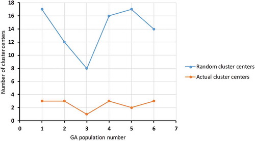
In this study, we test six populations individually using a multi-objective GA based on a FCM algorithm and compare them to optimise the cluster centres for the three different cost objects. Figure 2 shows the number of random cluster centres generated for each population with the actual cluster centres around which data points are shaped. The actual cluster centres of the generated clusters are the clusters around which the data points are shaped. In addition, the actual cluster centres (chromosomes) are modified over 25 generations of the data population. The first and second population have three actual cluster centres, created from 17 and 12 random cluster centres respectively. The third population has only one cluster centre, derived from eight random cluster centres. The fourth, fifth and sixth populations have between two and three cluster centres from 16, 17, and 14 random cluster centres respectively. The number of cluster centres is not the main criterion; rather, we are more concerned with the optimal cluster centres. The percentage of intensity for each population gives a better understanding of the cluster centres’ effectiveness.

Figure 2. Number of cluster centres for six populations.

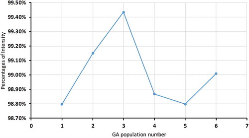
As Figure 3 shows, in the first population, 98.80% of the data belong to three cluster centres. The second population has two cluster centres, and 99.15% of the data are relevant. The third population has the highest percentage with 99.43% relevant data, but it has only one cluster centre. In this case, we cannot prove the population is optimal because one cluster centre is not enough to understand the data. The fourth and fifth populations have 98.88% and 98.8% relevant data respectively. The fifth population has only two cluster centres (the fourth has three), so it has the lowest percentage. The sixth population has 99% of the data shaped around three cluster centres. The optimal cluster centre will have the most data points shaped around it.

Figure 3. Data intensity percentages for six populations.

Cluster centre roles can be represented by the percentage of data reduction for each population. Figure 4 shows the data reduction percentages for each population after choosing and implementing the cluster centres.

Figure 4. Data reduction percentages for six populations.

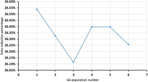
As Figure 4 shows, the first and second populations have 26.55% and 26.33% data reduction in volumerespectively. The first population has three cluster centres and the second has two. The first has the highest reduction percentage over the six populations but the lowest intensity. The third population has 26.11% reduction, the lowest percentage, but there is only one cluster centre in this population, not enough to understand the data. The fourth and fifth populations have 26.4% reduction for three and two cluster centres respectively. The last population has 26.25% reduction with three cluster centres and 99% intensity. Overall, the data redaction percentages are not high enough to determine the optimal cluster centres. This means we need to study compactness and separation (ν_k ) for the cluster centres of each population.

Figure 5 shows the ν_k percentages for each population. In this figure, a lower ν_k means lower compactness and higher separation between cluster centres. The first population has a ν_k of 0.09% over 25 generations, the lowest value. This population has three cluster centres and higher data reduction, as seen in Figures 2 and 4. The second population has higher ν_k than the first population, at 0.25%, and two cluster centres. The third has 0.11% ν_k with one cluster centre. In this case, one cluster is excluded because the separation in ν_k is zero, so it cannot be compared with other populations. The fourth and fifth populations have 1.17% and 0.09% ν_k , respectively, with two and three cluster centres, respectively, as seen in Figure 2. The highest ν_k is found in the fourth population; here, the cluster centres are almost convergent. The sixth population has the highest ν_k , 3.49%, with three cluster centres among the six populations.

Figure 5. Compactness and separation (ν_k ) percentages for six populations.

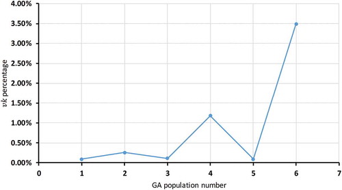
The optimal population with optimal cluster centres does not always mean the population and the cluster centres have the lowest and highest peaks for the number of cluster centres, the intensity, the data reduction percentage, or ν_k . In this study, we average the optimal cluster centres to discover most of the data points; specifically, we look at efficient intensity, high data reduction, and low ν_k of cluster centres. The error membership J(z,ν) has zero value in the proposed methodology over populations and with different multi-objective GA generations.

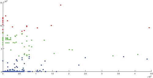
In this study, the first population has a low ν_k , 0.09%, a high percentage of intensity, 98.80%, with three cluster centres, and the highest data reduction, 26.55%, compared to other populations. These three cluster centres have a suitable geometry in the data, making most of the cost data points understandable and discoverable. Figure 6 shows the data points for the two cost objects, labour and materials, and the clustering results of the first generation with three cluster centres.

Figure 6. Data clustering of the first population.

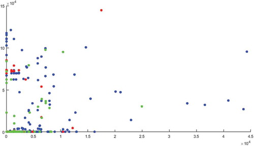
These cluster centres are used to reduce the data into relevant parts and prepare for the second level of multi-objective GA to impute the missing data. Note that Figure 6 has three different colours for the three cluster centres of the first population. The clusters distributed over the data points because the cluster centres geometry stands on optimal place. These centres make better understanding of the data points. The data are compared and evaluated to reduce the original data to the most relevant contents without redundancy or noise.

5.2. Results of level 2: genetic algorithm

The outcome of the first level, specifically in the first population, indicates the amount of missing data in the cost objects. Labour and materials costs have 56.84% and 81.02% missing data respectively. Missing data cause a substantial amount of bias, make the analysis of the data more arduous, and reduce analysis efficiency. Multi-objective GA is implemented for each cost object to impute the missing data. The imputation will help to provide complete data for better estimation of forecasting models.

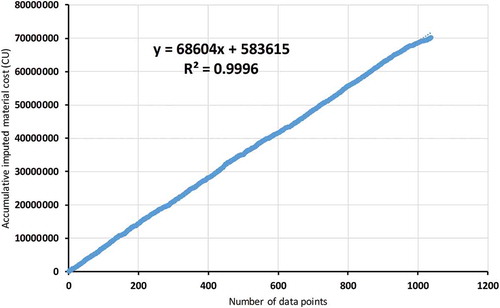
R-squared regression analysis is used to validate the imputation process using multi-objective GA and to determine the differences before and after imputation for each cost object. Figure 7 shows R-squared is 0.847 for the reduced accumulated labour cost data, and Figure 8 shows a better R-squared value, 0.9926, after imputing the missing labour cost data. This means imputing increases the correlation of the labour cost values. Figure 9 shows R-squared is 0.4401 for the accumulative materials cost before imputation; after the missing data are imputed, Figure 10 shows a higher R-squared result, 0.9996. The correlation between cost values is improved after imputation.

Figure 7. R-squared for accumulative labour cost before imputation.

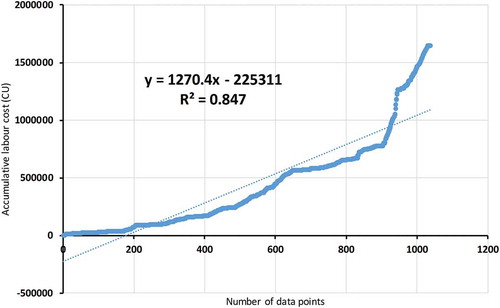
Figure 8. R-squared for accumulative labour cost after imputation.

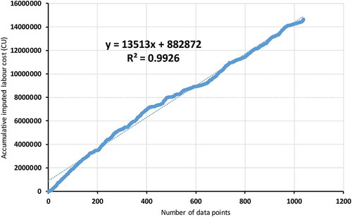
Figure 9. R-squared for accumulative materials cost before imputation.

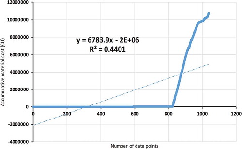
Figure 10. R-squared for accumulative materials cost after imputation.

Using multi-objective GA for each level is time consuming, even when it executes on a virtual machine of a server with special specifications. The server used in this study has 16 processors of E5-2690V2 (25M cash), 128 GB of RAM, 300 GB of Hard disk, and Windows-7 Enterprise 64 bit. Table 1 shows the time taken for clustering and imputation for each population. Clearly, clustering is more time consuming than imputation.

Table 1. Time taken for each population

GA populations	Clustering (HH:MM:SS)	Imputation (HH:MM:SS)
1	10:00:51	00:00:16
2	05:38:48	00:00:17
3	02:16:58	00:00:17
4	08:56:05	00:00:16
5	09:15:17	00:00:17
6	06:18:05	00:00:17

Unlike imputation, the time taken for clustering is dissimilar for each population; the clustering process has different calculations and comparisons based on a randomly generated number of cluster centres. The imputation process has fewer calculations and requires almost the same amount of time for each population, as the population size is always 80% of the cost data for each cost object.

6. Validation

A k-means algorithm is implemented on cost data objects to cluster data. Figure 11 shows the data points for the two cost objects, labour and materials, and the clustering results for three clusters. These clusters divide the data points into three certain partitions. The certain cluster numbers might be inaccurate, and the data need more or less cluster. In addition, the clustering does not show an understanding of the relations and correlations between the data points for labour and material costs. The data reduction will not be easy, because a cluster’s geometry might not be the optimal one.

Figure 11. K-means data clustering.

7. Conclusions

This study develops a new two-level multi-objective GA based on a FCM clustering algorithm. This GA creates a large search space for optimising cluster centres to reduce data. The algorithm gives us the ability to evaluate cost data and find suitable clustering for a problem statement. In addition, it performs well with poor data with high missing values. The optimal cluster centres are the average cluster centres with efficient intensity, high data reduction, and low ν_k . Multi-objective GA based on FCM has these advantages. In addition, our clustering model shows better results than k-means clustering.

The two-level multi-objective process is time consuming, however, and requires a special server and specifications. In addition, the algorithm needs further research to derive a rule-based system for clustering and to reduce the time required. Multi-objective GA imputing shows an optimal range of values to impute missing data. It can provide appropriate data ranges to accommodate data variations, and it shows minimum imputing errors. The correlation of cost data values after the missing data are imputed is high and relevant.

Acknowledgements

The authors gratefully acknowledge Dr. Ali Ismail Awad, Luleå University of Technology, Luleå, Sweden, for his support and for allowing us to use the computing facilities of the Information Security Laboratory to conduct the experiments in this study. This work is partially supported by the Youth Innovative Talent Project (2017KQNCX191) from the Department of Education of Guandong Province, China.

Additional information

Funding

The authors received no direct funding for this research.

Notes on contributors

Yamur K. Aldouri

Yamur K. Aldouri a Ph.D. student in operation and maintenance engineering from Luleå University of Technology, Luleå, Sweden. Currently, he is working as a data scientist in DFIND, Göteborg, Sweden. His current research interests include artificial intelligence, machine learning, eMaintenance, data mining, and Big Data analytics.

Hassan Al-Chalabi

Hassan Al-Chalabi received the Ph.D. degree in operation and maintenance engineering from Luleå University of Technology, Luleå, Sweden, in 2014. He is currently working as an Associate Senior Lecturer with the Division of Operation and Maintenance Engineering, Luleå University of Technology, Luleå, Sweden. His current research interests are mainly in Operation and Maintenance, Replacement models, Optimization aspects, Reliability Engineering and LCC analysis.

Liangwei Zhang

Liangwei Zhang received the Ph.D. degree in operation and maintenance engineering from Luleå University of Technology, Luleå, Sweden, in 2017. He is currently working as a lecturer with the Department of Industrial Engineering, School of Mechanical Engineering, Dongguan University of Technology, Dongguan, China. His current research interests include machine learning, fault detection, eMaintenance, and Big Data analytics.

References

- Bezdek, J. C . (1973). Fuzzy mathematics in pattern classification. Ph. D. Dissertation, Applied Mathematics, Cornell University.
- Bezdek, J. C. , Ehrlich, R. , & Full, W. (1984). FCM: The fuzzy c-means clustering algorithm. Computers & Geosciences , 10(2–3), 191–203. doi:10.1016/0098-3004(84)90020-7
- Cai, L. , Yao, X. , He, Z. , & Liang, X. (2010). K-means clustering analysis based on immune genetic algorithm. Paper presented at the World Automation Congress (WAC), 2010 (pp. 413–418).
- Cordón, O. , Herrera, F. , Gomide, F. , Hoffmann, F. , & Magdalena, L. (2001). Ten years of genetic fuzzy systems: Current framework and new trends. Paper presented at the Joint 9th IFSA World Congress and 20th NAFIPS International Conference, 2001 (pp. 1241–1246).
- Deb, K. (2014). Multi-objective optimization. In Search methodologies (pp. 403-449). Boston, MA: Springer.
- Deb, K. , Pratap, A. , Agarwal, S. , & Meyarivan, T. (2002). A fast and elitist multiobjective genetic algorithm: NSGA-II. IEEE Transactions on Evolutionary Computation , 6(2), 182–197. doi:10.1109/4235.996017
- Ding, C. , Cheng, Y. , & He, M. (2007). Two-level genetic algorithm for clustered traveling salesman problem with application in large-scale TSPs. Tsinghua Science & Technology , 12(4), 459–465. doi:10.1016/S1007-0214(07)70068-8
- Hadavandi, E. , Shavandi, H. , & Ghanbari, A. (2011). An improved sales forecasting approach by the integration of genetic fuzzy systems and data clustering: Case study of printed circuit board. Expert Systems with Applications , 38(8), 9392–9399. doi:10.1016/j.eswa.2011.01.132
- Handl, J. , & Knowles, J. (2004). Evolutionary multiobjective clustering. Paper presented at the International Conference on Parallel Problem Solving from Nature (pp. 1081–1091).
- Handl, J. , & Knowles, J. (2007). An evolutionary approach to multiobjective clustering. IEEE Transactions on Evolutionary Computation , 11(1), 56–76. doi:10.1109/TEVC.2006.877146
- Hartigan, J. A. , & Wong, M. A. (1979). Algorithm AS 136: A k-means clustering algorithm. Journal of the Royal Statistical Society Series C (Applied Statistics) , 28(1), 100–108.
- Hathaway, R. J. , & Bezdek, J. C. (2001). Fuzzy c-means clustering of incomplete data. IEEE Transactions on Systems, Man, and Cybernetics, Part B (Cybernetics) , 31(5), 735–744. doi:10.1109/3477.956035
- Izakian, H. , & Abraham, A. (2011). Fuzzy c-means and fuzzy swarm for fuzzy clustering problem. Expert Systems with Applications , 38(3), 1835–1838. doi:10.1016/j.eswa.2010.07.112
- Jain, A. K. , Murty, M. N. , & Flynn, P. J. (1999). Data clustering: A review. ACM Computing Surveys (CSUR) , 31(3), 264–323. doi:10.1145/331499.331504
- Kwon, S. H. (1998). Cluster validity index for fuzzy clustering. Electronics Letters , 34(22), 2176. doi:10.1049/el:19981523
- Lei, T., Jia, X., Zhang, Y., He, L., Meng, H., & Nandi, A. K . (2018). Significantly fast and robust fuzzy c-means clustering algorithm based on morphological reconstruction and membership filtering. IEEE Transactions on Fuzzy Systems.
- Likas, A. , Vlassis, N. , & Verbeek, J. J. (2003). The global k-means clustering algorithm. Pattern Recognition , 36(2), 451–461. doi:10.1016/S0031-3203(02)00060-2
- Lobato, F. , Sales, C. , Araujo, I. , Tadaiesky, V. , Dias, L. , Ramos, L. , & Santana, A. (2015). Multi-objective genetic algorithm for missing data imputation. Pattern Recognition Letters , 68, 126–131. doi:10.1016/j.patrec.2015.08.023
- Lohrmann, C. , & Luukka, P. (2018). A novel similarity classifier with multiple ideal vectors based on k-means clustering. Decision Support Systems , 111, 27–37. doi:10.1016/j.dss.2018.04.003
- Piroozfard, H. , Wong, K. Y. , & Wong, W. P. (2018). Minimizing total carbon footprint and total late work criterion in flexible job shop scheduling by using an improved multi-objective genetic algorithm. Resources, Conservation and Recycling , 128, 267–283. doi:10.1016/j.resconrec.2016.12.001
- Runkler, T. A. (2012). Data analytics: Models and algorithms for intelligent data analysis . Germany: Springer Science & Business Media.
- Saha, S. , & Bandyopadhyay, S. (2010). A symmetry based multiobjective clustering technique for automatic evolution of clusters. Pattern Recognition , 43(3), 738–751. doi:10.1016/j.patcog.2009.07.004
- Schafer, J. L. , & Graham, J. W. (2002). Missing data: Our view of the state of the art. Psychological Methods , 7(2), 147. doi:10.1037/1082-989X.7.2.147
- Sortrakul, N. , Nachtmann, H. L. , & Cassady, C. R. (2005). Genetic algorithms for integrated preventive maintenance planning and production scheduling for a single machine. Computers in Industry , 56(2), 161–168. doi:10.1016/j.compind.2004.06.005
- Thomassey, S. , & Happiette, M. (2007). A neural clustering and classification system for sales forecasting of new apparel items. Applied Soft Computing , 7(4), 1177–1187. doi:10.1016/j.asoc.2006.01.005
- Wikaisuksakul, S. (2014). A multi-objective genetic algorithm with fuzzy c-means for automatic data clustering. Applied Soft Computing , 24, 679–691. doi:10.1016/j.asoc.2014.08.036
- Xu, R. , & Wunsch, D. (2005). Survey of clustering algorithms. IEEE Transactions on Neural Networks , 16(3), 645–678. doi:10.1109/TNN.2005.845141
- Xu, R. , & Wunsch, D. (2008). Clustering . United States of America: John Wiley & Sons.
- Zheng, D. X. , Ng, S. T. , & Kumaraswamy, M. M. (2004). Applying a genetic algorithm-based multiobjective approach for time-cost optimization. Journal of Construction Engineering and Management , 130(2), 168–176. doi:10.1061/(ASCE)0733-9364(2004)130:2(168)