Simulation of three-phase induction motor using nonlinear model predictive control technique

Abstract

In this paper, nonlinear model predictive control (NMPC) has been used to control an induction motor (IM). The IM model that is used in the control is third or fifth order model that is based in the vector analysis of the IM. In the third order model, the rotor speed and fluxes are considered as system states where the source frequency and the stator currents are control variables. In the fifth order, the state variables involve stator currents, rotor speed and fluxes where the control variables are stator voltages and source frequency. The formulated nonlinear optimal control problems that are used in the NMPC frameworks are not based on the field ordination technique, however, the input frequency is computed by the MPC optimizer. Moreover, the convergence or stability of the motor speed is guaranteed using stability auxiliary constraint. Simulation studies show the performance of the proposed control algorithm.

Keywords:

• model predictive control
• optimal control
• induction motor

PUBLIC INTEREST STATEMENT

Induction motors and variable-speed drives are widely used in industrial plants since they can operate at different operating points. Normally, the field orientation control will be done by assuming one of the flux components equals to zero, so one can obtain the needed frequency.

Nonlinear model predictive control can employ an explicit nonlinear model and constraints on state and control variables.

In this work we use the original nonlinear model of the induction motor to formulate the nonlinear optimal control problem. Both flux components are not assumed to be zeros, but they are considered state variables in the nonlinear model predictive control problem. The control variables will then be the input frequency and source voltages or the frequency and source currents. The convergence or stability of the motor speed is guaranteed using stability auxiliary constraint.

1. Introduction

The induction motor (IM) and its control have been widely researched in the last three decades due to many reasons; the IM is less expensive compared to other motors types, so the IM can be used in a wide rang of applications such as heavy lifting, wind turbine and electrical vehicle. In addition, the maintenance cost can be neglected in the IM due to its construction. In other words, one can notice that a wide range of industrial drive applications use IMs (Buja & Kazmierkowski, 2; Leonhard, 2001) than other motor types. These drivers have been designed and built using the “modern” or vector modeling method. The IM vector modeling depends on two reference frames; stationary and arbitrary, which were originally introduced by Clark and Park using well-known 3-to-2 phase transformations (Clarke, 1943; Park, 15). Theses transformations as well as field orientation control (FOC) technique lead to an IM model in which we can deal with the IM similar to the DC motor (Holtz, 10). However, engineers always demand more efficient industrial drives, i.e., fast, simple and robust performance, for the IM application.

On the other hand a nonlinear model predictive control (NMPC) is one of the most important control algorithms, since we can employ an explicit nonlinear model as well as constraints on state and control variables (Diehl, Findeisen, & Schwarzkopf et al., 2002; Hong, Wang, Li, & Wozny et al., 2006; Qin & Badgwell, 2003). (Chang & Kim, 1997) have suggested a minimum-time minimum-loss speed control algorithm for IMs under FOC with IM variable constraints to obtain high performance and efficiency. (Miranda, Cort´Es, & Yuz et al., 2009) presented a predictive control algorithm that uses a state-space model.

Scoltock et al 2010have compared two MPC of IM. Namely, forced machine current control which was proposed in the early 1980s and model predictive direct torque/current control. They show through a simulation proposal that the steady-state performance of both methods is similar when the switching horizon of second method is limited. However, when the switching horizon is extended, the performance of the second method is improved. Wang and Gan (Wang & Gan, 2013) have proposed the design of gain scheduled continuous-time MPC with constraints. They used the linearized model of induction machine example to illustrate this controller.

The conventional field orientation condition concept is to make the IM emulate the separately excited DC motor as a source of adjustable torque. This will be done by assuming one of the flux components equals to zero while the motor rotating and then one can easily obtain the needed frequency for the motor operating point. However, in this work we use the original nonlinear model of the IM to formulate the nonlinear optimal control problem. That is, both flux components are not assumed to be zeros, but they are considered state variables in the NMPC problem. On the other hand, the control variables will then be the input frequency and source voltages (in the voltage-fed case) or the frequency and source currents (in the current-fed case).

This paper is organized as follows. Section 2 presents the IM nonlinear equations in a rotating $dq$ frame. Section 3 presents concept of NMPC used for IM control. Section 4 presents the problem formulation and the control objective. Sections 5 and 6 show the structures the IM-MPC controller using third order and fifth order models, respectively, which are simulated in Section 7. Finally, Section 8 concludes the paper.

2. Induction motor dynamics

An IM “T” equivalent circuit as shown in Figure 1 is represented in a rotating $dq$ frame for a three phase symmetrical IM. For a squirrel cage IM, the rotor bar ends are shorted circuit, i.e., $v_{qr}$ and $v_{dr}$ equal zero.

(1) $\frac{d{i}_{ds}}{dt}=-\left(\frac{R_s}{\sigma L_s}+\frac{1-\sigma }{\sigma L_r}\right)i_{ds}+{\omega }_s{i}_{qs}+\frac{L_m{R}_r}{\sigma L_s{L}_r^2}{\lambda }_{dr}+\frac{L_m}{\sigma L_s{L}_r}{\omega }_m{\lambda }_{qr}+\frac{1}{\sigma L_s}{v}_{ds}$(1)

(2) $\frac{d{i}_{qs}}{dt}=-{\omega }_s{i}_{ds}-\left(\frac{R_s}{\sigma L_s}+\frac{1-\sigma }{\sigma L_r}\right)i_{qs}-\frac{L_m}{\sigma L_s{L}_r}{\omega }_m{\lambda }_{dr}+\frac{L_m{R}_r}{\sigma L_s{L}_r^2}{\lambda }_{qr}+\frac{1}{\sigma L_s}{v}_{qs}$(2)

(3) $\frac{d{\lambda }_{dr}}{dt}=\frac{L_m{R}_r}{L_r}{i}_{ds}-\frac{R_r}{L_r}{\lambda }_{dr}+\left({\omega }_s-{\omega }_m\right){\lambda }_{qr}$(3)

(4) $\frac{d{\lambda }_{qr}}{dt}=\frac{L_m{R}_r}{L_r}{i}_{qs}-\left({\omega }_s-{\omega }_m\right){\lambda }_{dr}-\frac{R_r}{L_r}{\lambda }_{qr}$(4)

Figure 1. “T” equivalent circuit model of the IM: (a) in d-axis and (b) in q-axis.

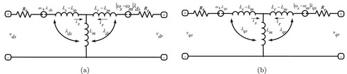
where $R_s,R_r$ are the stator and rotor resistance, respectively, $L_s,L_r$ are the stator and rotor inductance, respectively, $L_m$ is the mutual machine inductance, $v_{ds},v_{qs}$ are the $d-$ and $q-$axes stator voltage, respectively, $i_{ds},i_{qs}$ are the $d-$ and $q-$axses stator current, respectively, ${\lambda }_{ds},{\lambda }_{qs}$ are the $d-$ and $q-$axses rotor flux, respectively, ${\omega }_s,{\omega }_m$ are the synchronous and mechanical speeds, respectively. The synchronous speed is given by ${\omega }_s=\frac{2\pi f}{p}$ where $p$ is the number pole pairs. $\sigma =1-\frac{L_m^2}{L_s{L}_r}$ is called the leakage factor. For more detail on the derivation of Equations (1)–(4), the reader may refer toGehlot and Alsina (1993; Miranda et al., 2009; Ozpineci & Tolbert, 2003; Rashid, 2009). The induced torque in the IM is as follows:

$T_{ind}=\frac{3}{2}p\overrightarrow{{\lambda }_s}\otimes \overrightarrow{i_s}=\frac{3p{L}_m}{2L_r}\left(i_{qs}{\lambda }_{dr}-i_{ds}{\lambda }_{qr}\right)$

The motion equation of the rotating motor shaft is given as follows:

(5) $\frac{d{\omega }_m}{dt}=\frac{T_{ind}-T_L}{J}=\frac{3p{L}_m}{2J{L}_r}\left(i_{qs}{\lambda }_{dr}-i_{ds}{\lambda }_{qr}\right)-\frac{T_L}{J}$(5)

where $J$ is the shaft moment of inertia and $T_L$ is the load torque (Gehlot & Alsina, 1993; Miranda et al., 2009).

3. Model predictive control of the IM

MPC is a control strategy therewith we compute, online, the plant control that optimize (minimize) certain performance index subject to model equations and constrains involving states and controls (Bartholomew Biggs, 2008; Chen, O’Reilly, & Ballance, 2003; Tamimi & Li, 2009). Therefore, the model is used to predict the process output at a future time horizon by finding an optimal control sequence for a predefined objective functional using the theory of the optimal control (Camacho & Alba, 2013).

The system to be controlled is explicitly described by a set of differential algebraic equations (DAEs), e.g., (1) to (5) for the IM case, with initial conditions that are measured or estimated before optimization. Again, the optimal control is then formulated by defining a performance index to be minimized subject to the set of the DAEs, initial conditions as well as box constraints on the state and control variables. This optimal control problem must be defined along the prediction horizon, say $T_p$. Using the MPC, first part the optimal control is only applied to the plant (IM) over the control horizon $T_c$ (where $T_c<T_p$). If there are no disturbances and no model-plant mismatch then we can apply the input over the prediction horizon. But when we have disturbances and model-plant mismatches, the computed control strategy can be not realized. Therefore, a feedback mechanism will be implemented, that means, the computed open-loop input function will be implemented only until the next feedback measurements are available.

Thus, the basic structure of the MPC implementation to various dynamic processes can be shown in Figure 2(a). Figure 2(b) shows the basic principle of the MPC. We use the system model to predict the future plant outputs, based on past and current values and optimal future controls as well as the system constraints.

Figure 2. (a) Basic MPC control loop and (b) principle of model predictive control (MPC).

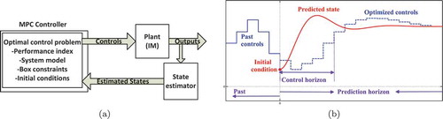
Accordingly, the MPC methodology can be summarized as follows:

1. Measure and/or estimate state variables at time instant $t_j$.

2. Compute an optimal control vector by solving an open-loop optimal control problem over a future prediction horizon subject to model equations, constrains on states and controls based on measured and/or estimated state variables.

3. Apply the first part of the computed optimal controls until the new state measurements and/or estimations are available.

4. Set $j=j+1$ and continue with step 1.

4. Problem formulation

Equations (1) to (5) represent the IM dynamics which can be rewritten in a compact form

$\frac{dx}{dt}=f(x,u)$

where $x={\left[\begin{array}{ccccc}{i}_{ds}& i_{qs}& {\lambda }_{dr}& {\lambda }_{qr}& {\omega }_m\end{array}\right]}^T$ is the state vector and $u={\left[\begin{array}{ccc}{v}_{ds}& v_{qs}& f\end{array}\right]}^T$ is the control vector; thus, the control variables of the IM are the stator voltage and source frequency. However, the IM dynamics can be reduced, namely, only Equations (3)–(5) are used to describe the IM. In this the state vector is only $x={\left[\begin{array}{ccc}{\lambda }_{dr}& {\lambda }_{qr}& {\omega }_m\end{array}\right]}^T$ and the control vector is $u={\left[\begin{array}{ccc}{i}_{ds}& i_{qs}& f\end{array}\right]}^T$, i.e., the stator currents and sources frequency are considered as control variables.

Now the control objective is to find the optimal control vector $u$, even with reduced model (Equations 3–5) or complete model (Equations 1–5), within the NMPC framework (cf. Steps 1–4, Section 3), and at the same time satisfy some constraints on the sate and control variables. In this paper, we assume only a constraint for the IM speed is only needed for the control.

5. Model predictive control of the current-fed IM

If the stator currents are the control variables of the IM, Equations (1) and (2) can be neglected. Then the reduced-order equation in the excitation reference-frame can be expressed by Equations (3)–(5). In the conventional field-oriented control, decoupling between input and output variables have been made (Chan et al., 1990). In this control strategy, the rotor flux in $q-$axis equals zero where in $d-$axis must be constant. Therefore, for given desired torque and rotor flux the stator currents and input frequency can be easily computed (Trzynadlowski, 1994).

In this work, we let all state as well as control variables be optimized in the NMPC framework. Figure 3 shows block diagram of the IM control using NMPC with considering the stator currents are the control variables. Here the state variables are the rotor fluxes which will be estimated using flux estimator, see Trzynadlowski (1994), as well as the rotor speed which will be measured. Both rotor flux estimations and rotor speed measurement will be fed back to the NMPC and considered as initial conditions each NMPC solution. On the other hand, the control variables are the stator current and operating frequency of the inverter.

Figure 3. Block diagram of the adjustable current fed IM with NMPC.

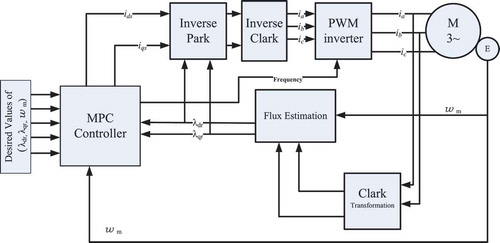
Therefore, the NOPC of the NMPC can be summarized as follows:

(6a) $\underset{i_{ds},i_{qs},f}{min}{\int }_{t_j}^{t_j+T_p}L({\lambda }_{dr},{\lambda }_{qr},{\omega }_m,i_{ds},i_{qs},f,t)dt,$(6a)

subject to

(6b) ${\lambda }_{dr}(t_j)={\lambda }_{drj},{\lambda }_{qr}(t_j)={\lambda }_{qrj},{\omega }_m(t_j)={\omega }_{mj}.$(6b)

(6c) $[i_{ds}{i}_{qs}f{]}_{min}^T\le [i_{ds}{i}_{qs}f{]}^T\le [i_{ds}{i}_{qs}f{]}_{max}^T\mathrm{\forall }t\in [t_j,t_j+T_p],$(6c)

(6d) $[{\lambda }_{dr}{\lambda }_{qr}{\omega }_m{]}_{min}^T\le [{\lambda }_{dr}{\lambda }_{qr}{\omega }_m{]}^T\le [{\lambda }_{dr}{\lambda }_{qr}{\omega }_m{]}_{max}^T\mathrm{\forall }t\in [t_j,t_j+T_p],$(6d)

and Equations (3)–(5), where Equation (6a) represents the cost functional which includes the Lagrange function $L(.)$, $t_j$ is each time instant when the states estimations and measurements are available, i.e., ${\lambda }_{drj},{\lambda }_{qrj}$ and ${\omega }_{mj}$, $j=1,2,\dots$ and $T_p$ is the prediction horizon. Equations (6d) and (6c) are called box constraint on state and control variables, respectively. Note that the control horizon $T_c=t_{j+1}-t_j$.

Without loss of generality, an additional path constraint, e.g, $s({\lambda }_{dr},{\lambda }_{qr},{\omega }_m,i_{ds},i_{qs},f,t)\ge 0\mathrm{\forall }t\in [t_j,t_j+T_p]$ can be added to Problem (6) to satisfy some torque and power rating constraint, however, this constraint is not used in our work.

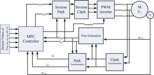
6. Model predictive control of the voltage-fed IM

In the voltage-fed IM case, the control signal for a voltage source inverter are the stator voltages. In this case, all Equations (1)–(5) are considered. This means, the stator currents, rotor voltages as well as rotor speed are considered as system states where the synchronous speed or excitation frequency is third control command that will be fed to the voltage source inverter. Figure 4 shows block diagram of the IM adjustable drive control using NMPC with voltage-fed commands.

Figure 4. Block diagram of the adjustable voltage fed IM with NMPC.

Moreover, the NOPC of the NMPC system is:

(7a) $\underset{v_{ds},v_{qs},f}{min}{\int }_{t_j}^{t_i+T_p}L(i_{ds},i_{qs},{\lambda }_{dr},{\lambda }_{qr},{\omega }_m,v_{ds},v_{qs},f,t)dt,$(7a)

subject to

(7b) $i_{ds}(t_j)=i_{dsj},i_{qs}(t_j)=i_{qsj}$(7b)

(7c) ${\lambda }_{dr}(t_j)={\lambda }_{drj},{\lambda }_{qr}(t_j)={\lambda }_{qrj}$(7c)

(7d) ${\omega }_m(t_j)={\omega }_{mj}$(7d)

(7e) $[i_{ds}{i}_{qs}f{]}_{min}^T\le [i_{ds}{i}_{qs}f{]}^T\le [i_{ds}{i}_{qs}f{]}_{max}^T\mathrm{\forall }t\in [t_j,t_j+T_p],$(7e)

(7f) $[{\lambda }_{dr}{\lambda }_{qr}{\omega }_m{]}_{min}^T\le [{\lambda }_{dr}{\lambda }_{qr}{\omega }_m{]}^T\le [{\lambda }_{dr}{\lambda }_{qr}{\omega }_m{]}_{max}^T\mathrm{\forall }t\in [t_j,t_j+T_p],$(7f)

and Equations (1)–(5), where $i_{dsj}$ and $i_{qsj}$ are the stator current measurements each time instant $t_j$ where $j=1,2,\dots$

7. Simulation results

In this section, we demonstrate the efficiency of the proposed strategy. We use an IM that has the following parameter (that is used in Trzynadlowski, 1994): Three-phase, 10 hp delta-connected, squirrel-cage IM, the stator rated voltage is 220 V, the rated frequency is 60 Hz with rated speed 1164 rpm with three pole pairs. Stator and rotor referred to stator resistances are 0.294 and 0.156Ω, respectively. Magnetizing, stator and rotor inductances are 0.041 H, 0.0424 H and 0.0417 H, respectively. Rotor moment of inertia is 0.4 $kg.m^2$.

7.1. Simulation of the current-fed IM

We apply the MPC of current-fed IM using numerical algorithm group framework (NAG) and interior point optimizer (IPOPT) which are used to combined multiple shooting and collocation on finite elements methods (Tamimi & Li, 2009). The simulation is done using I7 machine, 6 G Byte RAM and 2.6 GHz.

The control goal is to drive the IM from initial state into desired speed. Thus, to match this goal robustly, a stability constraint might be used. Therefore, we use a stability technique used in Tamimi and Li (2011) and the NOPC (6) can be be reformulated by

(8a) $\underset{i_{ds},i_{qs},f,a}{min}{\int }_{t_j}^{t_j+T_p}L({\lambda }_{dr},{\lambda }_{qr},{\omega }_m,i_{ds},i_{qs},f,a,t)dt,$(8a)

subject to constraints (6b)–(6d), and Equations (1)–(5) and

(8b) $-\zeta e^{-at}-{\omega }_m^F\le {\omega }_m(t)\le \zeta e^{-at}+{\omega }_m^F$(8b)

where $\zeta$ is called the maximum mechanical speed overshoot and be pre-defined and $a$ is the convergence rate of the mechanical speed which will be optimized. Now define $L(.)$ in (8a) by $\left(\left|\left|{\omega }_m-{\omega }_m^F|{|}_q^2+\right|\right|\zeta e^{-at}|{|}_{\hat{q}}^2\right)$ where ${\left|\left|.\right|\right|}_q^2$ is the Euclidian norm and ${\omega }_m^F$ is a desired mechanical speed and defined as 100 rad/sec. Arbitrary choosing $\zeta =110rad/sec$, $q$ and $\hat{q}$ are fixed to 0.1, prediction and control horizons are 1 and 0.1 s, respectively . ¹ Box constraints (14) and (15) are as follows: $[{\lambda }_{dr}{\lambda }_{qr}{\omega }_m{]}_{min}^T=[-2-2-160]$, $[{\lambda }_{dr}{\lambda }_{qr}{\omega }_m{]}_{max}^T=[22160]$, $[i_{ds}{i}_{qs}f{]}_{min}^T=[-90-900{]}^T$ and $[i_{ds}{i}_{qs}f{]}_{max}^T=[9090120{]}^T$. 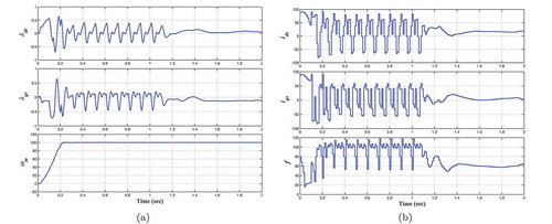The prediction horizon is divided to 100 subintervals. Figure 5(a) shows the rotor fluxes profiles and rotor speed profile, ² while Figure 5(b) shows the control profiles, i.e., stator current and excitation frequency. ³

Figure 5. (a) Rotor fluxes and speed using MPC with the current-fed control method. (b) Stator currents and excitation frequency using MPC with the current-fed control method.

Moreover, adding Inequality (8b) to OCP (6) (cf. OCP (8)) will increase the speed of convergence to the desired motor speed ensure that the desired motor speed is reached. That is, without Constraint (8b) will take more time to reach the desired motor speed. However, to solve the OCP using one of the direct methods, a discretization scheme will be used and thus the OCP is converted to a nonlinear programming (NLP) problem which will be solved usually by the method of sequential quadratic programming (SQP) (Bartholomew Biggs, 2008; Chen et al., 2003; Tamimi & Li, 2009). Without loss of generality, the size of the resulted NLP problem depends on the size of the OCP, i.e., number of control and state variables, as well as the number of subintervals used in discretization method. By adding such inequality constraints to the OCP, the number of state variables will be doubled but, however, the size of the corresponding NLP problem does not significantly increase. The reason for this observation is that the introduced inequality constraints are governed by linear, decoupled system dynamics (cf. Inequality (8b)) and, therefore, the additional size of the NLP problem comes only from the size of the vector $a$. If the combined multiple shooting-collocation approach (Tamimi & Li, 2009), for example, is used to solve the OCP (8), the inequality constraint is used to stabilize the IM speed and the number of the subinterval used to discretize the OCP is 100 subintervals, then the size of the NLP problem by adding the inequality constraint will be 607 instead of 606, see Table 1 for calculation of the NLP size. However, for the solution of OCP (8), adding these inequality constraints may cause additional computational expense due to the restriction of the system states .

Table 1. NLP size calculation of OCP (8)

Number of state variables	Number of control variables	Number of subintervals	Number of inequality constraints	NLP size ^4	NLP size ^5
$n$	$m$	$N$	$n_a$	$(N+1)(n+m)$	$(N+1)(n+m)+n_a$
3	3	100	1	606	607

7.2. Simulation of the voltage-fed IM

Again, to simulate the voltage-fed IM in Section 6, the control goal is to drive the IM into desired, $w_m^F$, speed. Thus the MPC problem is repeatedly solve the following NOPC, taking in mind the box constraint and the steady state operating point. Therefore, the nonlinear OCP can be defined as follows:

(9a) $\underset{i_{ds},i_{qs},f,a}{min}{\int }_{t_j}^{t_j+T_p}L({\lambda }_{dr},{\lambda }_{qr},{\omega }_m,i_{ds},i_{qs},f,a,t)dt,$(9a)

subject to Constraints (7b)–(6d), and Equations (1) to (5) and

(9b) $-\zeta e^{-at}-{\omega }_m^F\le {\omega }_m(t)\le \zeta e^{-at}+{\omega }_m^F$(9b)

The objective functional is also similar to that in Section 7.1. In addition, the stator voltages $v_{ds}\mathrm{a}\mathrm{n}\mathrm{d}{v}_{qs}\in [-330330]V$. Figure 6(a) shows the stator currents and rotor fluxes profiles with zero initial conditions an Figure 6(b) shows the rotor speed, stator voltages and input frequency of the IM. ⁶

Figure 6. (a) Stator currents and rotor fluxes using MPC with the voltage-fed control method. (b) Rotor speed, stator currents and excitation frequency using MPC with the voltage-fed control method.

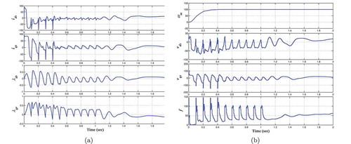
We note that, in both cases the motor speed reaches the desired speed within 0.2 s.

8. Conclusion

In this paper, NMPC is applied to control the IM. Therefore, the formulated optimal control problem (OCP) is repeatedly solved using NMPC. This OCP is first formulated using the third order IM model, thus, the system states are the fluxes in the arbitrary rotating frame as well as the motor speed where the controls are the stator currents and input frequency. The OCP is formulated using the fifth order model, i.e., the system states are the fluxes in the arbitrary rotating frame, the stator currents in the stator frame and the motor speed where the systems controls are the terminal stator voltage in the stator frame and the input frequency. These nonlinear OCPs are solved using direct method. Moreover, stabilization constraints are added the OCPs to ensure the stability of the motor speed. Simulation results show the effectiveness of the proposed controller in both cases where the motor speed reaches the desired speed after 0.2 s.

Additional information

Funding

None.

Notes on contributors

Jasem Tamimi

Jasem Tamimi is an assistant professor at the Department of Mechanical Engineering at Palestine Polytechnic University, Hebron, Palestine. His research interests include model predictive control, optimal control of electrical systems, and electrical machine control.

Notes

1. This means that the sampling rate is 0.1 s.

2. The IM initial conditions are as follows: $[{\lambda }_{drj}{\lambda }_{qrj}{\omega }_{mj}{]}^T=[000{]}^T$.

3. The piecewise constants are used to parameterize the control profiles (see Tamimi & Li, 2009).

4. Without adding inequality constraint.

5. With adding inequality constraints.

6. Piecewise constant parametrization is also used.

References

- Bartholomew Biggs, M. (2008). Nonlinear optimization with engineering applications. Springer Optimization and its Applications , 19(Springer), 1.
- Buja GS , Kazmierkowski MP. Direct torque control of pwm inverter-fed ac motors-a survey. IEEE Transactions on Industrial Electronics. 2004;51(4):744–757. doi: 10.1109/TIE.2004.831717
- Camacho, E. F. , & Alba, C. B. (2013). Model predictive control. Springer science & business media .
- Chan C , Leung W , Ng C. Adaptive decoupling control of induction motor drives. IEEE Transactions on industrial electronics. 1990;37(1):41–47. doi: 10.1109/41.45842
- Chang JH , Kim BK. Minimum-time minimum-loss speed control of induction motors under field-oriented control. IEEE transactions on industrial electronics. 1997;44(6):809– 815. doi: 10.1109/41.649942
- Chen WH , O’Reilly J , Ballance DJ. On the terminal region of model predictive control for non-linear systems with input/state constraints. International journal of adaptive control and signal processing. 2003;17:195–207. doi: 10.1002/acs.731
- Clarke, E. (1943). Circuit Analysis of AC Power Systems , 1(Wiley), 308.
- Diehl, M. , Findeisen, R. , Schwarzkopf, S. , Uslu, I. , Allgöwer, F. , Bock, H. G. , … & Schlöder, J. P. (2002). An efficient algorithm for nonlinear model predictive control of large-scale systems. Part I: Description of the Method. At Automatisierungstechnik. , 50(12), 557–567.
- Gehlot NS , Alsina PJ. A discrete model of induction motors for real-time control applications. IEEE Transactions on Industrial Electronics. 1993;40(3):317–325. doi: 10.1109/41.232211
- Holtz J. The representation of ac machine dynamics by complex signal flow graphs. IEEE transactions on industrial electronics. 1995;42(3):263–271. doi: 10.1109/41.382137
- Hong WR , Wang SQ , Li G P and Wozny , et al. A quasi-sequential approach to large-scale dynamic optimization problems. AIChE Journal 2006;52(1):255–268. doi: 10.1002/aic.10625
- Leonhard, W. (2001). Control of electrical drives (3rd ed.). Berlin: Springer Science & Business Media
- Miranda H , Cort´Es P , Yuz JI , et al. Predictive torque control of induction machines based on state-space models. IEEE Transactions on Industrial Electronics. 2009;56(6):1916– 1924. doi:10.1109/TIE.2009.2014904
- Ozpineci, B. , & Tolbert, L. M. (2003). Simulink implementation of induction machine model-a modular approach. In Electric machines and drives conference, 2003. IEMDC’03. IEEE International; Vol. 2 (pp. 728–734). Madison, WI: IEEE.
- Park RH. Two-reaction theory of synchronous machines generalized method of analysis. Part I. Transactions of the American Institute of Electrical Engineers. 1929;48(3):716–727. doi: 10.1109/T-AIEE.1929.5055275
- Qin SJ , Badgwell TA. A survey of industrial model predictive control technology. Control Engineering Practice. 2003;11(7):1096–1104. doi: 10.1016/S0967-0661(02)00186-7
- Rashid, M. H. (2009). Power electronics: Circuits, devices, and applications . England: Pearson Education India.
- Scoltock, J. , Geyer, T. , & Madawala, U. K. (2013). A comparison of model predictive control schemes for mv induction motor drives. IEEE Transactions on Industrial Informatics , 9(2), 909-919.
- Tamimi J , Li P. Nonlinear model predictive control using multiple shooting combined with collocation on finite elements. In: International Symposium on Advanced Control of Chemical Processes; July; Istanbul, Turkey. IFAC; 2009. CD Proceeding
- Tamimi, J. , & Li, P. (2011). A new optimal control formulation to ensure the stability of NMPC systems. In S.Bittanti (Ed.), 18th IFAC World Congress (pp. 5495–5500). United Kingdom: Elsevier Limitedpublisher
- Trzynadlowski, A. (1994). The field orientation principle in control of induction motors . Boston: Kluwer Academic Publishers.
- Wang L , Gan L. Gain scheduled continuous-time model predictive controller with experimental validation on ac machine. International Journal of Control. 2013;86(8):1438–1452. doi: 10.1080/00207179.2013.764019