Multioutput least square SVR-based multivariate EWMA control chart: The performance evaluation and application

Abstract

Autocorrelation leads to a bias estimator of standard control charts. It is important to develop control chart that allows autocorrelation and to evaluate its performance. The objective of this paper is to evaluate the performance of multioutput least square support vector regression (MLS-SVR)-based multivariate exponentially weighted moving average (MEWMA) control chart for monitoring multivariate autocorrelated data. For first order of vector autoregressive (VAR) and first order of vector moving average data, the proposed control chart tends to yield stable in-control average run length at about 200. The proposed control chart becomes more insensitive due to the increase of MEWMA smoothing parameter. In the real application, the proposed method is successfully applied to monitor water turbidity and chlorine residual data in the drinking water manufacturing process.

Keywords:

• autocorrelation
• average run length
• multioutput least square SVR
• multivariate EWMA control chart

PUBLIC INTEREST STATEMENT

A control chart is one of the improvement tools to monitor how a process changes over time. A good control chart will provide precise conclusion if the special causes of variation affect the actual process. The multivariate control chart for monitoring variables with time dependency has been developed. In this study, one of the multivariate control charts for monitoring autocorrelated data named MLS-SVR-based MEWMA control chart is evaluated based on two types of linear time series data. Furthermore, the proposed control chart draws a correct decision when the drinking water manufacturing process needs to be improved.

1. Introduction

Traditional control chart usually assumes that variables are statistically independent over time. However, data collected in time often show serial dependency and always affect false alarm rate and shift detection power. Consequently, a control chart developed under the assumption of independent observation would have poor performance when it is applied to monitor autocorrelated processes. To overcome this problem, researchers developed two general approaches to deal with autocorrelation in the process. First, fitting time series models to the autocorrelated data then monitoring the residuals using conventional control chart (Alwan & Roberts, 1988; Montgomery & Mastrangelo, 1991). Second, traditional control charts with modified control limits are used to monitor autocorrelated data (Lu & Reynolds, 1999; Vanbrackle & Reynolds, 1997). First approach seems to work better in high level of autocorrelation while second approach will work better in low-to-moderate level of autocorrelation (Yashchin, 1993).

Some researchers investigated the effect of autocorrelation on the control chart performance. Serially dependent data may lead to incorrect out-of-control signal and reduce the effectiveness of a control chart (Noorossana & Vaghefi, 2006). If data follow autoregressive moving average model with order (1,1), exponentially weighted moving average (EWMA) control chart will detect shift more quickly than Shewhart control chart (Wardell, Moskowitz, & Plante, 1994). Jarrett and Pan (2007) evaluated mean shift effect on the performance of multivariate control chart based on the residual of vector autoregressive (VAR) model. For small autocorrelation coefficient, Hotelling’s T ² control chart based on the residual of VAR model is effective to detect small shift of mean (Pan & Jarrett, 2007).

One of the well-known performance indicators to evaluate and to compare the effectiveness of various control charts is average run length (ARL). However, the distribution of run length is affected by serial correlation (Bagshaw & Johnson, 1975; Johnson & Bagshaw, 1974). Böhm and Hackl (1996) derived close form approximation of in-control ARL to evaluate the effect of autocorrelation on the performance of cumulative sum (CUSUM) control chart. Both Shewhart and CUSUM charts become less sensitive to detect small shift in the mean when applied to the residual of autocorrelated process (Runger, Wlllemain, & Prabhu, 1995). Kramer and Schmid (1997) evaluated the performance of residual-based multivariate exponentially weighted moving average (MEWMA) control chart for first order of bivariate VAR model. Śliwa and Schmid (2005) found that for monitoring cross-covariance purpose, residual-based MEWMA control chart has better performance than modified MEWMA control chart.

Recently, some researchers also use machine learning to improve the performance of residual-based multivariate control chart. Khediri, Weihs, and Limam (2010) studied the performances of residual-based T ², CUSUM of T ² (COT), and T ² of EWMA (EWMAT) control chart. Khediri et al. (2010) proved that multivariate control charts based on the residual of support vector regression (SVR) are more effective than multivariate control charts based on the residual of Artificial Neural Network (ANN). The SVR-based MCUSUM control chart has better performance than MCUSUM control charts based on the residual of ANN and VAR (Issam & Mohamed, 2008).

SVR is one of the machine learnings that provides global optimal solution. Meanwhile, least square SVR (LS-SVR) is least square version of standard SVR which replaces quadratic programming problem with linear programming problem (Vapnik, 1998, 1995) and changes the inequality constraints formula by the equality ones (Suykens, Gestel, Brabanter, Moor, & Vandewalle, 2002; Suykens & Vandewalle, 1999). The linear equation in LS-SVR is simple to solve and good in computational time saving. When the variables of interest are more than one, the issue becomes multioutput case. Xu, An, Qiao, Zhu, and Li (2013) introduced multioutput LS-SVR (MLS-SVR) in order to cover the Hierarchical Bayes (Heskes, 2000) intuition, where each output is permitted to have different slope function. The MLS-SVR has ability to map the multivariate input space to the multivariate output space.

Khusna, Mashuri, Suhartono, Prastyo, and Ahsan (2018) proposed MLS-SVR-based MEWMA control chart and evaluated its ability to detect the presence of both additive and innovative outliers in the simulation data which follow vector autoregressive and moving average model with order (1,1). However, the performance of MLS-SVR-based MEWMA control chart based on ARL criteria has not been investigated. Therefore, the aim of this research is to evaluate the performance of MLS-SVR-based MEWMA control chart (Khusna et al., 2018) using ARL criteria. This research calculates the ARLs using simulation studies for several combinations of smoothing parameter and multivariate linear time series data, including VAR (1) and VMA (1) model. Moreover, this research is also aimed to provide an illustrative example of MLS-SVR-based MEWMA control chart for monitoring real autocorrelated data.

The rest of this paper is organized as follows. Section 2 describes MLS-SVR-based MEWMA control chart and the way the chart is constructed. ARL algorithm is displayed at Section 3. In addition, Section 4 presents the performance of MLS-SVR-based MEWMA control chart for VAR (1) and VMA (1) data. Application of the proposed method to monitor water quality data is displayed at Section 5. Finally, some concluding remarks and future research opportunity are given in Section 6.

2. MLS-SVR-based MEWMA control chart

2.1. MLS-SVR algorithm

The standard formula of LS-SVR trains the different output in multioutput case separately. Xu et al. (2013) proposed MLS-SVR algorithm to cope the potential cross-relatedness among different output such that the relation between outputs can be captured by learning all outputs simultaneously. Let $\mathbf{Y}=[y_{ij}]\in R^{n\times \ell }$ are the observable outputs, where $i=1,2,\dots ,n$, $j=1,2,\dots ,\mathrm{\ell }$, $i$ denotes number of samples and $j$ for number of outputs. Suppose $\left\{({\mathbf{x}}_1,{\mathbf{y}}^1),({\mathbf{x}}_2,{\mathbf{y}}^2),\dots ,(\mathbf{x}{\hspace{0.17em}}_n^{\hspace{0.17em}},{\mathbf{y}}^n)\right\}$ are the specific independent and identically distributed samples, where ${\mathbf{x}}_i\in R^d$, $d$ is dimension of input, and ${\mathbf{y}}^i\in R^{\mathrm{\ell }}$.

In order to cover the Hierarchical Bayes intuition, the parameter ${\mathbf{w}}_j$ can be written as ${\mathbf{w}}_j={\mathbf{w}}_0+{\mathbf{v}}_j$. The parameter ${\mathbf{w}}_0$ describes mean vector whereas the small values of vector ${\mathbf{v}}_j$ indicate that different outputs are similar to each other. In the other words, mean vector ${\mathbf{w}}_0$ carries commonality information while vector ${\mathbf{v}}_j$ carries specialty information. Let $\phi :R^d\to R^h$ is a mapping function to higher dimensional Hilbert space with h dimension. All MLS-SVR parameters are assumed to be associated with $\phi (\mathbf{x})$ so that parameter ${\mathbf{w}}_j\in R^h(j\in N_{\mathrm{\ell }})$, vector ${\mathbf{v}}_j\in R^h(j\in N_{\mathrm{\ell }})$, and mean vector ${\mathbf{w}}_0\in R^h$.

The objective of MLS-SVR algorithm is to find the function $f(\mathbf{x})=\phi (\mathbf{x}{)}^T\mathbf{W}+(\mathbf{b}{)}^T$ which has most deviation from the actual observable outputs and at the same time is as flat as possible. On the other words, the errors are acceptable as long as the errors are less than or equal to the deviation. The flatness of function $f(\mathbf{x})$ can be obtained by looking for the small value of parameter $\mathbf{W}$. This condition is equivalent with minimizing parameter ${\mathbf{w}}_0^T{\mathbf{w}}_0$ as well as $trace\left({\mathbf{V}}^T\mathbf{V}\right)$. Therefore, estimating vector ${\mathbf{w}}_0$, matrix $\mathbf{V}=\left({\mathbf{v}}_1,{\mathbf{v}}_2,\dots ,{\mathbf{v}}_{\mathrm{\ell }}\right)\in R_{\hspace{0.17em}}^{h\times \mathrm{\ell }}$, and vector $\mathbf{b}=\left(b_1,b_2,\dots ,b_{\mathrm{\ell }}\right)\in R_{\hspace{0.17em}}^{\mathrm{\ell }}$ simultaneously could be attained by minimizing the following objective function with constraints (Xu et al., 2013):

(1) $\begin{array}{c}\mathrm{m}\mathrm{i}\mathrm{n}J({\mathbf{w}}_0,\mathbf{V},\mathbf{\Xi })=\frac{1}{2}\left({\mathbf{w}}_0^T{\mathbf{w}}_0\right)+\frac{{\gamma }^{\prime \prime }}{2\mathrm{\ell }}trace\left({\mathbf{V}}^T\mathbf{V}\right)+\frac{{\gamma }^{\prime }}{2}trace\left({\mathbf{\Xi }}^T\mathbf{\Xi }\right),\\ \mathrm{s}.\mathrm{t}\mathbf{Y}={\mathbf{Z}}^T\mathbf{W}+repmat({\mathbf{b}}^T,n,\mathbf{1})+\mathbf{\Xi },\end{array}$(1)

where matrix $\mathbf{Z}=\left(\phi \left({\mathbf{x}}_1\right),\phi \left({\mathbf{x}}_2\right),\dots ,\phi \left({\mathbf{x}}_n\right)\right)\in R^{h\times n}$, matrix $\mathbf{\Xi }=\left({\xi }_1,{\xi }_2,\dots ,{\xi }_{\mathrm{\ell }}\right)\in R_{+}^{n\times \mathrm{\ell }}$ contains slack variable, matrix $\mathbf{W}=\left({\mathbf{w}}_0+{\mathbf{v}}_1,{\mathbf{w}}_0+{\mathbf{v}}_2,\dots ,{\mathbf{w}}_0+{\mathbf{v}}_j,\dots {\mathbf{w}}_0+{\mathbf{v}}_{\mathrm{\ell }}\right)\in R^{h\times \mathrm{\ell }}$ illustrates MLS-SVR parameter, and ${\gamma }^{\prime },{\gamma }^{\prime \prime }\in R_{+}$ are regularized parameter.

The optimization problem has the assumption that it should be feasible, the function $f(\mathbf{x})$ actually exists for all approximates samples $\left\{({\mathbf{x}}_1,{\mathbf{y}}^1),({\mathbf{x}}_2,{\mathbf{y}}^2),\dots ,(\mathbf{x}{\hspace{0.17em}}_n^{\hspace{0.17em}},{\mathbf{y}}^n)\right\}$ with precision equal to an acceptable deviation. A matrix $\mathbf{\Xi }$ containing slack variable is involved in optimization problem (1) in order to cope the infeasible constraints. In addition, the regularized parameters ${\gamma }^{\prime }$ and ${\gamma }^{\prime \prime }$ describe the trade-off between the flatness of function $f(\mathbf{x})$ and the amount up to which errors larger than deviation are tolerated.

A set of dual variables is introduced in order to construct a Lagrange function from the objective function along with its constraints. The Lagrange function from the optimization problem (1) can be written as follows:

where $\mathbf{A}={\left({\alpha }_1^{\hspace{0.17em}},{\alpha }_2^{\hspace{0.17em}},\dots ,{\alpha }_{\mathrm{\ell }}^{\hspace{0.17em}}\right)}^T\in R^{n\times \mathrm{\ell }}$ contains Lagrange multiplier. According to Karush–Kuhn–Tucker method, a set of linear equation in Equation (2) yields an optimal condition.

(2) $\begin{array}{c}\mathrm{\partial }{\hspace{0.17em}}_{{\mathbf{w}}_0}^{\hspace{0.17em}}L=0\Rightarrow {\mathbf{w}}_0=\sum _{j=1}^{\mathrm{\ell }}\mathbf{Z}{\alpha }_k,\\ \mathrm{\partial }{\hspace{0.17em}}_{\mathbf{V}}^{\hspace{0.17em}}L=0\Rightarrow \mathbf{V}=\frac{\mathrm{\ell }}{{\gamma }^{\prime \prime }}\mathbf{Z}\mathbf{A},\\ \mathrm{\partial }{\hspace{0.17em}}_{\mathbf{b}}^{\hspace{0.17em}}L=0\Rightarrow {\mathbf{A}}^T{\mathbf{1}}_{\mathrm{\ell }}={\mathbf{0}}_{\mathrm{\ell }},\\ \mathrm{\partial }{\hspace{0.17em}}_{\mathbf{\Xi }}^{\hspace{0.17em}}L=0\Rightarrow \mathbf{A}=({\gamma }^{\prime })\mathbf{\Xi },\\ \mathrm{\partial }{\hspace{0.17em}}_{\mathbf{A}}^{\hspace{0.17em}}L=0\Rightarrow {\mathbf{Z}}^T\mathbf{W}+repmat\left({\mathbf{b}}^T,n,\mathbf{1}\right)+\mathbf{\Xi }-\mathbf{Y}={\mathbf{0}}_{n\times \mathrm{\ell }}.\end{array}$(2)

Following the idea of LS-SVR, the linear equation system (3) is obtained by eliminating $\mathbf{W}\mathrm{a}\mathrm{n}\mathrm{d}\mathbf{\Xi }$ matrices from Equation (2).

$\left[\begin{array}{cc}{\mathbf{0}}_{\mathrm{\ell }n\times \mathrm{\ell }}& {\mathbf{N}}_{\hspace{0.17em}}^T\\ \mathbf{N}& \mathbf{M}\end{array}\right]\left[\begin{array}{c}\mathbf{b}\\ \alpha \end{array}\right]=\left[\begin{array}{c}{\mathbf{0}}_{\mathrm{\ell }}\\ \mathbf{y}\end{array}\right],$

where matrix $\mathbf{N}=blockdiag\stackrel{\mathrm{\ell }}{\overbrace{\left({\mathbf{1}}_n,{\mathbf{1}}_n,\dots ,{\mathbf{1}}_n\right)}}\in R^{\mathrm{\ell }n\times \mathrm{\ell }}$, the positive definite matrix $\mathbf{M}=\mathbf{\Omega }+({\gamma }^{\prime }{)}^{-1}{\mathbf{I}}_{\mathrm{\ell }n}+\left(\mathrm{\ell }/{\gamma }^{\prime \prime }\right)\mathbf{Q}\in R^{\mathrm{\ell }n\times \mathrm{\ell }n}$, matrix $\mathbf{\Omega }=repmat\left(\tilde{\mathbf{K}},\mathrm{\ell },\mathrm{\ell }\right)\hspace{0.17em}\in R^{\mathrm{\ell }n\times \mathrm{\ell }n},$ matrix $\mathbf{Q}=blockdiag\stackrel{\mathrm{\ell }}{\overbrace{\left(\tilde{\mathbf{K}},\tilde{\mathbf{K}},\dots ,\tilde{\mathbf{K}}\right)}}\in R^{\mathrm{\ell }n\times \mathrm{\ell }n},$ matrix $\tilde{\mathbf{K}}={\mathbf{Z}}^T\mathbf{Z}\in R^{n\times n}$ contains kernel function, matrix $\alpha ={\left({\left({\alpha }_1^{\prime }\right)}^T,{\left({\alpha }_2^{\prime }\right)}^T,\dots ,{\left({\alpha }_{\mathrm{\ell }}^{\prime }\right)}^T\right)}^T\in R^{\mathrm{\ell }n}$ contains Lagrange multiplier, and output variables are defined with $\mathbf{y}={\left({\mathbf{y}}_1^T,{\mathbf{y}}_2^T,\dots ,{\mathbf{y}}_{\mathrm{\ell }}^T\right)}^T\in R^{\mathrm{\ell }n}$. Hence, linear equation system (3) contains $(n+1)\times \mathrm{\ell }$ equations.

However, solving linear equation system (3) directly is difficult because it is not positively definite. For this reason, linear equation system (3) is reformulated into the following one:

(4) $\left[\begin{array}{cc}\mathbf{G}& {\mathbf{0}}_{\mathrm{\ell }n\times \mathrm{\ell }n}^{\hspace{0.17em}}\\ {\mathbf{0}}_{\mathrm{\ell }\times \mathrm{\ell }}^{\hspace{0.17em}}& \mathbf{M}\end{array}\right]\left[\begin{array}{c}\mathbf{b}\\ {\mathbf{M}}^{-1}\mathbf{N}\mathbf{b}+\alpha \end{array}\right]=\left[\begin{array}{c}{\mathbf{N}}_{\hspace{0.17em}}^T{\mathbf{M}}^{-1}\mathbf{y}\\ \mathbf{y}\end{array}\right],$(4)

where $\mathbf{G}={\mathbf{N}}_{\hspace{0.17em}}^T{\mathbf{M}}^{-1}\mathbf{N}\in R^{\mathrm{\ell }\times \mathrm{\ell }}$. It can be approved that $\mathbf{G}$ is a positive definite matrix. Thus, the solutions of linear equation system (4) can be obtained using following steps:

1. Solve $\vartheta \mathrm{a}\mathrm{n}\mathrm{d}\nu$ from $\mathbf{M}\vartheta =\mathbf{N}$ and $\mathbf{M}\nu =\mathbf{y}$.

2. Calculate $\mathbf{G}={\mathbf{N}}^T\vartheta$.

3. Find solution from $\mathbf{b}={\mathbf{G}}^{-1}{\vartheta }^T\mathbf{y}$ and $\alpha =\nu -\vartheta \mathbf{b}$.

The solutions of the linear equation system (4) can be obtained by solving two linear equations which have same positive definite matrix M. Singular value decomposition is an alternative method to solve those linear equations. Supposed that $\tilde{\alpha }={\left({\left({\tilde{\alpha }}_1^{\prime }\right)}^T,{\left({\tilde{\alpha }}_2^{\prime }\right)}^T,\dots ,{\left({\tilde{\alpha }}_{\mathrm{\ell }}^{\prime }\right)}^T\right)}^T$ and $\tilde{\mathbf{b}}$ are the solutions of linear equation system (4), then the decision function of MLS-SVR can be written as follows:

$\tilde{f}(X)=\phi (X{)}^T\tilde{W}+{\left(\tilde{b}\right)}^T=\phi (X{)}^{T}repmat\left({\tilde{w}}_0,1,\mathrm{\ell }\right)+\phi (X{)}^T\tilde{V}+{\left(\tilde{b}\right)}^T$

$=\phi (X{)}^{T}repmat\left(\sum _{k=1}^{\mathrm{\ell }}\mathrm{Z}{\tilde{\alpha }}_k,1,\mathrm{\ell }\right)+\frac{\mathrm{\ell }}{{\gamma }^{\prime \prime }}\phi (X{)}^T\mathrm{Z}\left(\tilde{A}\right)+{\tilde{b}}^T$

(5) $=repmat\left(\sum _{j=1}^{\mathrm{\ell }}\sum _{i=1}^n{\tilde{\alpha }}_{ij}\tilde{k}\left(X,X_i\right),1,\mathrm{\ell }\right)+\frac{\mathrm{\ell }}{{\gamma }^{\prime \prime }}\sum _{i=1}^n{\tilde{\alpha }}_{i}K\left(X,X_i\right)+{\tilde{b}}^T$(5)

Grid search method (Hsu, Chang, & Lin, 2016) is used to identify the proper hyper-parameters of MLS-SVR. For all possible combinations of kernel function parameter, $\sigma \in \left\{2^{-15},2^{-13},\dots ,2^3\right\}$, as well as regularized parameters, ${\gamma }^{\prime \prime }\in \left\{2^{-10},2^{-8},\dots ,2^{10}\right\}$ and ${\gamma }^{\prime }\in \left\{2^{-5},2^{-3},\dots ,2^{15}\right\},$ the optimal pair of hyper-parameters $\sigma ,$ ${\gamma }^{\prime },$ and γ^” is selected based on minimum criterion from average of mean square error (MSE) over each output. An evolutionary algorithm as proposed by Härdle, Prastyo, and Hafner (2014) can also be employed to optimize SVR parameters. This might become useful for future work.

2.2. Residual-based MEWMA control chart

Let ${\mathbf{y}}_1,{\mathbf{y}}_2,\dots ,{\mathbf{y}}_{\mathrm{\ell }}$ are the observable outputs, where ${\mathbf{y}}_j=(y_{1j},y_{2j},\dots ,y_{nj}{)}^T$ with $j=1,2,\dots ,\mathrm{\ell }$, and $\mathrm{\ell }$ denotes number of outputs that satisfy multivariate autocorrelated processes. Supposed that each output has significant partial autocorrelation function until lag-$p_1,p_2,\dots ,p_{\mathrm{\ell }}$ then the inputs of MLS-SVR are selected as follows:

(6) $\mathbf{x}=\left({\mathbf{y}}_{1,(i-1)},\dots ,{\mathbf{y}}_{1,(i-p_1)},{\mathbf{y}}_{2,(i-1)},\dots ,{\mathbf{y}}_{2,(i-p_2)},\dots ,{\mathbf{y}}_{\mathrm{\ell },(i-1)},\dots ,{\mathbf{y}}_{\mathrm{\ell },(i-p_{\mathrm{\ell }})}\right).$(6)

The decision function of MLS-SVR model with optimal parameters $\hat{f}(\mathbf{x})$ is calculated using Equation (5) then the residuals are calculated as $e_{ij}=y_{ij}-\hat{f}({\mathbf{x}}_{ij})$. Hence, $n\times \mathrm{\ell }$ residual matrix $\mathbf{e}$ consists of $e_{ij},i=1,2,\dots ,n,j=1,2,\dots ,\mathrm{\ell }$.

Lowry, Woodall, Champ, and Rigdon (1992) introduced MEWMA control chart to monitor small change in the mean vector of independent observation. If the observation violates the independent assumption, then residual-based MEWMA control chart is employed. Supposed that ${\mathbf{e}}_i=(e_{i1},e_{i2},\dots ,e_{ij},\dots ,e_{i\mathrm{\ell }})$ is vector of residual from ith observation. This vector of residual is transformed to ${\mathbf{Z}}_i$ as follows:

(7) ${\mathbf{Z}}_i=\lambda {\mathbf{e}}_i+(1-\lambda ){\mathbf{Z}}_{i-1}$(7)

where $\lambda$ is smoothing parameter with $0<\lambda <1$ and initial value ${\mathbf{Z}}_0=\mathbf{0}$. The transformed value ${\mathbf{Z}}_i$ in Equation (7) is used to construct following MLS-SVR-based MEWMA statistic:

(8) $T_i^2={\mathbf{Z}}_i^T{\mathrm{\Sigma }}_{z_i}^{-1}{\mathbf{Z}}_i$(8)

where inverse covariance matrix of ${\mathbf{Z}}_i$ is calculated by ${\mathrm{\Sigma }}_{Z_i}=\frac{\lambda }{\left(2-\lambda \right)}\left[1-{\left(1-\lambda \right)}^{2i}\right]\mathrm{\Sigma }.$ In addition, $\mathrm{\Sigma }$ is covariance matrix of observation whereas $T_i^2$ in Equation (8) denotes MLS-SVR-based MEWMA statistic. The process is said to be in-control if $T_i^2$ statistic is not greater than the upper control limit (UCL), H, which refers to Prabhu and Runger (1997). Under in-control condition, the residuals of MLS-SVR model using the proper inputs selected using Equation (6) and the optimal parameters obtained as in Equation (5) are assumed to follow independent observation. Thus, the UCL of MLS-SVR residual-based MEWMA control chart is equal to the UCL of MEWMA control chart.

3. ARL algorithm

ARL is one of the well-known methods to measure and to compare the control chart performance. Run length (RL) is defined as the number of observations until the first observation is detected outside the control limits. The control chart performance could be assessed by two types of ARLs that are ARL₀ and ARL₁. The ARL₀ or in-control ARL is defined as the expected number of observations before an out-of control observation is detected when the process is actually in-control. The ARL₁ or out-of control ARL is the expected number of samples before an out of control signal is received when the process is actually shifted to an out-of-control state (Montgomery, 2009). For a fixed value of ARL₀, a chart is considered to be more effective than other charts if it has a smaller ARL₁.

There are some general methods to calculate the ARL of a control chart such as simulation, integral equation, and Markov chain approximation. Those methods had been developed by several researchers to calculate the ARL of MEWMA control chart. Lowry et al. (1992) and Linderman and Love (2000a, 2000b) calculated the ARL of MEWMA control chart using simulation. Rigdon (1995) and Bodden and Rigdon (1999) acquainted integral equation approximation to calculate the ARL of MEWMA chart. Furthermore, a Markov chain approximation for calculating the ARL of MEWMA chart is proposed by Runger and Prabhu (1996) as well as Molnau et al. (2001).

The ARLs of a control chart for time series data have a complex calculation. Śliwa and Schmid (2005) confirmed that even for univariate case, there is no explicit formula to calculate the ARL of a control chart for time series data. Kramer and Schmid (1997) and Śliwa and Schmid (2005) utilized extensive Monte Carlo simulation to determine the ARL of MEWMA control chart for time series data. In this research, the ARL of MLS-SVR-based MEWMA control chart is calculated using simulation study based on Algorithm 1.

Algorithm 1. The ARL of MLS-SVR-based MEWMA Control Chart

• 1. Specify the number of variables $\mathrm{\ell }$ and smoothing parameter $\lambda$.

• 2. Define the UCL H for specified parameters given in step 1.

• 3. Specify the parameter of multivariate linear time series data ${\mathbf{\Phi }}_p$ or ${\mathbf{\Theta }}_q$.

• 4. Generate multivariate linear time series data using parameter ${\mathbf{\Phi }}_p$ or ${\mathbf{\Theta }}_q$ given in step 3 and the residuals which satisfy multivariate normal distribution with specified mean vector ${\mu }_a=\mathbf{0}$ and covariance matrix $\mathrm{\Sigma }=\mathbf{I}$.

• 5. Train generated data resulted from step 4 using MLS-SVR algorithm, where the inputs are selected using Equation (6) and the optimal parameters along with the optimal hyper-parameters are obtained as in Equation (5).

• 6. For $C^{\prime }$ repetitions, follow these steps:

• a. Generate n samples of multivariate time series data using parameter ${\mathbf{\Phi }}_p$ or ${\mathbf{\Theta }}_q$ given in step 3 and the residuals which have mean vector ${\mu }_a=\mathbf{0}$ and covariance matrix $\mathrm{\Sigma }=\mathbf{I}$.

• b. Train the data which are generated in step 6(a) using inputs, parameters, and hyper-parameters obtained from step 5.

• c. Calculate statistics $T_i^2,i=1,2,\dots ,n$ using Equation (8).

• d. Calculate the RL, number of samples until finding the first statistic $T_i^2$ that greater than H.

• 7. Calculate ARL₀ from the average of RL over $C^{\prime }$ repetitions.

• 8. For $C^{\prime \prime }$ repetitions, where ${\mu }_a^{\prime }={\mu }_a+$mean vector shift, follow these steps:

• a. Repeat step 6 which multivariate time series data are generated with residuals that have mean vector ${\mu }_a^{\prime }$ and covariance matrix $\mathrm{\Sigma }=\mathbf{I}.$

• b. Calculate ARL₁ from the average of RL over $C^{\prime \prime }$ repetitions.

• 9. Repeat step 1 until 7 for different $\mathrm{\ell }$, $\lambda$ and the associated H.

• 10. Plot the ARL₀ and ARL₁ over the mean shift.

4. Performance evaluation of the proposed control chart

This section is aimed to investigate the performance of the proposed control chart using ARL. For this purpose, simulation studies are designed to generate multivariate linear time series data which follow VAR (1) or VMA (1) model using this mathematical expression:

(9) $\mathrm{V}\mathrm{A}\mathrm{R}(1)\hspace{0.17em}:{\mathbf{Y}}_i=\mu +{\mathbf{\Phi }}_1({\mathbf{Y}}_{i-1}-\mu )+{\mathbf{a}}_i,$(9)

(10) $\mathrm{V}\mathrm{M}\mathrm{A}(1):{\mathbf{Y}}_i=\mu +{\mathbf{a}}_i-{\mathbf{\Theta }}_1{\mathbf{a}}_{i-1},$(10)

where ${\mathbf{a}}_i$ is white noise residual which follows multivariate normal distribution with zero mean vector, ${\mu }_a={\mathbf{0}}_{\mathrm{\ell }}$, and covariance matrix $\mathrm{\Sigma }={\mathbf{I}}_{\mathrm{\ell }}$. The performance of the proposed control chart is evaluated for $\mathrm{\ell }=2$ and $\mathrm{\ell }=3$ quality characteristics. For $\mathrm{\ell }=2$ quality characteristics, the mean vector is set to be $\mu ={\left[\begin{array}{cc}{\mu }_1& {\mu }_2\end{array}\right]}^T={\left[\begin{array}{cc}5& 10\end{array}\right]}^T$. Otherwise, the mean vector is equal to $\mu ={\left[\begin{array}{ccc}{\mu }_1& {\mu }_2& {\mu }_3\end{array}\right]}^T={\left[\begin{array}{ccc}5& 10& 7\end{array}\right]}^T$. The parameters of VAR (1) and VMA (1) used in the simulation studies are shown in Table 1.

Table 1. The parameter of VAR (1) and VMA (1)

	$\mathbf{\ell }=2$	$\mathbf{\ell }=3$
VAR (1)	${\mathbf{\Phi }}_1=\left[\begin{array}{cc}{\varphi }_{11}& {\varphi }_{12}\\ {\varphi }_{21}& {\varphi }_{22}\end{array}\right]=\left[\begin{array}{cc}0.80& 0.05\\ 0.05& 0.90\end{array}\right]$	${\mathbf{\Phi }}_1=\left[\begin{array}{ccc}{\varphi }_{11}& {\varphi }_{12}& {\varphi }_{13}\\ {\varphi }_{21}& {\varphi }_{22}& {\varphi }_{23}\\ {\varphi }_{31}& {\varphi }_{32}& {\varphi }_{33}\end{array}\right]=\left[\begin{array}{ccc}0.80& 0.05& 0.05\\ 0.05& 0.90& 0.05\\ 0.05& 0.05& 0.80\end{array}\right]$
VMA (1)	${\mathbf{\Phi }}_1=\left[\begin{array}{cc}{\theta }_{11}& {\theta }_{12}\\ {\theta }_{21}& {\theta }_{22}\end{array}\right]=\left[\begin{array}{cc}0.80& 0.05\\ 0.05& 0.90\end{array}\right]$	${\mathbf{\Phi }}_1=\left[\begin{array}{ccc}{\theta }_{11}& {\theta }_{12}& {\theta }_{13}\\ {\theta }_{21}& {\theta }_{22}& {\theta }_{23}\\ {\theta }_{31}& {\theta }_{32}& {\theta }_{33}\end{array}\right]=\left[\begin{array}{ccc}0.80& 0.05& 0.05\\ 0.05& 0.90& 0.05\\ 0.05& 0.05& 0.80\end{array}\right]$

The simulation studies to calculate the ARL of the proposed control chart are carried out based on Algorithm 1 with $n=1000$ samples, $C^{\prime }=$1,000 repetitions and $C^{\prime \prime }=$14 repetitions. These simulation studies utilize the UCL which is chosen for in-control ARL equal to 200. The in-control ARL of the proposed control chart is calculated using generated in-control data which follow VAR (1) or VMA (1) model, whereas the out-of-control ARL is obtained by adding mean shift 0.2 to each residual of in-control data, i.e. ${\mu }_a^{\prime }={\mu }_a+$ mean vector shift. The multivariate linear time series data which follow VAR (1) model are modelled using MLS-SVR algorithm, where $Y_{1(i-1)}$ and $Y_{2(i-1)}$ are selected as inputs, whereas the generated data which follow VMA (1) model are modelled using $Y_{1(i-1)},Y_{1(i-2)},\dots ,Y_{1(i-10)}$ and $Y_{1(i-1)},Y_{2(i-2)},\dots ,Y_{2(i-10)}$ as the inputs in MLS-SVR algorithm. The selection of the input is based on the significance lag of partial autocorrelation function. The radial basis function (RBF) kernel function is employed in MLS-SVR modelling.

Tables 2 and 3 present the ARL of the proposed control chart for VAR (1) data with $\mathrm{\ell }=2$ and $\mathrm{\ell }=3$, respectively. For various smoothing parameters $\lambda ,$ MLS-SVR-based MEWMA control chart yields stable ARL₀ at about 200. The ARL₁ is increasing when the magnitude of smoothing parameter $\lambda$ is rising. In other words, the probability of the proposed control chart to detect a specified shift in the mean is decreasing as the increasing of the magnitude of smoothing parameter $\lambda$. Moreover, the ARL₁ is decreasing as the increasing of the mean shift. This indicates that the larger the mean shift, the faster ability of the proposed control chart to detect those actual shift.

Table 2. The ARL of the proposed control chart for VAR (1) data with $\mathrm{\ell }=2$

Mean shift	Smoothing parameter $\lambda$ (UCL)
	0.05 (7.35)	0.10 (8.64)	0.20 (9.65)	0.30 (10.08)	0.40 (10.31)	0.50 (10.44)	0.60 (10.52)	0.80 (10.58)
0.0	195.432	194.534	196.955	197.716	193.038	194.770	193.628	201.382
0.2	62.111	101.494	63.865	85.563	93.990	123.780	124.384	134.702
0.4	18.879	27.976	22.734	29.649	31.788	52.657	52.641	63.193
0.6	9.419	12.873	11.092	13.688	14.605	22.459	25.516	29.789
0.8	5.725	7.287	6.946	7.878	8.285	10.944	13.396	15.608
1.0	4.218	4.929	4.598	5.065	5.357	7.031	7.875	9.796
1.2	2.943	3.643	3.609	3.586	3.891	4.612	5.380	6.081
1.4	2.410	2.803	2.887	2.875	2.968	3.398	3.709	4.400
1.6	1.987	2.302	2.300	2.401	2.476	2.592	2.925	3.092
1.8	1.649	1.965	1.936	1.975	2.054	2.194	2.329	2.478
2.0	1.485	1.649	1.697	1.736	1.709	1.885	1.919	2.057
2.2	1.368	1.495	1.518	1.509	1.521	1.593	1.669	1.744
2.4	1.218	1.367	1.375	1.420	1.389	1.433	1.474	1.480
2.6	1.173	1.245	1.228	1.277	1.264	1.285	1.339	1.313
2.8	1.094	1.144	1.181	1.185	1.168	1.185	1.203	1.199
3.0	1.044	1.098	1.103	1.099	1.087	1.134	1.161	1.115

Table 3. The ARL of the proposed control chart for VAR (1) data with $\mathrm{\ell }=3$

Mean shift	Smoothing parameter $\lambda$ (UCL)
	0.05 (9.41)	0.10 (10.81)	0.20 (11.9)	0.30 (12.35)	0.40 (12.58)	0.50 (12.71)	0.60 (12.79)	0.80 (12.85)
0.0	190.831	192.013	197.262	197.362	203.900	202.197	196.837	196.551
0.2	44.821	49.418	70.124	59.641	88.620	124.289	131.451	145.293
0.4	14.417	16.334	20.221	19.865	29.249	49.041	64.726	74.554
0.6	7.149	8.480	9.430	10.187	13.471	18.805	27.244	35.420
0.8	4.390	5.331	5.860	5.884	7.811	8.986	13.446	16.849
1.0	3.128	3.523	3.904	4.070	4.978	5.275	6.568	8.775
1.2	2.410	2.793	2.946	3.095	3.582	3.543	3.997	5.552
1.4	1.957	2.192	2.282	2.317	2.665	2.563	2.781	3.677
1.6	1.648	1.779	1.931	1.999	2.208	2.058	2.150	2.640
1.8	1.414	1.547	1.654	1.634	1.831	1.744	1.703	2.111
2.0	1.254	1.368	1.443	1.463	1.583	1.497	1.510	1.613
2.2	1.176	1.219	1.273	1.294	1.364	1.331	1.299	1.397
2.4	1.078	1.122	1.169	1.193	1.251	1.168	1.171	1.252
2.6	1.052	1.071	1.098	1.125	1.145	1.103	1.108	1.139
2.8	1.031	1.039	1.044	1.056	1.087	1.056	1.059	1.077
3.0	1.009	1.021	1.030	1.029	1.036	1.028	1.030	1.041

The ARLs of the proposed control chart for VMA (1) data with $\mathrm{\ell }=2$ and $\mathrm{\ell }=3$ are shown by Tables 4 and 5, respectively. The proposed control chart tends to yield ARL₀ at about 200. The ARLs of the proposed control chart for VMA (1) have similar pattern with those for VAR (1) data. If the mean of each variable has shifted from 0 to 0.2, then the ARL of the proposed control chart with smoothing parameter $\lambda$ = 0.2 for monitoring VMA (1) with $\mathrm{\ell }$ = 2 variables decreases from 200 to about 150. However, the ARL of the proposed control chart for monitoring VMA (1) data with $\mathrm{\ell }$ = 3 variables diminishes from 196 to about 139 to detect that shift.

Table 4. The ARL of the proposed control chart for VMA (1) data with $\mathrm{\ell }=2$

Mean shift	Smoothing parameter $\lambda$ (UCL)
	0.05 (7.35)	0.10 (8.64)	0.20 (9.65)	0.30 (10.08)	0.40 (10.31)	0.50 (10.44)	0.60 (10.52)	0.80 (10.58)
0.0	191.528	209.450	200.855	197.182	192.157	207.018	201.489	196.645
0.2	102.481	99.689	150.308	142.579	149.902	154.908	168.190	176.479
0.4	36.124	39.184	63.490	79.445	97.133	103.503	127.560	133.873
0.6	18.967	20.904	28.430	45.911	52.547	57.546	88.078	94.690
0.8	12.351	13.128	16.808	27.673	30.440	35.718	58.271	68.000
1.0	8.811	9.057	11.192	17.812	19.439	21.353	36.545	45.659
1.2	6.631	7.080	7.927	12.675	12.706	14.073	25.118	33.433
1.4	5.154	5.530	6.615	9.752	9.167	10.402	16.800	21.784
1.6	4.155	4.346	4.863	7.062	7.159	7.269	11.822	15.606
1.8	3.564	3.796	4.121	6.087	5.528	5.634	8.453	11.410
2.0	2.930	3.174	3.492	4.912	4.680	4.577	6.961	9.186
2.2	2.450	2.780	2.798	4.277	3.921	3.562	5.284	7.104
2.4	2.145	2.426	2.479	3.738	3.172	3.076	4.598	5.683
2.6	1.895	2.146	2.189	3.258	2.847	2.579	3.626	4.699
2.8	1.776	1.988	1.921	2.931	2.534	2.257	3.042	3.676
3.0	1.606	1.766	1.747	2.644	2.157	1.953	2.742	3.177

Table 5. The ARL of the proposed control chart for VMA (1) data with $\mathrm{\ell }=3$

Mean shift	Smoothing parameter $\lambda$ (UCL)
	0.05 (9.41)	0.10 (10.81)	0.20 (11.9)	0.30 (12.35)	0.40 (12.58)	0.50 (12.71)	0.60 (12.79)	0.80 (12.85)
0.0	195.872	210.231	196.055	195.429	209.942	203.506	194.486	190.051
0.2	92.936	116.680	139.969	157.858	178.459	184.604	178.316	182.577
0.4	36.082	44.680	73.573	111.413	137.050	148.439	150.332	167.394
0.6	18.760	23.992	40.047	70.143	84.013	110.885	115.314	137.174
0.8	12.716	15.186	23.313	45.452	57.504	78.676	77.957	108.204
1.0	9.263	11.019	15.442	27.668	36.516	54.794	61.504	90.722
1.2	7.254	8.006	11.135	18.472	24.962	37.455	40.961	67.690
1.4	5.612	6.770	8.149	13.825	17.412	25.201	29.017	51.550
1.6	4.794	5.690	6.796	9.836	12.638	19.328	20.683	36.996
1.8	3.996	4.743	5.470	8.384	9.365	14.044	14.784	27.976
2.0	3.562	4.035	4.682	6.624	7.603	10.770	11.025	21.127
2.2	2.971	3.462	3.921	5.710	6.339	8.557	8.528	16.110
2.4	2.635	2.961	3.391	4.760	5.223	7.106	6.877	13.217
2.6	2.252	2.638	3.016	4.166	4.449	5.714	5.798	10.981
2.8	2.102	2.451	2.655	3.619	3.868	4.965	4.458	8.562
3.0	1.893	2.219	2.487	3.156	3.301	4.290	3.882	6.937

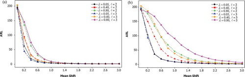
The ARLs comparison for VAR (1) and VMA (1) data is exhibited at Figure 1. The smaller the smoothing parameter $\lambda$, the faster ability of the proposed control chart to detect an actual mean shift of a process. If the mean shift of each variable has shifted from 0 to 0.2, then the ARL of the proposed control chart for monitoring VAR (1) data with $\lambda$ = 0.05 diminishes to about 50. Otherwise, the ARL of the proposed control chart for monitoring VMA (1) data with $\lambda$ = 0.05 decreases to about 100 to detect the same mean shift of a process. This indicates that the proposed control chart for monitoring VAR (1) data is more sensitive than that for monitoring VMA (1) data. Moreover, the plots of ARL for monitoring VMA (1) data with $\lambda$ = 0.05 are significantly different with those with $\lambda$ = 0.8. Hence, the performance of the proposed control chart to detect mean shift of VMA (1) data depends much on smoothing parameter $\lambda$. On the contrary, the smoothing parameter $\lambda$ does not play a significant role to the ARL of the proposed control chart for VAR (1) data.

Figure 1. The ARLs comparison of the proposed control chart for (a) VAR (1) and (b) VMA (1) data.

5. Application

In this section, the proposed control chart is applied to monitor water quality data in Surabaya, Indonesia. Two important quality characteristics in drinking water manufacturing process are water turbidity and chlorine residual. Turbidity is measured by the concentration of dissolution and the presence of particles in a liquid using Nephelometric Turbidity Units (NTU). Chlorination or affixing chlorine in to contaminated water is intended primarily for microbes killing, where chlorine residual is measured in ppm unit. Drinking water would be safe from bacteria if it has minimum chlorine residual of 0.2 ppm. However, excessive chlorine addition would affect the smell and the taste of water. Figure 2 displays time series plots of water turbidity and chlorine residual for Phase I monitoring process. Those variables are measured hourly from 19 August 2016 until 29 August 2016.

Figure 2. Time series plots of (a) hourly water turbidity data and (b) hourly chlorine residual data in Phase I.

Water quality data displayed at Figure 2 are modelled using MLS-SVR algorithm, where $Y_{1(i-1)},Y_{1(i-2)},Y_{1(i-7)},Y_{1(i-8)}$ and $Y_{2(i-1)},Y_{2(i-3)},Y_{2(i-9)}$ are selected as input variables. These inputs are chosen by considering the significant lags of partial autocorrelation function. MLS-SVR modelling using RBF kernel function yields the optimal combination of hyper parameters ${\gamma }^{\prime }=2^{-5}$, ${\gamma }^{\prime \prime }=2^{-8}$, and $\sigma =2^3$. The residuals of MLS-SVR model satisfy multivariate normal distribution and white noise condition with minimum MSE equal to 0.000605. Furthermore, these residuals are monitored using MEWMA control chart with significance level $\alpha =0.005$ and smoothing parameter $\lambda =0.2$ as displayed at Figure 3. It can be shown that MLS-SVR-based MEWMA control chart for Phase I monitoring process fulfils in-control condition. Thus, the optimal combination of hyper parameters and the control limit can be applied in Phase II monitoring process.

Figure 3. MLS-SVR-based MEWMA control chart for water quality data in Phase I.

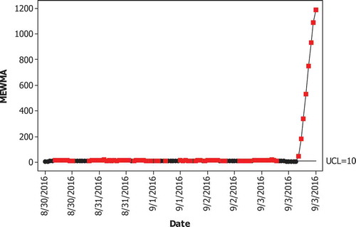
Time series plots of water turbidity and chlorine residual data for Phase II monitoring process are displayed at Figure 4. Both variables are measured in 5 days starting from 30 August 2016. It can be known that the time series plots for first four days in Phase II monitoring process follow the same pattern as the time series plots of water quality data in Phase I. However, time series plots for last day in Phase II monitoring process, starting from 10.00 AM, show unusual pattern. Time series plot of water turbidity indicates increasing pattern while time series plot of chlorine residual exhibits steep shift pattern.

Figure 4. Time series plots of (a) hourly water turbidity data and (b) hourly chlorine residual data in Phase II.

The water quality data displayed at Figure 4 are then modelled using MLS-SVR algorithm using the optimal combination of hyper parameters obtained from Phase I monitoring process. The MLS-SVR-based MEWMA control chart for Phase II monitoring process is shown at Figure 5. The residuals resulted from Phase II monitoring process do not satisfy white noise condition. Consequently, it leads to many false alarms and tight control limit. The increasing pattern far away from control limit in last eight observations indicates a serious problem in water quality data. Hence, monitoring water quality data using MLS-SVR-based MEWMA control chart becomes an early warning such that water manufacturing process needs to be improved. Looking for the assignable causes is needed in order to improve the manufacturing process. In 3 September 2016, leak pipeline is found in one of the water distribution area. Moreover, pipeline maintenance process and flow meter installation are started at 08.00 PM. As a result, both water turbidity and chlorine residual plots indicate unusual pattern.

Figure 5. MLS-SVR-based MEWMA control chart for water quality data in Phase II.

The MLS-SVR-based MEWMA control chart for water quality data needs to be updated in order to fit the next Phase I monitoring process. This step could be solved by replacing original unusual pattern with predicted value as displayed at Figure 6. Data displayed at Figure 6 are then modelled using MLS-SVR algorithm as testing data. Furthermore, white noise residuals resulted from this process are monitored using MEWMA control chart. Figure 7 shows MLS-SVR-based MEWMA control chart for updated water quality data. All of the observations fulfil in-control condition such that this control chart could be fitted as the next Phase I monitoring process.

Figure 6. Time series plots of (a) updated hourly water turbidity data and (b) updated hourly chlorine residual data in Phase II.

Figure 7. MLS-SVR-based MEWMA control chart for updated water quality data in phase II.

6. Conclusions and future research

The performance of MLS-SVR-based MEWMA control chart for monitoring multivariate linear time series data which follow VAR (1) and VMA (1) model is investigated using ARL criteria. The smaller the smoothing parameter, the more sensitive of the proposed control chart to detect an actual mean shift of a process. For a certain value of smoothing parameter, the proposed control chart for monitoring VAR (1) data is more sensitive than that for monitoring VMA (1) data. The ARLs of the proposed control chart for monitoring VMA (1) data depend much on the smoothing parameter. In addition, monitoring hourly water quality data using MLS-SVR-based MEWMA control chart becomes an early warning to improve drinking water manufacturing process if the actual assignable causes are occurred. Developing the theoretical ARL formula for MLS-SVR-based MEWMA control chart is one of the open future research topics. Bootstrap resampling method (Khusna, Mashuri, Ahsan, Suhartono, & Prastyo, 2018) and kernel density estimation (Ahsan, Mashuri, Kuswanto, Prastyo, & Khusna, 2018a, 2018b) are two computational techniques which can be used to develop the more accurate control limit of the proposed chart. Furthermore, the mixed monitoring scheme as demonstrated by Ahsan, Mashuri, Kuswanto, Prastyo, and Khusna (2018b) can also be considered for future development of this proposed chart.

Correction

This article has been republished with minor changes. These changes do not impact the academic content of the article.

Acknowledgements

The authors thank to the referees and the editor for their valuable comments and suggestions that have improved this manuscript to a better scientific level.

Additional information

Funding

This work was supported by Research, Technology, and Higher Education Ministry, Republic of Indonesia through PMDSU scheme: [Grant Number 128/SP2H/PTNBH/DRPM/2018].

Notes on contributors

Muhammad Mashuri

The corresponding author, Dr. Muhammad Mashuri, is an associate professor in the Department of Statistics, Institut Teknologi Sepuluh Nopember, Surabaya, Indonesia. His research interest includes statistical quality control and multivariate analysis, especially in industrial field. Dr. Suhartono and Dr. Dedy Dwi Prastyo are senior lecturers whose research interest includes time series analysis as well as machine learning. Hidayatul Khusna and Muhammad Ahsan are PhD students through Master Program of Education Leading to Doctoral Degree for Excellent Graduates (PMDSU), an accelerated programme for undergraduate prepared to be candidate lecturers or researchers with doctoral degrees.

References

- Ahsan, M. , Mashuri, M. , Kuswanto, H. , Prastyo, D. D. , & Khusna, H. (2018a). T2 Control Chart based on Successive Difference Covariance Matrix for Intrusion Detection System. In Journal of Physics: Conference Series (Vol. 1028, p. 12220). IOP Publishing
- Ahsan, M.,Mashuri, M., Kuswanto, H., Prastyo, D. D., & Khusna, H. (2018b). Multivariate Control Chart based on PCA Mix for Variable and Attribute Quality Characteristics.Production & Manufacturing Research, 6(1), 364–384. doi: 10.1080/21693277.2018.1517055
- Alwan, L. C. , & Roberts, H. V. (1988). Time-Series process modeling for statistical control. Journal of Business Economics and Statistics , 6(1), 87–95.
- Bagshaw, M. , & Johnson, R. A. (1975). The effect of serial correlation on the performance of CUSUM tests II. Technometrics , 17(1), 73–80. doi:10.1080/00401706.1975.10489274
- Bodden, K. M. , & Rigdon, S. E. (1999). A program for approximating the in-control ARL for the MEWMA chart. Journal of Quality Technology , 31(1), 120–123. doi:10.1080/00224065.1999.11979902
- Böhm, W. , & Hackl, P. (1996). The effect of serial correlation on the in-control average run length of cumulative score charts. Journal of Statistical Planning and Inference , 54(1), 15–30. doi:10.1016/0378-3758(95)00153-0
- Härdle, W. K. , Prastyo, D. D. , & Hafner, C. M. (2014). Support vector machines with evolutionary model selection for default prediction. In The oxford handbook of applied nonparametric and semiparametric econometrics and statistics . New York, NY: Oxford University Press.
- Heskes, T. M. (2000). Empirical Bayes for Learning to Learn . San Francisco: Morgan Kaufmann.
- Hsu, C. W. , Chang, C. C. , & Lin, C. J. (2016). A practical guide to support vector classication . Taipei: National Taiwan University.
- Issam, B. K. , & Mohamed, L. (2008). Support vector regression based residual MCUSUM control chart for autocorrelated process. Applied Mathematics and Computation , 201(1–2), 565–574. doi:10.1016/j.amc.2007.12.059
- Jarrett, J. E. , & Pan, X. (2007). The quality control chart for monitoring multivariate autocorrelated processes. Computational Statistics and Data Analysis , 51(8), 3862–3870. doi:10.1016/j.csda.2006.01.020
- Johnson, R. A. , & Bagshaw, M. (1974). The effect of serial correlation on the performance of CUSUM tests. Technometrics , 16(1), 103–112. doi:10.1080/00401706.1974.10489155
- Khediri, I. B. , Weihs, C. , & Limam, M. (2010). Support vector regression control charts for multivariate nonlinear autocorrelated processes. Chemometrics and Intelligent Laboratory Systems , 103(1), 76–81. doi:10.1016/j.chemolab.2010.05.021
- Khusna, H., Mashuri, M., Ahsan, M., Suhartono., & Prastyo, D. D. (2018). Bootstrap based maximum multivariate CUSUM control chart. Quality Technology & Quantitative Management. https://doi.org/10.1080/16843703.2018.1535765
- Khusna, H., Mashuri, M., Suhartono, Prastyo, D. D., & Ahsan, M. (2018). Multioutput least square SVR based multivariate EWMA control chart. Journal of Physics: Conference Series, 1028, 12221. IOP Publishing.
- Kramer, H. G. , & Schmid, L. V. (1997). Ewma charts for multivariate time series. Sequential Analysis , 16(2), 131–154. doi:10.1080/07474949708836378
- Linderman, K. , & Love, T. E. (2000a). Economic and economic statistical designs for MEWMA control charts. Journal of Quality Technology , 32(4), 410–417. doi:10.1080/00224065.2000.11980026
- Linderman, K. , & Love, T. E. (2000b). Implementing economic and economic statistical designs for MEWMA charts. Journal of Quality Technology , 32(4), 457–463. doi:10.1080/00224065.2000.11980032
- Lowry, C. A. , Woodall, W. H. , Champ, C. W. , & Rigdon, S. E. (1992). A multivariate exponentially weighted moving average control chart. Technometrics , 34(1), 46–53. doi:10.2307/1269551
- Lu, C. W. , & Reynolds, M. R. (1999). Control charts for monitoring the mean and variance of autocorrelated processes. Journal of Quality Technology , 31(3), 259–274. doi:10.1080/00224065.1999.11979925
- Molnau, W. E. , Runger, G. C. , Montgomery, D. C. , Skinner, K. R. , Loredo, E. N. , & Prabhu, S. S. (2001). A program for ARL calculation for multivariate EWMA charts. Journal of Quality Technology , 33(4), 515–521. doi:10.1080/00224065.2001.11980109
- Montgomery, D. C. (2009). Introduction to statistical quality control . New York, NY: John Wiley & Sons.
- Montgomery, D. C. , & Mastrangelo, C. M. (1991). Some statistical process-control methods for autocorrelated data. Journal of Quality Technology , 23(3), 179–193. doi:10.1080/00224065.1991.11979321
- Noorossana, R. , & Vaghefi, S. J. M. (2006). Effect of autocorrelation on performance of the MCUSUM control chart. Quality and Reliability Engineering International , 22(2), 191–197. doi:10.1002/(ISSN)1099-1638
- Pan, X. , & Jarrett, J. (2007). Using vector autoregressive residuals to monitor multivariate processes in the presence of serial correlation. International Journal of Production Economics , 106(1), 204–216. doi:10.1016/j.ijpe.2006.07.002
- Prabhu, S. S. , & Runger, G. C. (1997). Designing a multivariate EWMA control chart. Journal of Quality Technology , 29(1), 8. doi:10.1080/00224065.1997.11979720
- Rigdon, S. E. (1995). An integral equation for the in-control average run length of a multivariate exponentially weighted moving average control chart. Journal of Statistical Computation and Simulation , 52(4), 351–365. doi:10.1080/00949659508811685
- Runger, G. C. , & Prabhu, S. S. (1996). A markov chain model for the multivariate exponentially weighted moving averages control chart. Journal of the American Statistical Association , 91(436), 1701–1706. doi:10.1080/01621459.1996.10476741
- Runger, G. C. , Willemain, T. R. , & Prabhu, S. (1995). Average run lengths for cusum control charts applied to residuals. Communications in Statistics - Theory and Methods , 24(1), 273–282. doi:10.1080/03610929508831487
- Śliwa, P. , & Schmid, W. (2005). Monitoring the cross-covariances of a multivariate time series. Metrika , 61(1), 89–115. doi:10.1007/s001840400326
- Suykens, J. A. K. , Gestel, T. V. , Brabanter, J. D. , Moor, B. D. , & Vandewalle, J. (2002). Least squares support vector machines . Singapore: World Scientific.
- Suykens, J. A. K. , & Vandewalle, J. (1999). Least squares support vector machine classifiers. Neural Processing Letters , 9(3), 293–300. doi:10.1023/A:1018628609742
- Vanbrackle, L. N. , & Reynolds, M. R. (1997). EVVMA and cusum control charts in the presence of correlation. Communications in Statistics - Simulation and Computation , 26(3), 979–1008. doi:10.1080/03610919708813421
- Vapnik, V. N. (1995). The nature of statistical learning theory . New York, NY: Springer.
- Vapnik, V. N. (1998). Statistical learning theory . New York, NY: John Wiley & Sons.
- Wardell, D. G. , Moskowitz, H. , & Plante, R. D. (1994). Run-length distributions of special-cause control charts for correlated processes. Technometrics , 36(1), 3–17. doi:10.1080/00401706.1994.10485393
- Xu, S. , An, X. , Qiao, X. , Zhu, L. , & Li, L. (2013). Multi-output least-squares support vector regression machines. Pattern Recognition Letters , 34(9), 1078–1084. doi:10.1016/j.patrec.2013.01.015
- Yashchin, E. (1993). Performance of CUSUM control schemes for serially correlated observations. Technometrics , 35(1), 37–52. doi:10.1080/00401706.1993.10484992