Two-stage optimization model for process/supplier selection, component allocation, and quality improvement

Abstract

A company has to produce a product that gives better value than its competitors. It means the company has to produce a better quality product with lower manufacturing cost. Outsourcing has become a common practice in manufacturing where a company outsources some of their needed components to the suppliers. Supplier selection is not an easy task since it will determine the manufacturing cost and quality of the product. In this research, we develop a two-stage optimization model to help decision maker in determining the optimal suppliers which will give least manufacturing cost and how to improve the quality of the components. In the first stage, a process/supplier selection model was developed to determine the optimal tolerance and component allocation to minimize manufacturing cost and quality loss. In the second stage, investment allocation model was developed to improve the quality of the components. The objective function of the second model is to maximize the return on investment (ROI). The implementation and analysis of the proposed model were demonstrated using a simple assembly product which consists of three components and solved using Oracle Crystal Ball software.

Keywords:

• two-stage optimization
• process/supplier selection
• quality improvement
• component allocation

PUBLIC INTEREST SATEMENT

This paper deals with the make or buy decision and quality improvement that must be performed continuously by a company in order to maintain its competitiveness in the market. Hence, in this paper two optimization models are developed. The first model is used to make decision about which component that must be manufactured using company’s own facilities and which one that must be outsourced. The model also concerns with the component allocation to the respective machine/suppliers. The second model deals with the quality improvement through learning investments. The model determines the amount of investments that must be placed by the manufacturing company to improve components quality at certain level to maximize Return on Investment (ROI). Both models assume that all the investments are provided by the manufacturing company. In real context, the investments must be provided by each party involved. Hence, this consideration must be included in our further research.

1. Introduction

In an intense competition, a manufacturing company must build a competitive advantage by creating better value product than its competitors. Better product value means offering better quality product at a lower price. Lower product price can be achieved by reducing both direct and indirect costs. In a mechanical assembly product, tolerance of the component will determine the manufacturing cost. It is well known in manufacturing process that tighter tolerance will result in higher manufacturing cost with lower quality loss. Hence, the company must be able to balance both manufacturing cost dan quality loss. After determining the component tolerance or product, the company must assign the required process needed to manufacture the components by selecting the appropriate machine with good process capability.

Beside process capability, the manufacturer must consider machine’s production capacity to manufacture the certain number of components/products. Hence, not all components can be produced using the available machines and the company must make decisions about the manufacturing methods through make or buy analysis. Three strategies can be taken by a manufacturing company to provide the needed components: in-house production, outsource to suppliers, or mixed between in-house and outsource. Outsourcing has become a common practice in manufacturing. The company does not need to purchase a new machine and train the employees to operate the new machine. The outsourcing also gives many benefits to the company such as reducing production cost, doubling before tax income, increasing performance, and helping company to be more focus to its core business (Barthelemy and Adsit, 2003). Hence, the company must select several suppliers from a set of suppliers which offer better quality product at competitive price. Component or product allocation is the subsequent problem following supplier selection where the company must allocate the needed components to the selected machines/suppliers by taking into considerations several constraints such as process capability, technological capability, and production capacity.

Several models have been developed to solve suppliers selection and order allocation. For example, Rosyidi, Murtisari, and Jauhari (2016a) developed an optimization model to concurrently determine optimal suppliers and order allocation to minimize manufacturing cost and fuzzy quality loss. The model has been extended by Pratama and Rosyidi (2017) to include in-house production decision. Hence, the needed components were not only outsourced but also produced in-house. The latter model was developed in make to order environment with more complex problems due to its characteristics in producing high variety components with low volume. The objective function of the model was to minimize manufacturing cost, quality loss, and lateness cost.

All the above models only discussed about how to find the optimal combination of outsource and in-house production decisions including the components allocation to the selected process/supplier. To maintain the competitiveness of a product in the market, the manufacturing company has to continuously maintain and improve the quality of the product. Hence, the manufacturer must make some investments to purchase new machines or other production equipments and trains the employees to improve their skills. Ganeshan, Kulkarni, and Boone (2001) developed an optimization model to determine the optimal investment to improve a certain manufacturing process. They used an exponential function to relate the quality improvement with the investment cost. Chen and Tsou (2003) developed an optimization model to improve the quality of a process by balancing the investment cost and the revenue increment resulted from the improvement. Later, Tsou and Chen (2005) developed an optimization model to determine the optimal investment cost and then applied the model to improve the quality of a car seat assembly. While both models discussed optimal investment cost in a manufacturing company, several researches have been conducted to determine optimal quality investment cost by involving the learning process of suppliers. Plante (2000) and Moskowitz, Plante, and Tang (2001) developed models to improve the quality of a product through optimal allocation of variance reduction target in the supplier side. Based on both models, Rosyidi, Jauhari, Suhardi, and Hamada (2016b) developed an optimization model to determine optimal quality investment to maximize return on investment (ROI).

Generally, manufacturing companies produce their needed components using their own facilities. Hence, they have to find one or more appropriate machines or processes that give the least manufacturing cost and quality loss. An early research in this field was done by Chase, Greenwood, Loosli, and Hauglund (1990). They developed an optimization model to optimally select machine/process to minimize manufacturing cost by considering the quality requirement in term of assembly tolerance. Later, Feng, Wang, and Wang (2001) added quality loss to the research of Chase et al. (1990) as the objective function. The model was developed to simultaneously determine the optimal component tolerances through supplier selection. The model only allowed one supplier selected for each component assuming that the selected supplier has enough capacity to supply the needed components. Based on that model, Rosyidi, Murtisari, and Jauhari (2017) developed an optimization model similar to Feng et al. (2001) by allowing more than one supplier selected and including the fuzzy quality loss to accommodate uncertainty in the quality level.

There will be another important decision following the supplier selection, namely component allocation to the selected process/supplier. Several research have been conducted in supplier selection and order allocation. For example, Ghorbeni, Bahrami, and Arabzad (2012) developed a two-phase optimization model in supplier selection and order allocation. In the first phase, the supplier was selected using SWOT analysis and the weight was determined using Shannon’s Enthropy. In the second phase, an integer linear programming was used to allocate the order. Using the similar approach, Fors, Harraz, and Abouli (2011) developed a two-phased model in supplier selection and order allocation. In the first phase, a shortlist of suppliers was determined by the decision maker using several criteria. In the second phase, an optimization model was developed to select suppliers and allocate the order to the selected suppliers. The objective function of the model was to minimize total cost comprising of delivery cost, quality cost, and purchasing cost. The other research have been conducted by Rosyidi et al. (2016a) and Pratama and Rosyidi (2017) who developed optimization models to determine simultaneously the optimal process/supplier selection and allocation of each component to the selected process/supplier. If the company mixed their production methods between in-house and outsource, then component allocation becomes an important issue for manufacturing company to efficiently producing their needed components. Hence, the manufacturer and suppliers must continuously improve their processes and technological capabilities. The quality improvement is important to increase customer satisfaction. The knowledge of the manufacturer and suppliers to solve the production process problems will have a significant effect on their capability in quality improvement. The knowledge is acquired through learning process of the operators.

According to Lapre, Mukherjee, and Van Wassenhove (2000) learning process can be divided into two categories, namely conceptual learning and operational learning. Conceptual learning deals with the acquisition of know-why, while the operational learning deals with the acquisitions of know-how. Learning can also be partitioned into two categories: autonomous and induced learning (Adler & Clark, 1991). Autonomous learning stems from the production through the learning by doing, while the induced learning stems from the process improvement effort (Bernstein & Kok, 2009). Quality improvement programs are needed to train the employees to acquire the knowledge through learning process. The programs need investments in term of technology or operator trainings. Learning curve is important in this context to help the decision maker in determining optimal investment allocation.

From the above discussions, the decision making in process/supplier selection along with components allocation have been modelled separately with the decision making in quality improvement. Hence, the aim of this research is to develop two-stage optimization models which can be used to simultaneously determine optimal process/supplier along with the allocation of components to the selected process/supplier. Afterwards, the allocation of learning investment must be made by the manufacturer to improve the quality of its product. The quality improvement can be achieved by improving the component manufacturing process both in manufacturer’s and suppliers sides through investments in the learning process.

The rest of this paper has the following structure. Section 2 presents the literature review, problem definition and notations are given in Section 3. Model formulation is given in Section 4. Numerical example and analysis are given in Section 5. The conclusions and suggestions for further research are given in Section 6.

2. Problem definition and notations

A manufacturing company provides the needed components for the assembly of its final product through in-house production, outsource, or mix between in-house and outsource. Hence, an optimization model is needed to help the company determine optimal decisions about those three production modes. The decision variables of this first model include optimal components tolerance, process/supplier selection, and components allocation to the selected process/suppliers. The objective function of the model is to minimize manufacturing cost and quality loss. The second model deals with quality improvement, in which the company provides some investment fund to improve the quality both in manufacturer and suppliers sides. The decision variables of the second model are the investment allocation to the selected process/suppliers. Figure 1 shows the schematic diagram of the system under consideration. We assume that each component has the same opportunity to be produced using in-house or outsource modes. For in-house case, each component has different process routing through several processes which carried in several cells. For example, the process routing of Component 1 is Cell 1, Cell 2, and Cell 3, while Component 2 has different process routing through Cell 3, Cell 2, and Cell 1. Each cell consists of the same machines of a certain type with certain process capabilities and capacities. For outsourcing case, the component has the same opportunity to be supplied by each supplier with different quality, price, and production capacity.

Figure 1. System under consideration.

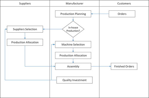
Figure 2 describes the flowchart of the system considered in this paper. After receiving an order from customers, the manufacturer includes the orders into the production planning. Afterwards, the manufacturer decides which components must be produced in-house and which components must be outsourced. After this decision, then the manufacturer needs to improve the quality of their components. The manufacturer provides some funds for both in-house process and suppliers process to improve the quality. Hence, the decision is about the investment allocation to the selected machine or supplier. The decision represents the second stage of optimization. After finishing the production process of each component, then the components must be assembled together into a final product and it is assumed that the assembly is performed after all components arrived in the assembly station. After all components have been assembled then the final product will be delivered to the customers.

Figure 2. The flowchart of decision process.

The framework of the models developed in this paper is depicted in Figure 3. From the figure, we can see that in the first stage, the manufacturer determines the optimal combination of components allocation using in-house/outsourcing production alternatives. The objective function of the model is to minimize manufacturing cost and quality loss. The outputs of the model are the amount of components allocation to each selected process/supplier and the variance of the components. The variance will be used as the input for the second stage. In the second stage, due to the regular production of the components, the company has a commitment to continuously improve the quality of the final product through process improvement in the components level. The quality of the components can be improved by reducing the variance of certain quality characteristics of the components. Hence, the components quality in term of components variance as the output of the first stage in the optimization framework must be improved in the second stage. The quality improvement of the components from both process/suppliers needs some investments in term of technology or human capital. The ROI will be used as the objective function of the second stage of optimization.

Figure 3. The optimization framework.

The notations used in this paper are as the following:

Table

i	Quality level index, i =  1,2,3,………I
j	Component index, m = 1,2,3…….J
k	Machine index, k = 1,2,3……..K
l	Supplier index, l = 1,2,3,………L
MCjk	Manufacturing cost of component j in machinek
PCjl	The price of component j by supplier l
bjk	Binary variable of component j in machine k
bjl	Binary variable of component j by supplier l
cjk	Production capacity of component j in machine k
cjl	Production capacity component j supplier l
Xjk	The amount of component j in machine k
Yjl	The amount of component j by supplier l
tjk	Tolerance of component j in machinek
tjl	Tolerance of component j from supplier l
TA	Assembly tolerance limit
Nj	The number of component j in final assembly
D	Demand of final assembly
Cp	Process capability index
TC	Total cost
f(y)	The density function of the probability distribution of quality characteristic y
${\sigma }_j^2$	Variance of component j
${\sigma }_A^2$	Variance of assembly
p	Planning periods
g(t)	The planning periods
ROI	Return on Investment
QL	Initial quality loss
QL*	Quality loss due to variance reduction
LC*	Optimal learning investment
A	Quality loss coefficient
λ*	Optimal learning rate
Ie	Coefficient for the exponential investment function
p	Proportion of variance reduction

3. Mathematical model formulation

3.1. Stage i model

Stage I model is developed to simultaneously determine the optimal tolerance of each component needed in assembly process through process/supplier selection and also the allocation of each component to the selected process/supplier. The objective function of the model is to minimize manufacturing cost and quality loss. The objective function of the model can be expressed as follows:

(1) $MinTC=\sum _{j=1}^J\left(\sum _{k=1}^K\left(M{C}_{jk}{X}_{jk}{b}_{jk}\right)+\sum _{l=1}^L\left(P{C}_{jl}{Y}_{jl}{b}_{jl}\right)\right)+\left(QL\right)$(1)

The first and second terms in Equation (1) represent the manufacturing cost and purchasing cost of all components needed in assembly process. The third term in the equation represents the Taguchi quality loss that quantify the loss of customers. The Taguchi quality loss is used in this model due to its simplicity and without loss of generality, other quality loss will also applicable in the model.

There are five constraints considered in the Stage I model: quality requirements in term of assembly tolerance limit, production capacity of in-house production and suppliers, minimum number of selected process/supplier, final product demand, and binary constraints.

(1) Assembly tolerance limit. This constraint is required to ensure the quality of the final product assembly. The sum of all component tolerances involved in assembly process should not exceed the assembly requirement. This constraint and the assembly variance are defined as follows:

(2) $\sum _{j=1}^J{\sigma }_j^2\le {\sigma }_A^2$(2)

(3) ${\sigma }_A^2={\left(\frac{T_A}{3Cp}\right)}^2$(3)

Since the component variances used in the assembly come from several sources with different values then we need a single value to represent the component variances. The single value of the variances can be calculated as follows:

(4) ${\sigma }_j^2=\frac{{\sum }_{k=1}^K{\left(\frac{T_{jk}}{3Cp}\right)}^2{X}_{jk}+{\sum }_{m=1}^M{\left(\frac{T_{jm}}{3Cp}\right)}^2{Y}_{jm}}{X_{jk}+Y_{jm}}\mathrm{\forall }j$(4)

(2) Production capacity. This constraint is needed to ensure that the amount of component allocations does not exceed the production capacities both in the case of in-house and outsource. The following equations expressed in-house and outsource capacities, respectively:

(5) $\sum _{k=1}^K{X}_{jk}{b}_{jk}\le c_{jk}$(5)

(6) $Y_{jm}{b}_{jm}\le c_{jm}$(6)

(3) Demand of final product. This constraint ensures that the each component needed in the assembly equals to the components needed in final assembly. Equation (7) expresses the constraint:

(7) $\sum _{k=1}^K{X}_{jk}{b}_{jk}+\sum _{m=1}^M{Y}_{jm}{b}_{jm}=n_{j}D$(7)

(4) Minimum number of selected process or supplier. This constraint is necessary to ensure that each needed component is available for the assembly process:

(8) $\sum _{k=1}^K{b}_{jk}+\sum _{m=1}^M{b}_{jm}$(8)

(5) Binary constraints. These constraints represent the selection process both for in-house production and outsource (1 if selected, 0 otherwise):

(9) $b_{jk}\in \left\{0,1\right\}\mathrm{\forall }j,$(9)

(10) $b_{jm}\in \left\{0,1\right\}\mathrm{\forall }j,k$(10)

3.2. Stage II model

The objective function of Stage II model is to maximize the ROI, in which the ROI is the common measure of investment effectiveness in project selection. The aim of the model is to determine optimal proportion value of variance reduction. Hence the company has to set the variance reduction target of a component and the target will be allocated to the selected process/suppliers. The variance reduction will have investment consequence. Hence, the manufacturer has to maximize the ROI to obtain optimal variance reduction. Three variables will affect the ROI, namely the initial quality loss, quality loss cost due to variance reduction, and total learning investment. Equation (11) expresses the quality loss function (manufacturers and suppliers) (Feng et al., 2001). Taguchi Loss function is used to quantify the quality loss which measure the loss of customer due to the bias and variance of a certain product quality characteristics. Since we assume that the nominal target value can be achieved by each process, then the quality loss will only depend on the variance of a certain product quality characteristic. In Equation (11) the right side of the equation has been defined in Equation (4):

(11) $Q_L=A\sum _{j=1}^J{\sigma }_j^2$(11)

Equations (12)-(18) are basically taken from Moskowitz et al. (2001). The second variable of ROI is shown in Equation (12). The equation expresses the quality loss after learning investment to get better quality product in term of lower quality loss:

(12) $Q_L^{\ast }=Q_L{\left(\frac{g\left(t\right)}{g\left(t\right)-1}\right)}^{-{\lambda }^{\ast }}$(12)

Equation (13) expresses the optimal learning rate. This equation is based on the exponential investment function in which the cost coefficient (I_e ) can be obtained by

(13) ${\lambda }^{\ast }=\frac{ln{Q}_L+\mathrm{l}\mathrm{n}\left(ln\left(\frac{g\left(t\right)}{g\left(t\right)-1}\right)\right)-ln{I}_e}{1+ln\left(\frac{g\left(t\right)}{g\left(t\right)-1}\right)}+0.5{\sigma }_{g\left(t\right)}^2\left(ln\left(\frac{g\left(t\right)}{g\left(t\right)-1}\right)-1\right)$(13)

(14) $I_e=L_{Cg\left(t\right)}{\left(e^{\lambda }-1\right)}^{-1}$(14)

In Equation (14), the learning rate (λ) can be obtained using Equation (15) and by inserting that value into Equation (16), we can determine the current learning investment:

(15) $\lambda =\frac{ln\left(p\right)}{ln\left(g\left(t\right)-2\right)-ln\left(g\left(t\right)-1\right)}$(15)

(16) $L_{Cg\left(t\right)}=L_{Cg\left(t\right)-1}\left(p\right){\left(\frac{g\left(t\right)}{g\left(t\right)-1}\right)}^{-\lambda }$(16)

Based on optimal learning rate in Equation (13) and the current learning investment in Equation (16) then the optimal learning investment is obtained by Equation (17). Finally, the optimal variance reduction resulted from such investment can be obtained as follows:

(17) $L_C^{\ast }=L_{Cg\left(t\right)}\left(e^{{\lambda }^{\ast }}-1\right)$(17)

(18) $\sigma { }_{g\left(t\right)}^2\ast ={\sigma }_{g\left(t\right)}^2{\left(\frac{g\left(t\right)}{g\left(t\right)-1}\right)}^{-{\lambda }^{\ast }}$(18)

Equations (19) and (21) are taken from Rosyidi, Nugroho, Jauhari, Suhardi, and Hamada (2016c). Equation (19) expresses the objective function of the model., while Equations (20) and (21) are the constraints imposed to the model:

(19) $MaxROI=\frac{A{\sum }_{j=1}^J{\sigma }_{jg\left(t-1\right)}^2-Q_L{\left(\frac{g\left(t\right)}{g\left(t\right)-1}\right)}^{-{\lambda }^{\ast }}}{L_{Cg\left(t\right)}\left(e^{{\lambda }^{\ast }}-1\right)}x100\mathrm{\%}$(19)

The first constraint in Equation (20) deals with the maximum available investment provided by the manufacturer to improve the component quality through learning. This constraint is needed to ensure that the total investment for component quality improvement from each selected process/supplier will not exceed the maximum investment provided by the manufacturer. The second constraint in Equation (21) deals with the optimal learning rate which must be better than the current learning rate.

(20) $\sum _{k=1}^K\sum _{l=1}^L{L}_{Cjkl}\le L_{Cj}^{max}$(20)

(21) ${\lambda }_j^{\ast }\ge {\lambda }_j$(21)

4. Numerical example and analysis

4.1. Numerical example

A numerical example is given to show the applicability of the model. We use the case of assembly in Cao, Mao, Ching, and Yang (2009) due to its simplicity in which the dimensional chain of the assembly is shown in Figure 4. The assembly consists of three components: Revolution axis, End shied nut, and Sleeve. The quality characteristic of each component was denoted by x₁, x₂ , and x₃ and assumed to be normally distributed with the mean of µ₁  = 38.00 mm, µ₂  = 42.00 mm, and µ₃  = 80.00 mm, respectively. The quality characteristic of the product is x₀ in which the dimension must be less than 0.02 mm to make the product well functioned. Manufacturing cost and supplier component prices are shown in Tables 1, 2 and 3. The tables also show the tolerance for each alternative. In-house production and the suppliers have the same opportunity to fulfil the demand of the components.

Table 1. Component characteristics at each machine of Cell 1

	Machine 1			Machine 2			Machine 3
Component	Tol. (mm)	Cost (IDR)	Proc.Time (min/unit)	Tol. (mm)	Cost (IDR)	Proc.Time (min/unit)	Tol. (mm)	Cost (IDR)	Proc.Time (min/unit)
1	0.008	8,000	9	0.005	10,000	14	0.003	12,000	13
2	0.008	9,000	10	0.005	11,500	15	0.003	13,000	14
3	0.008	12,000	12	0.005	13,000	18	0.003	15,000	16

Table 2. Component characteristics at each machine of Cell 2

	Machine 1			Machine 2			Machine 3
Component	Tol. (mm)	Cost (IDR)	Proc.Time (min/unit)	Tol. (mm)	Cost (IDR)	Proc.Time (min/unit)	Tol. (mm)	Cost (IDR)	Proc.Time (min/unit)
1	0.006	11,000	12	0.0045	12,000	9	0.007	8,000	15
2	0.006	13,500	14	0.0045	14,000	9	0.007	8,500	16
3	0.006	15,000	17	0.0045	16,000	10	0.007	15,000	18

Table 3. Component characteristics from suppliers

Component	Supplier 1			Supplier 2
	Tol. (mm)	Cost (IDR)	Proc.Time (min/unit)	Tol. (mm)	Cost (IDR)	Proc.Time (min/unit)
1	0.0095	18,000	25	0.015	20,000	20
2	0.0095	20,000	32	0.015	21,000	24
3	0.0095	22,500	35	0.015	23,500	31

Figure 4. Dimensional chain of the assembly product (Adapted from Cao et al., 2009 ).

The company received an order of 300 units of final product. The capacity of each Machine and Supplier are shown in Table 3. We assume the component routings consist of two stages as shown in Table 4. The manufacturer has two cells to manufacture the components in which each cell consists of three machines of the same types. In the numerical example, it is assumed that all machines have the same process capability indices of C_p = 1 for each component. The cost coefficient of the quality loss is assumed to be IDR 1,000,000.

Table 4. Routing of Each Component for in-house production

Component	Stage 1	Stage 2
1	Cell 1	Cell 2
2	Cell 2	Cell 1
3	Cell 1	Cell 2

OptQuest of Oracle Crystal Ball software is used to solve the numerical example. OptQuest will perform the searching process until it finally reaches some termination criteria, either a maximum number of iterations or a limit on the amount of time devoted to the search. The results show that the optimal decision from the model in this numerical example is mixed between in-house production and outsourcing as shown in Table 5. From Table 5, we can see that 36.67% of Component 1 are produced in-house while 63.33% of them are outsourced. For this component, the model found the big portion of components quantity came from the machines with the lowest cost (33.33%) and supplier with lowest price (40%). Component 2 gives different results. The majority allocations of this component came from the machine with tight tolerance (33.33%) and supplier with the lowest price (25%). Component 3 has the same pattern with Component 2 in term of quantity allocation. Table 6 shows the breakdown of the total cost. From the table, we can see that manufacturing and purchasing costs comprise about 95% of the total cost.

Table 5. The optimization results of Stage 1 Model

	Stage 1			Stage 2
Component	M 1	M 2	M 3	M 1	M 2	M 3	Supplier 1	Supplier2
1	105	5	0	100	10	0	120	70
2	5	130	85	15	100	105	75	5
3	0	65	115	85	0	95	105	15

Table 6. The breakdown of costs component

Component of Cost	Amount
Manufacturing Cost	IDR. 6,825,001
Purchasing Cost	IDR. 7,880,000
Lateness Cost	IDR. 423,750
Quality Loss Cost	IDR. 147,942
Total Cost	IDR. 15,276,693

From the optimization results of Stage 1 Model, the Stage 2 Model is then solved using the same software. The optimal variance reduction before and after learning investments are shown in Table 7. The table shows significant quality improvement in term of variance reduction. The average improvements for both in-house production and outsource are 28.11% and 41.82%, respectively.

Table 7. The optimization results of stage 2 model

	In-House Production		Outsource
Component	Before	After	Before	After
1	0.0011830	0.0007062	0,0012076	0.0007891
2	0.0007678	0.0006097	0,0007523	0.0003771
3	0.0006366	0.0004874	0,0010537	0.0006222

The optimal allocations of learning investment are listed in Table 8. From the table, the optimal learning investment allocation for Component 1, 2, and 3 are IDR. 7,674,896, IDR. 6,380,308, and IDR. 5,984,813, respectively, with total investment of IDR. 20,040,017. The ROI resulted from the Stage 2 Model are 53%, 69%, and 72% for Component 1, 2, and 3, respectively,

Table 8. The optimal investment allocations from Stage 2 Model

	Learning Investment
Component	In-House Production	Outsource	Total
1	IDR. 4,282,204	IDR. 3,392,692	IDR. 7,674,896
2	IDR. 2,125,595	IDR. 4,254,712	IDR. 6,380,308
3	IDR. 2,355,672	IDR. 3,629,140	IDR. 5,984,813
TOTAL			IDR. 20,040,017

4.2. Sensitivity analysis

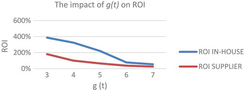
To gain further insights into the behaviour of the model, we examine the effect of the changes in some important parameters to the optimal solutions. The increase of $g\left(t\right)$ will increase the learning investment and decrease the quality loss, which will result in the decrease of total ROI. Table 9 shows the results of the sensitivity analysis of the changes of g(t) on the ROI while the representation graph of the table is shown in Figure 5. From Table 9, the increase of g(t) will decrease of ROI due to the longer time of the periods. The ROI of in-house production in average is more than twice higher than the outsource production for all periods. It indicates that the investment of the quality improvement in their own production processes is more effective than in the suppliers side. Since the investment came from the manufacturer, then both investments give benefits to the manufacturer in reducing the quality loss.

Table 9. Results of the change of g(t) to the ROI

	In-House				Supplier
(t)	Comp.1	Comp. 2	Comp. 3	Average ROI	Comp. 1	Comp. 2	Comp. 3	Average ROI
3	152%	314%	695%	387%	270%	64%	209%	181%
4	72%	321%	579%	324%	99%	49%	152%	100%
5	56%	201%	406%	221%	82%	35%	79%	65%
6	42%	94%	98%	78%	47%	23%	42%	37%
7	42%	66%	54%	54%	37%	13%	29%	26%

Figure 5. The impact of learning period on ROI.

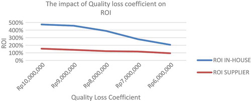
The increase of quality cost coefficient will not directly affect the increase of learning investment. It will affect the decrease of total quality loss and eventually will decrease the total ROI. The impact of quality cost coefficients on the ROI are shown in Table 10, while the graphical representation of the table is shown in Figure 6. In average, the increase of quality cost coefficient will increase the ROI both in-house production and outsource production. This results came from the fact that the higher the quality coefficient, the higher the difference between quality loss before and after quality improvement.

Table 10. The impact of quality coefficient on the ROI

	In-House				Supplier
Quality Cost Coefficient	Comp. 1	Comp. 2	Comp. 3	Average ROI	Comp. 1	Comp. 2	Comp. 3	Average ROI
10,000,000	93%	749%	583%	475%	203%	148%	112%	155%
9,000,000	138%	227%	1011%	458%	114%	81%	223%	139%
8,000,000	108%	916%	147%	390%	114%	113%	140%	122%
7,000,000	74%	564%	203%	280%	169%	72%	109%	117%
6,000,000	84%	209%	325%	206%	100%	74%	111%	95%

Figure 6. The impact of quality loss coefficient on ROI.

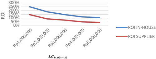
The increase of $L{C}_{kg\left(t-1\right)}$ will increase the learning investment, decrease the quality loss, and eventually will result in the decrease of the ROI. In average, the increase of $L{C}_{kg\left(t-1\right)}$ will decrease the ROI both in-house production outsource production. The change of $A$ gives fair significant impact to the objective function and decision variables compare to the other parameters. The results of sensitivity analysis of this parameter are shown in Table 11 while the graphical representation of the table is shown in Figure 7.

Table 11. The impact of $L{C}_{kg\left(t-1\right)}$ on the ROI

$\mathit{L}{C}_{kg\left(t-1\right)}$	In-House			Average ROI	Supplier			Average ROI
	Comp.1	Comp.2	Comp.3		Comp.1	Comp.2	Comp.3
1,000,000	93%	749%	583%	475%	127%	178%	136%	147%
2,000,000	138%	227%	1011%	458%	134%	55%	82%	91%
3,000,000	108%	916%	147%	390%	132%	29%	65%	75%
4,000,000	74%	564%	203%	280%	70%	33%	53%	52%
5,000,000	84%	209%	325%	206%	69%	23%	41%	44%

Figure 7. The impact of $\mathit{L}{C}_{kg\left(t-1\right)}$ on the ROI.

5. Conclusions

In this paper, a two-stage optimization model for process/supplier selection, component allocation and quality improvement has been developed. The Stage 1 of the model dealt with simultaneous determination of optimal components tolerance through process/supplier selection and components allocation to the selected process/supplier. The objective function of the first stage model was to minimize manufacturing cost and quality loss. Stage 2 model dealt with quality improvement through optimal allocation of learning investment to the selected process/supplier. The objective function of the model was to maximize the ROI as a common effective measure of investments. The quality improvement was made through variance reduction of components both at manufacturer and supplier sides. From the sensitivity analysis, we found that periods of investment, quality cost coefficient, and $L{C}_{kg\left(t-1\right)}$ will affect the ROI. The latter parameter has the most significant effect on the ROI compared to the first two parameters. Hence the manufacturer has to set the current learning investment more precise than the other parameters. In future research, this model can be expanded by incorporating the uncertainty both in the quality loss and learning cost investment function. Hence, fuzzy quality loss and some probability distributions can be involved in the model. Another future research can be performed by integrating the model with lotting size decisions and production scheduling.

Additional information

Funding

The authors received no direct funding for this research.

Notes on contributors

Cucuk Nur Rosyidi

Cucuk Nur Rosyidi is a lecturer in Master Program of Industrial Engineering at Universitas Sebelas Maret. His doctoral degree was obtained from Institut Teknologi Bandung Indonesia in the field of Manufacturing Systems in 2010. He currently serves as the Chief of Center for Research in Manufacturing Systems (CRiMS). His research interests include product design and development, quality engineering, and system modeling.

Mega Aria Pratama

Mega Aria Pratama is the alumni of Industrial Engineering of Universitas Sebelas Maret both for undergraduate and master program. He graduated from the master program on February 2018. His research interests include production system, mathematical modeling, and simulation. He currently works as a project manager in PT. Harmony Land Group to control sales and marketing performance, construction performance and cash flow of the company.

References

- Adler, P. A. , & Clark, K. B. (1991). Behind the learning curve: A sketch of the learning process. Management Science , 37(3), 267–281. doi:10.1287/mnsc.37.3.267
- Barthelemy, J. & Adsit, D. (2003). The seven deadly sins of outsourcing. Academy of Management Executive , 17(2), 87–100.
- Bernstein, F. , & Kok, A. G. (2009). Dynamic cost reduction through process improvement in assembly networks. Management Science , 55(4), 552–567. doi:10.1287/mnsc.1080.0961
- Cao, Y. , Mao, J. , Ching, H. , & Yang, J. (2009). A robust tolerance optimization method based on fuzzy quality loss. Proceedings of the Institution of Mechanical Engineers, Part C: Journal of Mechanical Engineering Science , 223, 2647–2653. doi:10.1243/09544062JMES1451
- Chase, K. W. , Greenwood, W. H. , Loosli, B. G. , & Hauglund, L. F. (1990). Least cost tolerance allocation for mechanical assemblies with automated process selection. Manufacturing Review , 3(1), 49–59.
- Chen, J.-M. , & Tsou, J.-C. (2003). An optimal design for process quality improvement: Modelling and application. Production Planing and Control , 14(7), 603–612. doi:10.1080/09537280310001626197
- Feng, C.-X. , Wang, J. , & Wang, J.-S. (2001). An optimization model for concurrent selection of tolerance and suppliers. Computers & Industrial Engineering , 40(1–2), 15–33. doi:10.1016/S0360-8352(00)00047-4
- Fors, H. N. , Harraz, N. A. , & Abouli, M. G. (2011). Supplier selection and order allocation in supply chain management. Proceedings of the 41st international conference on computers & industrial engineering . Los Angeles California USA, 23-25 October 2011, 116–121. doi: 10.1177/1753193410382720
- Ganeshan, R. , Kulkarni, S. , & Boone, T. (2001). Production economics and process quality: A Taguchi perspective. International Journal of Production Economics , 7, 343–350. doi:10.1016/S0925-5273(00)00130-4
- Ghorbeni, M. , Bahrami, M. , & Arabzad, S. M. (2012). Integrated model for supplier selection and order allocation; using Shannon enthropy, SWOT, and linear programming. Procedia Social and Behavioral Sciences , 14, 521–527. doi:10.1016/j.sbspro.2012.04.064
- Lapre, M. A. , Mukherjee, A. S. , & Van Wassenhove, L. N. (2000). Behind the Learning Curve: Linking Learning Activities to Waste Reduction. Management Science , 46, 597–611. doi:10.1287/mnsc.46.5.597.12049
- Moskowitz, H. , Plante, R. , & Tang, J. (2001). Allocation of quality improvement target based on investments in learning. Naval Research Logistics , 48, 684–709. doi:10.1002/nav.1042
- Plante, R. (2000). Allocation of variance reduction targets under the influence of supplier interaction. International Journal of Production Research , 38(12), 2815–2827. doi:10.1080/002075400411493
- Pratama, M. A. , & Rosyidi, C. N. (2017, December 6–8). Make or buy decision model with multi-stage manufacturing process and supplier imperfect quality . AIP conference proceedings of International Materials, Industrial and Manufacturing Engineering Conference, MIMEC 2017. Miri, Malaysia. 020026-1-020026-10. doi:10.1063/1.5010643
- Rosyidi, C. N. , Jauhari, W. A. , Suhardi, B. , & Hamada, K. (2016b). A variation reduction allocation model for quality improvement to minimize investment and quality costs by considering suppliers’ learning curve. IOP Conference Series: Materials Science and Engineering , 114, 1–5. doi:10.1088/1757-899x/114/1/012083
- Rosyidi, C. N. , Murtisari, R. , & Jauhari, W. A. (2016a). A concurrent optimization model for suppliers selection, tolerance and component allocation with fuzzy quality loss. Cogent Engineering , 3, 1. doi:10.1080/23311916.2016.1222043
- Rosyidi, C. N. , Murtisari, R. , & Jauhari, W. A. (2017). A concurrent optimization model for supplier selection with fuzzy quality loss. Journal of Industrial Engineering and Management , 10(1), 98–110. doi:10.3926/jiem.800
- Rosyidi, C. N. , Nugroho, A. W. , Jauhari, W. A. , Suhardi, B. , & Hamada, K. (2016c). Quality improvement by variance reduction of component using learning investment allocation model. International conference on industrial engineering and engineering management, IEEM 2016 , Bali, Indonesia , 4–7 December 2016. 391–394. doi:10.1109/IEEM.2016.7797903
- Tsou, J.-C. , & Chen, J.-M. (2005). Case study: Quality improvement model in a car seat assembly line. Production Planning & Control: The Management of Operations , 16(7), 681–690. doi:10.1080/09537280500249223