On the prediction capabilities of two SGS models for large-eddy simulations of turbulent incompressible wall-bounded flows in OpenFOAM

Abstract

A comprehensive evaluation of the prediction capabilities of two Sub-Grid-Scale (SGS) models, for Large-Eddy Simulations (LES) of incompressible turbulent flows, is performed by studying two cases of flows through wall-bounded domains: a standard smooth-wall channel and a channel featuring fixed geometrical perturbations in its bottom wall. The SGS models were computationally implemented in OpenFOAM’s framework and numerical results have been evaluated using available DNS data of turbulent flow in the standard channel flow case at four different friction Reynolds numbers, i.e. Reτ =180, 395, 550 and 950. A number of well-known features were employed to judge about the reliability of the selected SGS models in the standard channel case, including: mean flow velocity profiles, ensemble averages of first and second-order turbulent statistics, and profiles of TKE. One of the SGS models was employed to explore the second case, a flow with high levels of strain and formation of large-scale vortical structures induced by cavities and/or ribs-like protuberances in one of the boundaries. Our numerical experiments show that both SGS models exhibit good quantitative and qualitatively agreement with most of the important flow features in both wall-bounded flows considered, although the attained levels of accuracy exhibited a mesh-resolution dependency. In the non-smooth-wall case, the selected SGS model was able to successfully capture, in accurate manner, effects as turbulence modulation and changes of the skin friction coefficient. It is clear that the implementations of the SGS models were successful in predicting the turbulent behaviour of the selected flow cases.

Keywords:

• turbulence
• large-eddy simulations
• sub-grid scale models
• OpenFOAM

PUBLIC INTEREST STATEMENT

In this manuscript, we report and analyse the results of a complete assessment of the prediction capabilities of two in-house implementations of Sub-Grid-Scale-based (SGS) models for use in simulation of turbulent incompressible flows by the Large-Eddy-Simulation (LES) method using the software OpenFOAM. We focused our attention on the Dynamic Smagorinsky and the Coherent Structures' SGS-models. Although these models have shown to have high levels of accuracy for predicting turbulence dynamics on several applications, there is not an official implementation and validation of their performance in the open-source software OpenFOAM, now widely used by many researchers and companies. Our results showed that both implementations were able to capture the turbulent dynamics of a plane channel flow for different Reynolds numbers with adequate levels of accuracy to effectively assess incompressible turbulent flows.

1. Introduction

Turbulence in fluid transport processes is a phenomenon that involves fluid motions at a large range of physical scales, and hence commonly associated with a broad range of spatial and temporal characteristics. In general, the largest spatial scales are mainly determined by the geometry involved in a given case, whereas the smaller ones are usually dominated by the flow regime, and therefore characterised with Reynolds numbers. For instance, as the Reynolds number is increased, the size of the characteristic lengths used to define the small-scale range becomes even smaller (Moeng & Sullivan, 2015). This coexistence of multiple physical features produces a highly dynamical behaviour in turbulent flows. In computational fluid dynamics, there are different strategies to tackle turbulence and its rich dynamical behaviour. Each of these strategies presents different degrees of reliability, accuracy, applicability, and success. The most accurate of them is Direct Numerical Simulations (DNS), where the computational model aims to explicitly resolve all relevant physical scales; nevertheless, this level of accuracy and resolution usually implies an extremely high, sometimes even prohibitive, computational cost. This feature of DNS is usually regarded as a constraint, difficult to overcome, especially when access to high-performance computing facilities is not readily available. Precisely, such a pitfall has driven the search for alternative strategies with lower computational requirements, but in line with the level of complexity of the flow and the degree of accuracy required by a specific application (Girimaji & Abdol-Hamid, 2005).

One of the alternative strategies to DNS turbulence modelling is the well-known Large-Eddy Simulations approach, also known as LES modelling. Under the LES approach the largest eddies, which contain most of the turbulent kinetic energy (TKE) associated with the main flow, are explicitly resolved while the smaller eddies are modelled.

These smaller scale eddies are commonly known as sub-grid scale (SGS) eddies. LES relies on the assumption that the large-scale flow structures carry most of the energy, and those associated to smaller scales have mainly a physical dissipative effect (Sagaut, 2006); however, one important thing to be noted is that the level of accuracy in the computation of the largest scales is influenced by the accuracy of the modelling of the smallest scales (John, 2012). Since not all the scales are explicitly resolved, LES approach has proved to require lesser computational effort than DNS simulations. (Marchioli, 2017; Piomelli, 2014; Zhiyin, 2015). In any case, as LES relies upon the distinction between large and small scales, it is essential to define a threshold to distinguish between large- and small-scale eddies. This threshold is usually defined by the flow condition, although the available computational power or numerical method very often determine the set of scales to be effectively computed. As a spatial discretization is usually unavoidable in the majority of computational fluid dynamics applications, it is very common to implicitly use the size of the computational mesh as a mechanism to define the required threshold. This way to distinguish between scales to be modelled and scales to be fully resolved is usually named as implicit filtering. When implicit filtering is used, the spatial grid largely dictates the scales that can be fully resolved by the numerical model. Hence, it is clear that in LES the mesh width or grid size is a restriction on the size of the eddies that are to be modelled explicitly, i.e. eddies smaller in length than a particular grid size. Any other eddy will have to be included in the set of structures that should be modelled. This particular set of structures constitutes the so-called small-scale or sub-grid-scale eddies (SGS eddies). In order to model such SGS eddies a number of different kinds of SGS modelling methods have been developed. Most of them involve an eddy-viscosity assumption based on the Boussinesq’s hypothesis (Kajishima & Nomachi, 2006; Lesieur & Metais, 1996; Veloudis, Yang, & McGuirk, 2008). Furthermore, the most commonly used SGS models are variants of the standard Smagorinsky model (SM) (Smagorinsky, 1963), all which present as main advantage the ability to properly represent the process of transfer of kinetic energy from the largest scales to the smaller ones until this energy is dissipated through viscous effects. Nevertheless, these kinds of models have several limitations including poor correlation coefficients (Bardino, Ferziger, & Reynolds, 1983; Clark, Ferziger, & Reynolds, 1979), as well as the inability to capture the back-scattering effect from the smallest eddies to larger eddies (Dubois & Bouchon, 1998). One variant of such SGS models is the Dynamic Smagorinsky (DS) model proposed by (Germano, Piomelli, Moin, & Cabot, 1991) and modified by (Lilly, 1992), which aims to subdue some of the shortcomings of the original SM model. The DS model is currently one of the most widely used in production simulations and its arguably high level of acceptance can be explained by the high level of good agreement between its numerical predictions and the experimental and DNS data available (Dritselis & Vlachos, 2011a, Mallouppas & van Wachem, 2013; Pantano, Pullin, Dimotakis, & Matheou, 2008).

However, the DS model also exhibits some difficulties: (i) as the model parameter is locally determined, it could produce large negative values for long periods of time and over large regions, eventually leading to numerical instabilities; (ii) the parameter variation can be too large, which might result in a variance of about 10 times the mean if not properly addressed; (iii) the DS model needs more computational effort, at least in comparison with the standard Smagorinsky model, due to the need for locally computing the Smagorinsky coefficient. The first two disadvantages have commonly been addressed by using a procedure proposed by (Lilly, 1992) where the model parameter is computed by an average process in homogeneous directions, so avoiding possible negative values and reducing the variance of the modelling parameter.

For practical purposes it is desirable to use SGS models that demand lesser computational resources compared to the DS model but with similar levels of accuracy. According to this, different SGS models have been developed and proposed, as in (Inagaki, Kondoh, & Nagano, 2005, Vreman, 2004; Yoshizawa, Kobayashi, Kobayashi, & Taniguchi, 2000). These models have in common that the turbulent eddy-viscosity is locally determined using fixed model-parameters. These models have already shown better performance than the SM model for turbulent channel flows, as reported in (Inagaki et al., 2005) and (Vreman, 2004) and discussed by (Kobayashi, Ham, & Wu, 2008). Precisely, another SGS model that has been proposed is the Coherent Structures model (CS) presented in (Kobayashi, 2005), which has shown to produce very accurate results with lower computational costs compared to the DS model (Dritselis, 2014).

The CS model is an SGS model based on the behaviour of the coherent structures extracted using the ”Q” invariant, as defined by (Hunt, Wray, & Moin, 1988). This SGS model relies on the fact that the Q-coherent structures have a direct relationship with the estimated amount of energy dissipation by the SGS eddies (Kobayashi, 2005).

Even though both SGS models, the Dynamic Smagorinsky and Coherent Structures models, have been present in the research community for quite some time, not many commercial or open-source CFD codes have officially implemented or made readily available such SGS models. For instance, although OpenFOAM (an open-source CFD computational framework) officially supports different Sub-Grid Scale (SGS) models for Large-Eddy Simulations including the Standard Smagorinsky, WALE, and one-equation Eddy, among others, it lacks official implementations of the DS and CS models. Nevertheless, thanks to its open-source nature, a version of the DS model has been made available by the OpenFOAM community (see 2010–2014 Alberto Passalacqua). In any case, despite of being used in different CFD projects, there are not assessments and/or validation studies for such a Dynamic Smagorinsky SGS model under OF framework yet published or available. In the case of the Coherent Structures model situation is similar: there are not yet known official or unofficial implementations in OpenFOAM (OF), and therefore there is a lack of information available about its reliability and performance when used within this open-source platform.

The numerical experiments of the present work have been focused on exploring the aforementioned SGS models in OpenFOAM. The interest of the present work in OpenFOAM as computational simulation framework for CFD projects is twofold: first, since its introduction into the academic world, OpenFOAM (OF) has constantly attracted the attention of multiple research groups and academic institutions, making it one of the most commonly computational tools amongst many research groups; secondly, OpenFOAM (OF) provides a computational framework that can be modified by users to suit many different applications related to continuum fluid mechanics, allowing relatively fast development and implementation of many physics models and solvers. In fact, one of the many features that has constantly driven many researchers to use OpenFOAM as simulation tool is the possibility to quickly modify and adapt its source code, and then enabling to perform numerical simulations in a wide range of applications such as atmospheric boundary layer modelling for wind turbine studies, turbulence, combustion, turbo machinery among many others (De Villiers, 2007; Doolan, 2009; Flores, Garreaud, & Mun˜oz, 2014; Higuera, Lara, & Losada, 2014; Jacobsen, Fuhrman, & Fredsøe, 2012; Lysenko, Ertesv°ag, & Rian, 2013; Peltola et al., 2011; Robertson, Choudhury, Bhushan, & Walters, 2015).

Nevertheless, in spite of its many attractive features, OF has some disadvantages as well. The most important one is the reduced number of published validation tests for the majority of physical models already implemented. In any case, due to the increasing impact of OF on research and industrial projects, in recent years several studies have focused on validating some of the OF numerical implementations, as those reported in (Churchfield, Sang, & Moriarty, 2013; De Villiers, 2006; Doolan, 2009; Muntean, Nilsson, & Susan-Resiga, 2009; Nilsson, 2007; Panjwani et al., 2014). One of the most complete studies in turbulence modelling using OF was published by (Lysenko et al., 2013), where turbulent separated flows over circular and triangular cylinders in a channel were used to explore the compressible κ E model. This study also explored the OF parallel scalability, showing that the parallel performance of OF is good up to 1024 cores and providing results in agreement with experimental data and other numerical solutions. Also, Lysenko, Ertesv°ag, & Rian, (2012) studied some of the LES models available in OF for a flow over a circular cylinder, concluding that OF numerical methods are sufficiently accurate for LES calculations.

Accordingly, the main objective of the present work is threefold: firstly, to validate and asses the performance of the DS model implemented by the OF community, especially when employed for LES simulations of wall-bounded channel flows; secondly, to validate and asses an in-house implementation of the CS model under OF framework for simulation of turbulent wall-bounded flows; finally, a third objective of this work was to critically assess the prediction capabilities of the CS-SGS model in cases where high rates of shear stress are observed. Two different geometrical configurations were employed: a smooth-wall-bounded turbulent channel, where flow was simulated at four different friction Reynolds numbers, namely Re_τ = 180, 365, 550 and 950, and a channel featuring ribs-like protuberances and cavity-like perturbations in its bottom wall. This kind of geometric perturbations has been already used for other authors to evaluate turbulence modulation, skin friction coefficient changes and improvement of heat transfer rates through simple non-smooth walls (Leonardi, Orlandi, Smalley, Djenidi, & Antonia, 2003, Nagano, Hattori, & Houra, 2004; Orlandi, Leonardi, & Antonia, 2006).

Performance and prediction capabilities of the SGS models considered in this work were evaluated examining a number of turbulent channel flow features, mainly: mean velocity profiles, turbulence statistics in the near-wall region, and turbulent production and viscous dissipation of the kinetic energy budget. All results obtained with both SGS models are compared against DNS and LES data published by other authors. It is shown that both SGS-models predict similarly the turbulent dynamics of the flow, both being capable to accurately predict turbulent statistics of first and second order with a relatively low computational requirement.

In the non-smooth-wall cases, the geometrical perturbations were chosen to be in line with studies focused on turbulence modulation, such as those presented by (Chamorro, Arndt, & Sotiropoulos, 2013, El-Samni, Chun, & Yoon, 2007; Garc´ıa-Mayoral & Jim´enez, 2011; Jiménez, Wray, Saffman, & Rogallo, 1993; Leonardi, Orlandi, & Antonia, 2007; Nadeem, Lee, Lee, & Sung, 2015), among others. Equally, as in the DS case used in the smooth-wall channel flow, the numerical results show that our implementation of the CS-SGS model properly captures the first and second-order turbulent statistics, as well as other flow features previously reported by other researchers.

The present work has been structured as follows: the relevant mathematical model is presented in the next section, whereas details of the computational model are discussed in section three. The main body of numerical results is presented in section four with emphasis on mean velocity profiles, velocity fluctuations, and wall-normal profiles of turbulent production and viscous dissipation. Discussion about the level of accuracy obtained in predicting each of these flow characteristics in the smooth-wall channel flow, is also presented in this section. Next, results obtained with the CS SGS-model for channels with ribs-like protuberances and cavity-like perturbations on the bottom wall, as well as an assessment of its performance compared to DNS data available in literature, is presented in the next to last section. Finally, in the last section, we present some discussion and conclusions relevant to this and future work.

2. Background of LES method

2.1. Governing equations for LES approach

The Sub-Grid-Scale models considered in this paper are relevant to incompressible turbulent flows under conditions where the continuum assumption is valid.

Accordingly, the basic incompressible Navier-Stokes equations are an entirely valid starting mathematical model. However, as the main focus of this paper concerns Large-Eddy Simulations (LES), it is necessary to do a filtering process of the Navier-Stokes equations, producing a modified filtered version of these equations. For instance, some filtering techniques have been developed by different authors (Germano et al., 1991; Kobayashi, 2005; Smagorinsky, 1963) and are currently part of the mainstream LES codes, as presented by (Sagaut, 2006). The equations produced after the filtering procedure have a very similar mathematical form compared to the original Navier-Stokes equations, except for one additional term, which describes the behaviour of the so-called sub-grid scale stress tensor (τ_ij).

Once the filtering procedure is applied, the filtered Navier-Stokes equations can be written as

(1) $\frac{\mathrm{\partial }\overline{u_i}}{\mathrm{\partial }{x}_i}=0$(1)

(2) $\frac{\mathrm{\partial }\overline{u_i}}{\mathrm{\partial }t}+\frac{\mathrm{\partial }\left(\overline{u_i}\right)\left(\overline{u_j}\right)}{\mathrm{\partial }{x}_j}=-\frac{1}{\rho }\frac{\mathrm{\partial }\bar{p}}{\mathrm{\partial }{x}_i}+\nu \frac{{\mathrm{\partial }}^2\overline{u_i}}{\mathrm{\partial }{x}_j^2}-\frac{\mathrm{\partial }{\tau }_{ij}^R}{\mathrm{\partial }{x}_i}+{\mathrm{\Pi }}_i{\delta }_{i1}$(2)

where u_i is the component of the filtered fluid velocity in the i-th direction, p is the fluid pressure, and ρ and ν are the density and the kinematic viscosity of the fluid, respectively. ”Π” is an extra moment source term which represents the body forces acting over the flow, and in the present work is employed to keep the mass flow rate constant on each simulation. Finally, δ_ij is the Kronecker delta and ${\tau }_{ij}^R$ is the residual stresses tensor, defined as

(3) ${\tau }_{ij}^R=\overline{u_i{u}_j}-\left(\overline{u_i}\right)\left(\overline{u_j}\right)$(3)

As with any tensor, the residual stress tensor can be separated into its spherical and deviatoric components, and therefore be written as

(4) ${\tau }_{ij}^R={\tau }_{ij}^r+\frac{2}{3}{k}_R{\delta }_{ij}$(4)

where k_R is called the residual kinetic energy, and defined as

(5) $k_R=\frac{1}{2}{\tau }_{ii}^R$(5)

The spherical part of the residual stress tensor as well as the “Π” term, can be grouped with the pressure field term, which produces a new modified equivalent pressure field in the filtered Navier-Stokes equations, as shown in Equations 6(6) $\frac{\mathrm{\partial }\overline{u_i}}{\mathrm{\partial }t}+\frac{\mathrm{\partial }\left(\overline{u_i}\right)\left(\overline{u_j}\right)}{\mathrm{\partial }{x}_j}=\frac{\mathrm{\partial }\overline{p^{\ast }}}{\mathrm{\partial }{x}_i}+\nu \frac{{\mathrm{\partial }}^2\overline{u_i}}{\mathrm{\partial }{x}_j^2}-\frac{\mathrm{\partial }{\tau }_{ji}^r}{\mathrm{\partial }{x}_i}$(6) .

(6) $\frac{\mathrm{\partial }\overline{u_i}}{\mathrm{\partial }t}+\frac{\mathrm{\partial }\left(\overline{u_i}\right)\left(\overline{u_j}\right)}{\mathrm{\partial }{x}_j}=\frac{\mathrm{\partial }\overline{p^{\ast }}}{\mathrm{\partial }{x}_i}+\nu \frac{{\mathrm{\partial }}^2\overline{u_i}}{\mathrm{\partial }{x}_j^2}-\frac{\mathrm{\partial }{\tau }_{ji}^r}{\mathrm{\partial }{x}_i}$(6)

where

(7) $\frac{\mathrm{\partial }\overline{p^{\ast }}}{\mathrm{\partial }{x}_i}=-\frac{1}{\rho }\frac{\mathrm{\partial }\bar{p}}{\mathrm{\partial }{x}_i}-\frac{2}{3}\frac{\mathrm{\partial }{k}_R}{\mathrm{\partial }{x}_i}+{\mathrm{\Pi }}_i{\delta }_{i1}$(7)

As usually occurs with Reynolds-like decomposition, i.e. into an ”average” or filtered value plus a fluctuating value, the resulting flow governing equations conform an incomplete system of equations as the number of unknowns is increased. In this case, any additional expression, or system of expressions used to close the uncompleted filtered mathematical model is called an”SGS” model.

2.2. Sub-grid scale (SGS) models

As discussed briefly in the previous sections, the main component of a Large-Eddy Simulation is the mathematical construction used to model the sub-grid-scale (SGS) stresses, i.e. the deviatoric part of the residual stress tensor. Many different SGS models have been proposed but in the present work, only two of those SGS models have been explored, namely the Dynamic Smagorinsky model proposed by (Germano et al., 1991) and the more recent Coherent Structures model proposed by (Kobayashi, 2005). A short discussion on some of the details of these two models is presented next.

2.2.1. Dynamic smagorinsky model

Despite the relative small computational cost associated to the use of the Standard Smagorinsky model (Smagorinsky, 1963), such a model presents some problems in terms of its prediction capabilities, which usually cannot be improved with a simple mesh refinement. For example, in some complex turbulent flows, the constant of the standard Smagorinsky model lacks the essential universality character needed to model turbulent flows. Also, this model does not take into account the well-known energy back-scatter phenomenon (i.e., the energy flow from small scales to large scales) which in some flows is essential. For this reason, Germano et al. (1991) proposed a procedure to calculate the Smagorinsky constant as a function of space and time by assuming similarity of the filtered structures and applying a second filter to the filtered Navier-Stokes equations. This second filter is coarser than the original one used in the primary filtering process of LES simulations, and is commonly named as “test filter” ($\hat{\mathrm{\Delta }}>\mathrm{\Delta }$), where Δ is the original LES filter and $\hat{\mathrm{\Delta }}$ is the “Test filter”. After applying the test filter, a new filtered residual stress tensor is formed:

(8) $T_{ij}^R=\widehat{\stackrel{‾}{u_i{u}_j}}-\left(\widehat{\stackrel{‾}{u_i}}\right)\left(\widehat{\stackrel{‾}{u_j}}\right)$(8)

From Equations 8(8) $T_{ij}^R=\widehat{\stackrel{‾}{u_i{u}_j}}-\left(\widehat{\stackrel{‾}{u_i}}\right)\left(\widehat{\stackrel{‾}{u_j}}\right)$(8) and 4(4) ${\tau }_{ij}^R={\tau }_{ij}^r+\frac{2}{3}{k}_R{\delta }_{ij}$(4) , (Germano et al., 1991)(14) $Q=\frac{1}{2}\left(\overline{{\omega }_{ij}}\overline{{\omega }_{ij}}-\overline{S_{ij}}\overline{S_{ij}}\right)$(14) proposed the so-called Germano identity

(9) $L{r}_{ij}=T_{ij}^R-\widehat{{\tau }_{ij}^R}$(9)

where $\widehat{{\tau }_{ij}^R}$ is the original SGS tensor filtered with the test filter and Lr_ij can be computed as

(10) $L{r}_{ij}=\widehat{\left(\stackrel{‾}{u_i}\right)\left(\stackrel{‾}{u_j}\right)}-\left(\overline{u_i}\right)\left(\overline{u_j}\right)$(10)

The Germano identity represents the contribution to the SGS stresses by vortices featuring length scales smaller than the test filter width ($\hat{\mathrm{\Delta }}$) but larger than the grid filter width ($\mathrm{\Delta }$). The advantage of this identity is that it is represented only as a function of $\bar{u}$, which is a priori known variable. Finally, the deviatoric part of $T_{ij}^R$ can be expressed as

(11) $T_{ij}^R=-2C{\hat{\mathrm{\Delta }}}^2\widehat{\left|\stackrel{‾}{S_{ij}}\right|}\widehat{\stackrel{‾}{S_{ij}}}$(11)

where S_ij is the strain-rate tensor, which represents the rate of change of the deformation of the fluid and is related to the velocity gradient of the flow. The coefficient C is the Smagorinsky coefficient, which in this case is calculated using the dynamic procedure proposed by Germano and based on Lilly’s modification (Lilly, 1992), as expressed in Equation 12(12) $C^2=\frac{{⟨L{r}_{ij}{M_{ij}}_{\hspace{0.17em}}⟩}_{xi}}{{⟨M_{ij}{M}_{ij}⟩}_{xi}}$(12) .

(12) $C^2=\frac{{⟨L{r}_{ij}{M_{ij}}_{\hspace{0.17em}}⟩}_{xi}}{{⟨M_{ij}{M}_{ij}⟩}_{xi}}$(12)

where

(13) $M_{ij}={\left(\hat{\mathrm{\Delta }}\right)}^2\widehat{\left|\stackrel{‾}{S_{ij}}\right|}\widehat{\stackrel{‾}{S_{ij}}}-{(\bar{\mathrm{\Delta }})}^2\widehat{\left|\stackrel{‾}{S_{ij}}\right|\stackrel{‾}{S_{ij}}}$(13)

As was previously mentioned, this model has some advantages compared to the Smagorinsky model, namely: (i) Better prediction performance than the Smagorinsky model with only a low increase of the computational cost. (ii) Removes some of the problems associated with constant coefficient Smagorinsky model. (iii) Predicts zero eddy viscosity in laminar regions of the flow. (iv) No need for wall-damping functions. The DS model is highly used and successfully applied in many different flows, for example, homogeneous flows, pure free shear flows, rotating flows, stratified flows, atmospheric boundary layer, backward-facing step, among others (Bogey & Bailly, 2006; Dritselis & Vlachos, 2011a; Kleissl, Kumar, Meneveau, & Parlange, 2006).

2.3. Coherent structures model

Coherent structures can be identified in turbulent flows by using both numerical and experimental approaches. Among some of the important numerical studies that have been able to elucidate this kind of structures in incompressible turbulent flows, it is worth to highlight the works of (Hunt et al., 1988; Jiménez et al., 1993; Kobayashi et al., 2008; Vincent & Meneguzzi, 1991). Particularly (Hunt et al., 1988) proposed a classification of the coherent structures based on the behaviour of the second invariant of the velocity gradient tensor, which recognises a positive second invariant, as a coherent eddy whose vorticity is stronger than its strain rate. These structures are commonly known as Q-criterion coherent structures.

(Da Silva & M´etais, 2002) proposed to use coherent structures in order to characterise the flow dynamics of incompressible turbulent flows. In that work, the authors characterised the relationship between the coherent structures and the grid/sub-grid-scale (GS/SGS) interactions observed in free shear layers. Especially, they used the Q-criterion as a mechanism to describe the relation between the Kelvin–Helmholtz and longitudinal vortices and the GS/SGS interactions. They concluded that the primary exchanges of kinetic energy between the GS and the SGS occur near the locations of Q-criterion structures, and not randomly in the space as some other authors had established. With this in mind, a sub-grid scale model based on the behaviour of the Q-coherent structures was proposed by (Kobayashi, 2005). In their model, the second invariant of the velocity gradient tensor, normalised by the magnitude of shear stress tensor, acts as a wall-damping function, as required by the standard Smagorinsky’s approach. The model of Kobayashi (2005) has been tested on a series of canonical turbulent flows including rotating and non-rotating channel flows, and it was found to yield a level of accuracy similar to that obtained by using the Dynamic magorinsky model as shown by Dritselis (2014). Moreover, Kobayashi (2006) showed that the CS model gave a better prediction of relaminarization than the DS model and the standard Smagorinsky model for turbulent channel flows.

In the model proposed by (Kobayashi, 2005), the coherent structures are commonly obtained by computing the second invariant Q of the resolved-scale field

(14) $Q=\frac{1}{2}\left(\overline{{\omega }_{ij}}\overline{{\omega }_{ij}}-\overline{S_{ij}}\overline{S_{ij}}\right)$(14)

with ω_ij representing the vorticity tensor and S_ij, as usual, the strain rate tensor. In this model the second invariant is used, indirectly, to estimate the model parameter C of the Smagorinsky model (Smagorinsky, 1963). In general, according to Kobayashi (2005), the residual stress tensor can be computed as

(15) ${\tau }_{ij}^r=-2C{\bar{\mathrm{\Delta }}}^2\left|\bar{S}\right|\overline{S_{ij}}$(15)

where $\bar{\mathrm{\Delta }}$ is the filter width, and $\left|\bar{S}\right|$ is the magnitude of the strain-rate tensor $\overline{S_{ij}}$. The model parameter $C$ appearing in this previous definition is determined as

(16) $C=C^{\prime }|F_{CS}{|}^{3/2}{F}_{\mathrm{\Omega }}$(16)

where

(17) $C^{\prime }=1/22F_{CS}=Q/E$(17)

(18) $E=\frac{1}{2}\left(\overline{{\omega }_{ij}}\overline{{\omega }_{ij}}+\overline{S_{ij}}\overline{S_{ij}}\right)F_{\mathrm{\Omega }}=1-F_{CS}$(18)

In these expressions, the term $F_{CS}$ is the coherent structure function, used to normalise the second invariant Q by the magnitude of the shear $E$; $F_{\mathrm{\Omega }}$ is the energy decay suppression function. The parameter $C^{\prime }$ was determined by (Kobayashi, 2005) and its value is fixed as 1/22. $F_{CS}$ and $F_{\mathrm{\Omega }}$ are set to be bounded according to the following limits:

$-1\le F_{CS}\le 1$ and $0\le F_{\mathrm{\Omega }}\le 2$.

These bounding limits reduce the variance of C and in consequence provide a better numerical stability of the method. Given that this method is almost exclusively dependant only on the velocity gradient tensor, its implementation is relatively straightforward, and computational requirements are slightly lower than its full DS counterpart.

3. Computational model

The study reported here involves the assessment of two different numerical implementation of SGS turbulence models applied to a turbulent smooth channel flow for four different Reynolds numbers. Also, an assessment of our CS-SGS model is performed for a channel flow with Ribs-like protuberances for a Friction Reynolds number of approximately 180.

Initially, for the purpose of the present work, a computational domain of the smooth channel was defined using a computational box of size 8δ 2δ π δ, in streamwise (x), wall-normal (y) and spanwise (z) directions, respectively (see Figure 1), with δ representing the channel half-height. The flow boundary conditions of the flow were regarded as periodic in streamwise and spanwise directions, with the main flow direction taken along the x-axis and non-slip and no penetration at the upper and bottom channel walls. As previously mentioned, a streamwise flow motion was enforced by using an explicit momentum source term (Π), which was added to the momentum equations. The source term was dynamically adjusted aiming to keep the mass flow rate always constant.

In the present work, the streamwise, wall-normal and spanwise components of the velocity field are denoted as u₁ = u, u₂ = v and u₃ = w respectively, with the mean velocity indicated by a capital letter, whereas fluctuations are denoted by a prime (^t) symbol.

Next, cases with Ribs-like protuberances and Cavity-like perturbations are presented. Such protuberances and perturbations were configured to occupy all the channel’s span with a squared profile as shown in Figures 2 and 3. Defining the width/height of the perturbations as k = 0.2δ and the gap size between them as w, the normalised separation between protuberances and perturbations was defined as w/k = 7. For the Ribs-like protuberances case, such a value of normalised separation has shown to produce significant reduction of turbulent skin-friction, although inducing a large boost of form-drag as presented in more detail by (Leonardi et al., 2003). In the present work, for reference and comparison purposes, the normalised separation was prescribed always as w/k = 7, even for the case with Cavity-like perturbations.

Figure 1. Channel geometry used for each simulation in this work. Boundary conditions: abcd: Cyclic; efgh: Cyclic; abfe: Cyclic; dcgh: Cyclic; bcgf: Wall; adhe: Wall

For the ribs-like protuberances and cavity-like perturbations, as is explained below, the most of the profiles shown in this paper are taken in two different positions, namely SP and EP. The SP position corresponds to the center of the third protuberance, which is marked with dashed lines (See Figures 2 and 3). The EP position corresponds to the central point between the third and fourth protuberance.

As was already mentioned, the computational platform used to solve the appropriate Navier-Stokes equations was the set of C++ libraries of OpenFOAM (OF). In particular, the set of tools available in OF for computing incompressible flows, and based on the finite volume method were selected as the primary computational model. The numerical schemes chosen for the simulations of the present work and their order of accuracy are included in Table 1 for completeness.

Table 1. Numerical schemes employed for all simulations performed in this work

Term	Numerical scheme	Accuracy
Time derivative	Crank Nicholson	2nd order
Gradient	Fourth	4th order
Divergence	Gauss cubic	3rd order
Laplacian	Gauss cubic corrected	3rd order
Surface normal gradient	Fourth	4th order

Names of numerical schemes are those used on OpenFOAM.

On the other hand, to prescribe the final mesh to be used for each simulation presented in this paper, the following statements were established: i) The available computational resource was a workstation with an Intel Xeon E5-2695 v4 processor (18 C; 2,1 GHz; 3,3 GHz Turbo, 2400 MHz, 45 MB, 120 W); ii) The maximum time for simulation was prescribed as a month, using all the computational resource available for 24 hours a day for 7 days a week. The reason behind the last criterion is to asses the level of accuracy of both SGS model numerical implementations when short time solution answers must be given. Even when using finer mesh-grid could generate solutions with a better level of accuracy, the results presented in this paper are based on the best mesh-grid that consider the two above mentioned criteria. For instance, relevant information on the size of the final grids used for each case is shown in Tables 2, 3 and 5.

Figure 2. Channel with Ribs-like protuberances. (a) Channel with ribs-like protuberances. Not all protuberances are shown. Dashed lines represent the protuberance for the SP position. (b) Details of the ribs-like protuberances. In total, five protuberances were set inside the computational box

Figure 3. Channel with Cavity-like perturbations. (a) Channel with Cavity-like perturbations. Not all perturbations are shown. Dashed lines represent the perturbation where the SP position is located. (b) Details of the Cavity-like perturbations. In total, five perturbations were set inside the computational box

Table 2. Number of cells used for the smooth channel numerical experiments for each friction Reynolds number

Case	Nx	Ny	Nz
CS Reτ = 180	80	200	80
DS Reτ = 180	80	200	80
CS Reτ = 365	100	260	60
DS Reτ = 365	100	260	60
CS Reτ = 550	100	280	70
DS Reτ = 550	100	280	70
CS Reτ = 950	110	320	80
DS Reτ = 950	110	320	80

Table 3. Grid resolution obtained for each simulation for the smooth channel cases

Case	∆y+ min	∆y+ max	∆x+	∆z+
CS Reτ = 180	0.44	4.64	17	6.68
DS Reτ = 180	0.42	4.47	17.5	6.88
CS Reτ = 365	0.68	3.4	29.2	19.12
DS Reτ = 365	0.7	3.42	29.2	19.12
CS Reτ = 550	0.9	9.51	41.2	23.11
DS Reτ = 550	0.9	9.51	41.2	23.11
CS Reτ = 950	1.43	15.11	68.36	36.91
DS Reτ = 950	1.46	15.43	69.82	37.7

Table 4. Comparison of levels of grid resolution of simulations presented in this paper with similar works focused on turbulent channel flows at Reτ = 150. Grid resolution presented in inner wall units

Case	∆y+ min	∆y+ max	∆x+	∆z+
LES of Fran & Bogey (2015)	0.47	15	15	7.5
LES of Viazzo, Dejoan, & Schiestel (2001)	0.88	51.84	31.4	15.7
LES of Gloerfelt & Berland (2013)	0.98		37	14.7
LES of Schlatter, Li, Brethouwer, Johansson, & Henningson (2010)	<1	14.2	25.3	10.8
DNS of Kim, Moin, & Moser (1987)	0.05	4.4	12	7
DNS of Moser, Kim, & Mansour (1999) at Reτ = 395 and Reτ = 590	≤0.04	≤7.2	≤10	≤6.5
DNS of Del A´lamo, Jiminez, Zandonade, & Moser (2004) at Reτ = 950	0.03	7.6	7.6	3.8
DNS of Zhiwei, Morfey, & Sandham (2006)	≤0.12	≤9.42	16.88	8.44

Table 5. Number of cells used for the cases with Ribs-like protuberances and Cavity-like perturbations

	Case	Nx	Ny	Nz	y^+bottom
Ribs-Like Protuberances	230	120	60	0.39	1.98
Cavity-Like Perturbations	75	260	57	0.69	1.32

The value of y⁺_bottom corresponds to the average value over the surfaces between geometrical perturbations.

The spatial resolution obtained for the smooth channel cases were compared against other similar LES and DNS studies (See Table 4). It can be noticed that for the lowest Reynolds number case, the near-wall ∆y⁺ values used in this study are similar to those used in other LES studies (See Table 4). Also, for the lowest Reynolds number, it can be observed that the ∆y⁺ in the central region of the channel are generally lower in comparison to the reported grid resolutions of the other LES studies presented in Table 4. The main reason to prescribe a larger refinement level at the channel centre, at least in comparison with the studies referenced in Table 4, was to resolve explicitly the most of the turbulent scales in this region and in consequence to improve the numerical accuracy of the computational model.

The number of cells used for the cases with Ribs-like protuberances and Cavity-like perturbations are shown in Table 5. The final number of cells selected for each case were based on the level of accuracy against DNS results published by (Leonardi et al., 2003) and the number of cells used in the smooth channel case for an equivalent Reynolds number for the Ribs-like protuberances and Cavity-like perturbations, respectively.

4. Results and discussion

4.1. Channels with smooth wall

In order to asses the prediction capabilities of the SGS models target of this work, results of numerical simulations of a turbulent channel flow at different Reynolds numbers were compared against previously reported DNS and LES results (Bose, Moin, & You, 2010; Kim et al., 1987; Lee & Moser, 2014, 2015; Moin & Kim, 1982). Four different friction Reynolds numbers were used in this study (Re_τ = 180, 395, 550 and 950), with the friction Reynolds number defined as Re_τ = u_τ δ/ν, u_τ representing the friction velocity, δ the half height of the channel and ν the kinematic viscosity. In the different simulations, the friction Reynolds number was computed dynamically and, although special care was taken in order to procure some prescribed values of mass flow rates at each case, slight deviations were noted. The final friction Reynolds numbers obtained in each simulation are reported in Table 6.

Table 6. Nominal and actual Reτ values for each simulation

Reτ	CS	DS	DNS
Reτ = 180	175	171.65	182.088
Reτ = 395	365	365	392.24
Reτ = 550	515	515	550
Reτ= 950	940	960	944

Available DNS data are provided for comparison (Lee & Moser, 2015 and Kim et al., 1987). (Reτ = Nominal). CS = Friction Reynolds Number obtained in simulations with CS model; DS = Friction Reynolds Number obtained in simulations with DS model.

4.1.1. Mean velocity profiles

It is common to examine the mean velocity profiles normalised in both inner units (or wall-units) and in outer units, aiming to assess the quality of the prediction capabilities both in the near-wall region as well as in the outer region of the boundary layer, respectively. Figure 4 shows the mean velocity profiles obtained for the different Reynolds numbers normalised using wall units, whereas in Figure 5 those profiles are presented in outer units.

By examining Figures 4 and 5 it is possible to appreciate that both SGS models predict very noticeably well the behaviour of the mean velocity profile for each Reynolds number. This is true regardless of the use of wall units or outer units in the normalisation process. Nevertheless, an important aspect to be noted is that, due to the dynamical response of the source term “Pi”, the friction Reynolds numbers obtained with our computational models are slightly lower than those reported by Lee & Moser (2015) and (Kim et al. (1987). In consequence, when the mean velocity profiles were normalised using inner units, slight overestimates were observed in the values of the profiles when they were compared with profiles obtained by DNS in Lee & Moser (2015) and Kim et al. (1987). On the other hand, in Figure 5, where the mean velocity profiles are normalised with outer units, it is observed that the profiles obtained with our computational models slightly underestimate the DNS values. This is due to the fact that the theoretical U_b, and not the real value measured in each simulation, was used as normalisation parameter.

Moreover, when observing these profiles in logarithmic scale, as shown in Figure 6, it can be observed that both SGS models are able to accurately predict the mean flow profile over the whole range of the channel height, producing distributions that clearly resemble the log-law behaviour. These models were also able to capture the main features of the turbulent mean velocity profiles within the near-wall region, as presented in some detail in Figure 7. In this figure, the velocity profiles within the sub-viscous region of the boundary layer are presented for each Reynolds number explored.

An extremely well-known feature of mean velocity profiles of turbulent flows is a log-law behaviour above the so-called buffer layer, i.e., for y + ≥ 30, generally named as the log-law region. Accordingly, the data obtained for each simulation were fitted to a logarithmic regression by using the least-squares method, so to obtain mathematical relations of the kind $U^{+}=\frac{1}{k}428log(y^{+})+C$. Although a large number of researchers are currently discussing the appropriateness of such relationship in favour of a power-law model, the logarithmic representation of the turbulent velocity profiles is still somehow considered as universal, with values for k, and C proposed and accepted for a number of different canonical flows. For instance, turbulent velocity profiles of channel flows are usually represented with values of k = 0, 42 and C = 5. The values of k and C obtained in the present work for each friction Reynolds number and SGS model are presented in Table 7.

Table 7. k and C values for the logarithmic velocity profile approach for each simulation

Sgs model	Reτ	k	C	∆y+ min
CS	Reτ = 180	0.363	4.82	0.44
DS	Reτ = 180	0.363	5.424	0.42
CS	Reτ = 365	0.386	5.78	0.68
DS	Reτ = 365	0.387	5.823	0.7
CS	Reτ = 550	0.39	6.14	0.9
DS	Reτ = 550	0.39	6.19	0.9
CS	Reτ = 950	0.42	8.55	1.43
DS	Reτ = 950	0.44	8.7	1.46

A comparison of the results shown in Table 7 against the values proposed by (Lee & Moser, 2015) ((k = 0, 384 and C = 4, 27)) for a completely developed channel flow, shows that the value of k is well predicted and the value of C has some deviations, particularly for higher Reynolds numbers. Nevertheless, when the results were assessed in detail, it was found that there is a linear correlation of both values with the values of ∆y⁺, as can be observed in Figure 8. According to our results, such a correlation is higher for the values of C or in other words, the value of C is more sensitive than the value of k to the changes of mesh grid resolution.

4.1.2. Skin friction coefficient

A fundamental measure in turbulent channel flows is the skin friction coefficient, C_f. This parameter can be determined semi-empirically from any representation of the friction law or approximations based on the log-law representation of the mean velocity profile, such as the classical Prandtl’s smooth flow formula (Taylor, Maccoll, & Durand, 1935).

(19) $\sqrt{\frac{2}{C_f}}=\frac{1}{k}log\left(\frac{R{e}_b}{2}\sqrt{\frac{C_f}{2}}\right)+C-\frac{1}{k}$(19)

Another commonly expression used to calculate this parameter is the power-law representations, presented by (Dean, 1978):

(20) $C_f=0.073R{e}_b^{-0.25}$(20)

where Re_b is the Reynolds number based on the bulk velocity U_b and the half height of the channel.

The C_f values were calculated (C_f = 2τ_w / (ρU²)) for each simulation and such values were compared against data obtained from equations 19(18) $E=\frac{1}{2}\left(\overline{{\omega }_{ij}}\overline{{\omega }_{ij}}+\overline{S_{ij}}\overline{S_{ij}}\right)F_{\mathrm{\Omega }}=1-F_{CS}$(18) and 20(19) $\sqrt{\frac{2}{C_f}}=\frac{1}{k}log\left(\frac{R{e}_b}{2}\sqrt{\frac{C_f}{2}}\right)+C-\frac{1}{k}$(19) .

It is observed that for all cases, the values of C_f obtained from simulations are slightly under-predicted in comparison to the results from the empiric formulations. Such a behaviour of C_f was expected, because the numerical nature of the turbulence models used, i.e. LES simulations do not fully resolve the flow dynamics near the walls. However, it is observed that the tendency of the relation between C_f and the Reynolds number, as is clearly indicated in Table 8, is well captured for both models. It seems evident that, as it is discussed further down, an additional refinement near the wall region could improve these results; nevertheless, according to the philosophy of LES, this ”improvement” would consequentially imply a rise of the computational requirements, which is precisely the situation to be avoided in this approach.

Figure 4. Mean velocity profiles for each Reynolds number. Values of Mean velocity are normalised with uτ. DNS data were obtained from Lee & Moser (2015) and Kim et al. (1987)

Figure 5. Mean velocity profiles for each Reynolds number. Mean velocity values are normalised with U_b. DNS data were obtained from Lee & Moser (2015) and Kim et al. (1987)

Figure 6. Mean velocity profiles for each Reynolds number. Mean velocity values are normalised with uτ. y+ coordinate is shown in log scale. DNS data were obtained from Lee & Moser (2015) and Kim et al. (1987)

Figure 7. Mean velocity profiles for each Reynolds number. Mean velocity values are normalised with uτ. y+ coordinate is shown in log scale. Only sub-viscous layer is shown. DNS data were obtained from Lee & Moser (2015) and Kim et al. (1987)

Figure 8. Variation of k and C values as a function of ∆y^+.

Table 8. Values of C_f obtained from each simulation and from Smooth-log profile and Dean’s Power-Law, respectively

Reτ	Simulation		Smooth-log profile	Dean’s Power-Law
	CS	DS
180	0.0078	0.0075	0.009	0.0088
365	0.00598	0.00598	0.00679	0.0068
550	0.0053	0.0053	0.00614	0.00613
950	0.004	0.0041	0.0051	0.0051

4.1.3. Turbulent kinetic energy

Profiles for the turbulent kinetic energy (TKE) have been produced and are shown in Figure 9. The turbulent kinetic energy has been calculated as the mean of the sum of the components of the trace of the Reynolds stress tensor $\frac{1}{2}({\mathrm{u}}^{\prime 2}+{\mathrm{v}}^{\prime 2}+{\mathrm{w}}^{\prime 2})$. The TKE profiles obtained, and presented in Figure 9 behave ”symmetrically” about the centre-line of the channel, indicating the adequacy of the sample time taken for the average process adopted.

For both SGS models it can be observed in Figure 9 that the location of the maximum value (in wall-normal direction) is reasonably well estimated for all Reynolds numbers. Also, it can be observed that the peak values are underestimated for Re_τ = 180 and 950, whereas in contrast are overestimated for Re_τ = 365 and 550.

These results are in line with the expected performance of LES simulations. According to the nature of the SGS approach of LES, the turbulent kinetic energy should be numerically attenuated in comparison with experimental data and DNS results, as shown in sub-Figures a and d of Figure 9. Nevertheless, LES simulations using implicit filtering, like the ones used in this work, are highly dependent on the mesh grid refinement (Bose et al., 2010), and in some cases, the results obtained with this kind of turbulence models can show a rather different behaviour if the mesh refinement is dissimilar in each direction, as reported by (Kravchenko & Moin, 2000) and (Meyers & Sagaut, 2007), and as it is the case in the present work. In some cases, even the mesh refinement might be adjusted so mesh can induce numerical diffusion that renders the estimations of turbulent kinetic energy almost as accurate as DNS data. In the present work, such adjustment was not performed, and that might explain the opposite behaviour shown in sub-figures b and c of Figure 9 for the results at Re_τ = 365 and 515.

Accordingly, to the nature of the SGS approach of LES, the turbulent kinetic energy should be numerically attenuated in comparison with DNS results. Nevertheless, depending on the mesh grid refining, the results obtained with this kind of turbulence models can show a different behaviour. For instance, an under-refined mesh can induce numerical errors high enough to render the estimations of turbulent kinetic energy that look like accurate in comparison to DNS data.

It is also observed that, as anticipated, in the region near the centre of the channel, the deviations between our results and DNS values become smaller for both SGS models, as a consequence of the lower spatial resolution needed at this region to resolve the dominant flow scales. In order to fully understand the aforementioned behaviour of the profiles of TKE, it is necessary to examine the profiles of the components of the trace of the Reynolds stress tensor individually, as will be discussed in the next section.

Figure 9. Normalised turbulent kinetic energy for each Reynolds number and each SGS model. Turbulent kinetic energy is normalised with u². DNS data were obtained from Lee & Moser (2015) and Kim et al. (1987)

4.1.4. Velocity fluctuations

In order to observe how the velocity fluctuations were resolved for each direction, the root mean squares (r.m.s) values of the velocity fluctuations are computed as ${rms}_u^{+}=\sqrt{<u\prime u\prime >}/u_{\tau }$ and shown in Figures 10, 11 and 12. The r.m.s values have been produced over a line in wall-normal direction at the centre of the channel.

4.1.4.1. Streamwise velocity fluctuations

In streamwise direction, the velocity fluctuations profile of the lowest Reynolds number (See Figure 10) shows that both SGS models accurately predict the location of the peak in wall-normal direction; however, an underestimation of the peak value is observed. This result does not correspond to the behaviour observed in some other numerical studies, which show that the streamwise velocity fluctuations are over predicted in LES simulations when they are compared with DNS data (Bose et al., 2010). However, there is not a full agreement with this observation, and some other authors have reported that the peak value of the streamwise velocity fluctuations obtained with LES do not necessarily are over predicted when compared against DNS, as is showed and discussed by (Alletto, 2014). Our results seem to align with this line of thinking. For the cases with friction Reynolds number of 390, 550 and 950, the peak values of the velocity fluctuation profiles were over predicted in comparison to DNS data.

Even though results for both SGS models were consistent, the DS model has a better performance in the near-wall region for the lower Reynolds number. The relative error obtained in the DS model is 60% lower than the error obtained with the CS model (See Figure 13). For higher Reynolds numbers, this difference became insignificant and both models predicted with the same level of accuracy the streamwise velocity fluctuations.

4.1.4.2. Wall-normal velocity fluctuations

Regarding velocity fluctuations in wall-normal direction, the profiles for all Reynolds numbers show an excellent qualitative behaviour compared with DNS results as is shown in Figure 11. It can be noticed that for all Re_τ explored in this work, both models behave very well; nevertheless, some predicting deviations are observed among each SGS model. It is important to note that the lowest levels of error are observed for Re_τ = 180 as qualitative and quantitative appreciated in Figure 14.

It can also be observed that these profiles show under-prediction for all Reynolds numbers and both turbulence models. Somehow expected, this behaviour seems to be a direct consequence of the dissipative nature of the LES models. In the same way, it was observed that the levels of error increased as the Reynolds number was increased (see Figure 14).

When the behaviour of the SGS models was compared to each other, it could be seen that the prediction capability of the DS model was better in comparison with the CS model, especially in the near-wall regions of the different numerical experiments. Namely, an error about 95% lower was obtained for the lowest Reynolds number in such region, as can be seen in Figure 14. For the other Reynolds numbers, the difference in the levels of error is not evident.

4.1.4.3. Spanwise velocity fluctuations

In order to asses the quality of predictions for spanwise velocity fluctuations, a similar analysis of errors of the ${\mathrm{r}\mathrm{m}\mathrm{s}}_{\omega }^{+}$ compared to DNS results was also performed. As in the previous case, the lowest level of error was also obtained for Re_τ = 180; Nevertheless, as can be seen in Figure 15, a seemingly good qualitative agreement of the profiles with DNS results was obtained for all Reynolds numbers. Once again, it is noticed that the levels of error were minimal for the case with the higher mesh resolution.

As predicted by DNS results, the profile for the lower Reynolds number has a smoother peak near the wall region than those formed in the same profiles for the other Reynolds numbers. Additionally, it is observed that, except for Re_τ = 180, the behaviour of both models is essentially similar. In any case for the lower Reynolds number, the DS model presented a lower level of error, compared to DNS, than the CS model; in the channel centre; however, it is observed a shift on the prediction capabilities of the SGS models, as it is shown in Figure 15.

One important thing to be remarked is that both SGS models were able to predict and show the lack of universality of inner scaling of the velocity fluctuation profiles for different Reynolds numbers as it has been pointed out by (Hoyas & Jim´enez, 2006) and confirmed by (Bernardini, Pirozzoli, & Orlandi, 2014) whom also affirmed that the wall units (or inner units) are not the proper scaling parameters for phenomena occurring at all regions of the channel flow. It can also be noticed that the trends observed at lower Reynolds number by (Hoyas & Jim´enez, 2006) have been reproduced by the results of the present study for both SGS models. Notably, the lack of universality of the streamwise velocity fluctuation profiles when they are inner scaled is more pronounced than for the velocity fluctuation profiles in the other directions. Although both SGS models over predict the peak values of the r.m.s profiles of streamwise velocity fluctuations, such values fit nearly a logarithmic dependence with with Re_τ as shown in Figure 16, and as discussed by (Bernardini et al., 2014).

Figure 10. Root mean square (rms) values of velocity fluctuations in streamwise direction. Rms values are normalised with uτ. DNS values were taken from Lee & Moser (2015) and Kim et al. (1987). LES values were taken from Bose et al. (2010) and Islam Mallik, Uddin, & Meah (2014)

Figure 11. Root mean square (rms) values of velocity fluctuations in wall-normal direction. Rms values are normalised with uτ. Rms values are normalised with uτ. DNS values were taken from Lee & Moser (2015) and Kim et al. (1987). LES values were taken from Bose et al. (2010) and Islam Mallik et al. (2014)

Figure 12. Root mean square (rms) values of velocity fluctuations in spanwise direction. Rms values are normalised with uτ. DNS values were taken from Lee & Moser (2015) and Kim et al. (1987). LES values were taken from Bose et al. (2010) and Islam Mallik et al. (2014)

Analysis of accuracy of the different predictions obtained in this work for each Reynolds number based on the values predicted for RMS of velocity, as shown in Figure 17, shows that, as expected, the adopted the grid resolution affects the ”rms” values differently in each direction. In the first place, it is clear that for Re_τ = 180, 365 and 515, the RMS predictions for the streamwise and spanwise directions are less affected, especially in the near-wall region, presenting lower levels of error in comparison to the wall-normal direction. This tendency seems to be present also in the central region of the channel. In contrast, in our numerical experiments, for Re_τ = 950, the streamwise direction seems to be most affected by the grid resolution, followed by the wall-normal direction and the spanwise direction, respectively.

4.1.5. Reynolds stress tensor

One of the most important and relevant features of standard wall-bounded turbulent flows, such as channel or pipe flows, is the behaviour of the Reynolds stress tensor components along wall-normal lines. The significance of such data is two-fold: first, it is one of the most extensively explored features in turbulent flows, both experimentally as well as numerically; second, and maybe most importantly, the Reynolds Stress Tensor provides information related to the turbulent momentum transfer between velocity components, i.e. momentum transfer caused by the velocity fluctuations at each flow direction, and profiles of its components along the wall-normal directions are extremely useful. The velocity fluctuations previously discussed in this work are just a subset of components of the Reynolds stress tensor, namely those of the main diagonal. The other relevant components usually explored in detail are the off-diagonal elements of the Reynolds stress tensor. It is highly relevant to assess the predictions of the peak values and location in wall-normal direction of such off-diagonal components. The profiles of these terms of the Reynolds stress tensor are shown in Figure 18. The symmetry of the channel flow implies that the xz and yz components of the Reynolds stress tensor are equal to zero. For this reason, only the xy component is analysed, where the negative value is referred to as the turbulent shear stress.

Analytically it has been demonstrated that, for a channel flow, the profile of the total shear stress (i.e., the sum of the viscous and turbulent shear stresses) has a particular behaviour across the channel. In particular, in the near-wall region, the dominant effects correspond to the viscous phenomena; however, the viscous stresses only play a significant role in the viscous wall region, i.e. y⁺ < 50. Outside of this viscous region, the profile of the turbulent shear stress becomes linear. The profiles of the computed turbulent shear stress are presented in Figure 18. In these figures is observed that the profiles of u^tv^t+ predicted for both SGS models reproduce the tendency of the DNS data, including the presence of a peak at approximately y⁺ = 30 for all Reynolds numbers, as well as a semi-linear behaviour in the outer regions, near the channel centre. As it can be appreciated in Figure 18, both SGS models predict the location of the peak with a high level of accuracy, although with a slight underestimation of its value. Mainly, for Re_τ = 180 the CS model exhibits a more substantial underestimation of this peak, compared with the DS model. In contrast, the CS behaves better than the DS model at the channel centre for this Reynolds number. This behaviour is in agreement with the performance of the r.m.s values of the velocity fluctuations previously shown in this document.

Figure 13. Relative error for rms_u. Relative errors are obtained by comparison between the simulations results for each Reynolds numbers and SGS models with available DNS data

Figure 14. Relative error for rms_v. Relative errors are obtained by comparison between the simulations results for each Reynolds numbers and SGS models with available DNS data

Figure 15. Relative error for rmsw. Relative errors are obtained by comparison between the simulations results for each Reynolds numbers and SGS models with available DNS data

Figure 16. Maximun values of rms+ obtained for each Reynols number and SGS model. Comparison against DNS Data. DNS data were obtained from Lee & Moser (2015) for Reτ = 180, 550, 950 and Kim et al. (1987) for Reτ = 390

4.1.6. Velocity correlations

When confined turbulent flows are evaluated, it is important to analyse how the momentum is exchanged due to turbulent motions in each direction. According to this, it is common to use statistical tools to characterised how the velocity fluctuations in each direction are correlated. Particularly, a standard tool to evaluate the relation between the velocity fluctuation in streamwise and normal direction is the coefficient of correlation.

In Figure 19 the coefficient of correlation is shown. One of the remarkable characteristics of the behaviour of this coefficient is the presence of a local peak near the wall, as previously reported by (Moin & Kim, 1982). These authors suggest that this behaviour is due to the presence of specific ”organized motion” in the near-wall region. As expected, in our experiments, the profile for Re_τ = 180 numerically shows excellent way results and shown an arguably good qualitative agreement for the rest of Reynolds numbers.

The behaviour of the coefficient of correlation serves as an indicator of the capability of the mesh box size used in this work for capturing the main characteristic of the flow. As was previously shown in this paper, it is evident a lack of mesh resolution at higher Reynolds numbers, which implies a lower capacity of the computational model for capturing the characteristics of the smaller scales. This feature is evidenced in Figure 19 where the higher the Reynolds number, the higher the deviation of the profile against DNS data.

Figure 17. Relative error of the r.m.s values of the velocity fluctuations as a function of Reτ. Two positions over a vertical line normal to the walls are shown (y+ = 20 and y/δ = 1)

Figure 18. < u, v, >⁺ values. Data normalised with u². DNS values were taken from Lee & Moser (2015) and Kim et al. (1987)

Figure 19. Coefficient of correlation between u, and v, for each Reynolds number and SGS model used in this work. DNS data were obtained from Lee & Moser (2015) and Kim et al. (1987)

4.1.7. Reynolds stress budget

The transport equation for the Reynolds stresses is a standard evolution equation for higher order statistics. They are derived from the Navier-Stokes equations by the following procedure: (i) firstly, the Navier-Stokes equations are ensemble averaged, (ii) secondly, the equations for the fluctuating stresses are derived from the previous equations, (iii) the latter equations are ensemble averaged again. Finally, the transport equation for the Reynolds stresses can be written as

(21) $\frac{\bar{D}}{Dt}<u_i^{\prime }{u}_j^{\prime }\ge P_{ij}+T_{ij}+D_{ij}+{\pi }_{ij}-{ϵ}_{ij}$(21)

where $P_{ij}$ is the Turbulent production, $T_{ij}$ the Turbulent transport rate, $D_{ij}$ the Viscous diffusion rate, ${\pi }_{ij}$ the velocity–pressure gradient term and ${ϵ}_{ij}$ the Viscous dissipation term.

In a fully developed channel flow, the turbulent production term is expressed as

(22) $P_{ij}=-⟨u_i^{,}{u}_k^{,}⟩\frac{\mathrm{\partial }{U}_j}{\mathrm{\partial }{x}_k}-⟨u_j^{,}{u}_k^{,}⟩\frac{\mathrm{\partial }{U}_i}{\mathrm{\partial }{x}_k}$(22)

Similar to the turbulent production term, the highest values of viscous dissipation are located near the wall. This term is calculated as

(23) ${ϵ}_{ij}=2\ast \nu ⟨\frac{\mathrm{\partial }{u}_i^{,}}{\mathrm{\partial }{x}_k}\frac{\mathrm{\partial }{u}_j^{,}}{\mathrm{\partial }{x}_k}⟩$(23)

To asses the ability of the LES models hereby explored to capture higher order statistics, it is common to study the turbulent production and viscous dissipation terms normalised by $u_{\tau }^4/\nu$. Specifically each term of Equation (21)(21) $\frac{\bar{D}}{Dt}<u_i^{\prime }{u}_j^{\prime }\ge P_{ij}+T_{ij}+D_{ij}+{\pi }_{ij}-{ϵ}_{ij}$(21) is evaluated for the $u^{\prime }u\prime$ and $u^{\prime }{v}^{\prime }$ components of the Reynolds stress tensor. The LES models were able to capture the most important features of these higher order characteristics, and as it was expected, the major turbulent activity is located in the near-wall region of the channel and is attenuated at the centre of the channel.

In Figures 20 and 21, the profiles of the turbulent production for $u^{\prime }u\prime$ and $u^{\prime }{v}^{\prime }$ are shown. It is clear that independent of the Reynolds number explored, the peak value of the turbulent production in streamwise direction is located at almost $y^{+}20$ and practically at the same position of the predicted by DNS results.

Furthermore, it is observed that both SGS models predict this peak with the same level of accuracy. For all Reynolds numbers, the results for the ”$u^{\prime }{u}^{\prime }$” term show a good quantitative agreement with DNS data. For the ”$u^{\prime }{v}^{\prime }$” term, it is observed that error level for both SGS models became more substantial as the Reynolds number was increased; nevertheless, the positions of the peaks were relatively well captured for all cases.

In Figures 22 and 23, the profiles of viscous dissipation of $⟨u^{\prime }{u}^{\prime }⟩$ and $⟨u^{\prime }{v}^{\prime }⟩$ are shown. It can be noticed that in the streamwise direction for all cases both SGS models predict very well the tendency and the values of the profiles compared against DNS results. For each case shown in Figures 22 and 23 the term for $⟨u^{\prime }{u}^{\prime }⟩$ is well predicted in all regions of the channel, even at the near-wall and at the buffer layer region. When LES Simulations are used, it is expected that all terms of the kinetic energy budget, excepting the viscous dissipation term, be well predicted. The lack of accuracy of the prediction of the viscous dissipation term is a consequence of the nature of this strategy for modelling turbulence. The viscous dissipation is calculated from the SGS motions, and in a LES modelling the small-scale motions of the flow, i.e., Kolmogorov scale motions. This particular feature of LES simulations produces an underprediction of the viscous dissipation term in comparison with DNS data, as was pointed out by (Schiavo, Wolf, & Azevedo, 2017); however, this behaviour does not imply the absence of balance on the turbulent kinetic energy budget; nevertheless, part of the turbulent kinetic energy is numerically dissipated due to the inherent filtered nature of the flow fields.

Figure 20. Turbulent production profiles for u, u, Reynolds stress tensor term for each Reynolds number and SGS model used in this work. DNS data were obtained from Lee & Moser (2015) and Kim et al. (1987)

Figure 21. Turbulent production profiles for u, v, Reynolds stress tensor term for each Reynolds number and SGS model used in this work. DNS data were obtained from Lee & Moser (2015) and Kim et al. (1987)

Something important to be noted is that, excepting for Re_τ = 180, the simulations predict regions of positive dissipation, which is in contradiction with DNS results and therefore not physically possible. The prediction of the viscous dissipation term is very sensitive to the levels of spatial resolution. In particular, when this term is decomposed into its different components individually for the Reynolds Stress Tensor, it can be observed that the behaviour of the cross ”u^, v^, ”is not well predicted when the level of the mesh refinement is not fine enough. As this behaviour is not observed for the ”u^, u^, ” term, it is suspected that the small-scale motions related with the velocity fluctuation in the wall-normal direction are responsible on the reduction of the prediction capabilities of the computational model for the turbulent kinetic energy budget, as it is also expressed by (Schiavo et al., 2017).

For Re_τ = 180, the DS model behaves better in the near-wall region than the CS model; however, this behaviour change in the centreline region, where the DS model behaves better than the CS model. Nevertheless, this change in the SGS models behaviour is not of major importance due to that at the channel center the level of viscous dissipation is much smaller than in the near-wall region. This observation is related to the flow behaviour observed in Figures 13, 14 and 18, where it was expressed that the DS models are more capable of predicting the turbulent dynamics of the smallest scale motions compared to the CS model.

4.2. Channels with ribbed wall

The majority of flows involved in industrial and environmental applications are transported through roughened surfaces, with some examples of such flows being the atmospheric streams over mountainous surfaces and flows through pipes or rectangular ducts where the building material can not be considered hydraulically smooth. It is seemingly well known that depending on the level of irregularity of the surface, the different physical processes associated with flow transport are modified. For instance, high levels of roughness improve heat transfer processes with an inherent augmentation of energy losses due to drag effects (Leonardi et al., 2003). Although rough surfaces generate larger energy losses, a non-desired consequence from an energetic point of view, it has been common to find studies proposing to employ additional roughness levels aiming to improve the performance of different processes associated with heat transfer, mixture processes, and particles transport ((Luo, Leung, Chan, & Wong, 2005; Nagano et al., 2004; Saha & Acharya, 2004; Saidi, 2000)). In line with these ideas, some researches have focused their attention in the use of surface modifications to reach controlled turbulence changes. One of the surface modification mostly used is the prescription of spanwise squared-like bars in one wall, as those presented in (Dritselis, 2014; Leonardi et al., 2007; Leonardi, Orlandi, & Antonia, 2005; Leonardi, Orlandi, Djenidi, & Antonia, 2004; Leonardi et al., 2003, Nagano et al., 2004). These studies report significant reduction of the skin friction coefficient for some given geometrical configurations, as well as increase of the form drag and changes in the turbulent dynamics of the flow. In all of these studies, the authors have been focused in geometric perturbations protruding from the wall. Nevertheless, cavity-like geometric perturbations have also been studied (Choi & Fujisawa, 1993) although not with the same interest as that shown by the community on the protruding ones.

Figure 22. Viscous dissipation profiles for u, u, Reynolds stress tensor term for each Reynolds number and SGS model used in this work. DNS data were obtained from Lee & Moser (2015) and Kim et al. (1987)

Figure 23. Viscous dissipation profiles for u, v, Reynolds stress tensor term for each Reynolds number and SGS model used in this work. DNS data were obtained from Lee & Moser (2015) and Kim et al. (1987)

Figure 24. Streamlines for the case with ribs-like protuberances. Coloured bar represents mean streamwise velocity values

Regular wall perturbations have been explored and used as a turbulence modulation technique. Particularly, the phenomenon of turbulence modulation by modified-walls has been explored by (El-Samni et al., 2007; Garc´ıa-Mayoral & Jim´enez, 2011; Jiménez et al., 1993), and (Chamorro et al., 2013), among many others. Apart from the practical and industrial applications of flows through channels or ducts with controlled non-smooth walls, an academic interest to study the turbulent phenomena of these flows is also present. Noteworthy, these type of flows exhibit localised high vorticity regions, mild to strong adverse pressure gradients, changes of the skin friction coefficient, as well as drastic modifications of some of the terms of the turbulent kinetic energy budget, in comparison with the well-known smooth-wall channel flow.

In the present section, we aim to present and evaluate numerical results on the prediction capabilities of the Coherent Structure SGS model, through our in-house implementation in OpenFOAM, to characterise the turbulent behaviour of a flow passing through a channel with ribs-like protuberances.

4.2.1. Streamlines and skin friction coefficient

Streamlines obtained with the implementation of the Coherent Structure SGS model shown in this paper (see Figure 24) were compared against streamlines presented by Leonardi et al. (2003) and (Dritselis, 2014). It is possible to observe that the streamlines obtained in this work reproduce very well the streamlines behaviour presented in (Leonardi et al., 2003) and (Dritselis, 2014). It is notable the onset of a main vortex featuring a reattachment length contained within the separation between perturbations. The formation of two secondary vortices between the main vortex and the vertical walls of the perturbations, other distinctive feature exhibited by this kind of flows, was also completely captured.

The skin friction coefficient, a non-dimensional coefficient representing the proportionality between the friction forces per area and the wall shear stress, is expressed mathematically as:

Figure 25. Skin friction coefficient for the case with ribs-like protuberances. Comparison with Dritselis & Vlachos (2011b) and Leonardi et al. (2003). Green pointed line represents the C_f value for a plane channel. Yellow Arrow represents the profile obtained in this paper. CPPE: Channel with ribs-like protuberances analyzed in this paper

(24) $C_f=\frac{{\tau }_w}{\rho U_b^2}$(24)

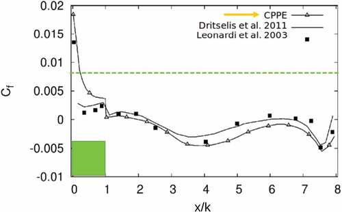
Previously (Leonardi et al., 2003) computed C_f for cases with ribs-like protuberances and reported that normalised perturbations separation of w/k = 7 brought about maximum decrease of the skin friction coefficient, at least in comparison with values of C_f obtained for a plane channel flow with the same bulk velocity. Changes of the skin friction coefficient obtained in our numerical experiments and measured along the separation are presented in Figure 25. The negative values of C_f along the wall in the separation allow to infere the presence of adverse pressure gradients. This particular feature is commonly linked to an augmentation of the form drag, as discussed by (Leonardi et al., 2003).

4.2.2. Mean and fluctuation velocities

In Figure 26 velocity profiles in streamwise direction obtained with our SGS model implementation and the profiles obtained by (Leonardi et al., 2003) and (Dritselis, 2014) are compared. A significant shift of the mean velocity peak value towards the top wall of the channel can be clearly appreciated in Figure 26). This shifting evidences a higher shear stress in the top wall, in comparison with a smooth-wall channel. The later is evidenced when the top wall friction velocity computed for the case with ribs-like protuberances is compared against the smooth-wall channel case: the friction velocities obtained for each case are 0.045 y 0.035, respectively. This is an increase of about 30% on the friction value over the smooth-wall channel case.

The velocity fluctuations obtained for this case are presented in Figure 27. It is remarkably to appreciate how the levels of turbulence are increased as a consequence of the perturbations. Such augmentation occurs for both the near-wall region and the channel centre region in comparison to a smooth-wall channel. In this sense, this kind of perturbations generates a major level of turbulent energy transfer within the flow, despite that wall perturbations were prescribed only at the bottom wall.

Figure 26. Streamwise mean velocity profiles normalised with Uc for the case with ribs-like protuberances. Uc is the velocity in the central line of the channel. Comparison with Dritselis (2014) and (rlandi et al. (2006). CPPE SP: Profile taken over the perturbation. CPPE EP: Profile taken between perturbations

4.2.3. Coherent structures

The behaviour of the coherent structures is generated as a consequence of the turbulent dynamic which govern the flow. Such coherent structures can be used to characterised the influence of the geometric perturbations on the turbulent behaviour of the flow. Therefore, with the aim of identifying this kind of structures, the Q Criterion proposed by Hunt et al. (1988) was used in this paper. The Q Criterion is a mechanism used to identify coherent structures of both vortical and rotational nature. In (Hunt et al., 1988) a vortex is defined as a flow region connected with a positive value of the second invariant of the velocity gradient tensor. Hence, this criterion differentiates the coherent structures formed as a consequence of shear stresses over the flow of those formed as a consequence of proper vortical motions of the flow.

According to the criteria mentioned above, two reference values of Q were selected to visualise the formation of this kind of structures. Therefore, a higher value of Q indicates structures with higher levels of vorticity associated with this type of structures. Contrary, values of Q near to zero indicate structures of vortical nature with a low level of vorticity. For this reason, values of Q = 70 and Q = 5 were selected as representative of high- and low-intensity Q structures.

When Figure 29 is observed, it can be evidenced that this kind of perturbations have an important influence on the formation of coherent structures in comparison to the equivalent smooth channel case (See Figure 28). It can be observed that the ribs-like protuberances generate a region of major level of formations of the coherent structures near the perturbations.

Figure 27. Velocity fluctuations behaviour. Profiles normalised with U_b for the case with ribs-like protuberances. Comparison with Dritselis (2014) and Orlandi et al. (2006). CPPE EP: Profile taken between perturbations

Figure 28. Q-Coherent structures for a smooth-wall channel channel

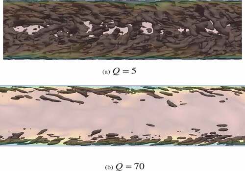
Figure 29. Q-Coherent structures for a channel with ribs-like protuberances

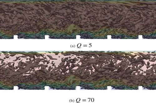
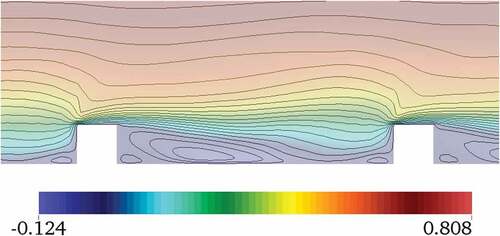
Figure 30. Streamlines for the case with cavity-like perturbations

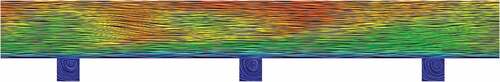
Figure 31. Streamwise mean velocity profile normalised with Uc for the case with cavity-like perturbations. Uc is the velocity in the central line of the channel. Comparison with results obtained with our implementation of the coherent structure SGS model for a plane channel

4.3. Channels with cavity-like wall

4.3.1. Streamlines

In Figure 30 it is observed that there is not any formation of recirculation zones outside the cavities. Nevertheless, inside the cavities, it is clearly observed the well-known lid-driven cavity flow. Such flow presents an oscillatory behaviour, which in consequence generates notable changes in the velocity and pressure fields, as is expressed in (Bouffanais, Deville, Fischer, Leriche, & Weill, 2006; Deshpande & George Milton, 1998, Leriche, 2006; Shankar & Deshpande, 2000).

4.3.2. Velocity profile

Contrary to the observed in the case with ribs-like protuberances, for the case with cavity-like perturbations the shift on the peak value of the velocity profile is not observed. Therefore, in Figure 31 it is remarkable that the maximum velocity value does not show any significant change in comparison to the plane channel case.

4.3.3. Velocity fluctuations

It can be observed in Figure 32, that an attenuation of the velocity fluctuations in the wall-normal and spanwise direction is presented as a consequence of the cavity-like perturbations. In comparison to a plane channel, the reductions of the levels of velocity fluctuations were of 8% y 11,6%, respectively, when such profiles were taken over the perturbations. In contrast, in streamwise direction, it is observed an augmentation on the levels of velocity fluctuations of approximately 17% compared to the plane channel flow. Also is observed that the velocity fluctuations in wall-normal and spanwise direction behave differently when the profiles are taken above and between perturbations.

4.3.4. Coherent structures

For this case, it can be observed in Figure 33 that the cavity-like perturbations generate a decrease in the amount of Q structures formed compared to the plane channel case. This behaviour seems to be related with the behaviour of the velocity fluctuations above mentioned.

5. Conclusions

The present work presents an assessment of the prediction capabilities of two SGS models for Large-Eddy Simulation under OpenFOAM framework. Initially, results for a turbulent flow through smooth-walls channel (or simply smooth-channel) for four different friction Reynolds numbers were compared against LES and DNS data available in the literature. The accuracy of the simulation’s results obtained by an in-house implementation employed showed very good, qualitative and quantitative results when compared to DNS data. This is true for both SGS-models implemented and analysed. The so-called Coherent-Structures model (or simply CS model) was also used to evaluate the turbulent dynamics of flow-through channels with ribs-like protuberances. The results obtained demonstrated that our CS implementation was able to reproduce the main and most important turbulent characteristics of flow featuring regions of high strain-rates and large-scale vortices.

When observing the turbulent flow through the smooth-wall channels, it could be evidenced that in the streamwise direction, the numerical results of velocity fluctuations for both SGS models were consistent. Nevertheless, the Dynamic Smagorinsky (or simply DS) model showed a better performance in the near-wall region, particularly for the lower Reynolds numbers. For higher Reynolds, the differences between the numerical results obtained with both SGS models were insignificant, and both models predicted in a precise manner the profiles of streamwise velocity fluctuations. Regarding velocity fluctuations in wall-normal direction, it was observed that for all the values of Re_τ explored in this work, both models behave similarly. The lowest levels of error were observed for Re_τ = 180. Such behaviour was expected, due to the better grid resolution in this direction.

Assessment of second-order statistics predictions, for both SGS models, showed that both implementations have a high degree of accuracy in the outer region of the boundary layer. Although the viscous dissipation and turbulent production terms obtained for the u^tu^t and u^tv^t components of the Reynolds stress tensor for Re_τ = 180 showed excellent agreement with both experimental and DNS data, the viscous dissipation profiles associated to u^tv^t for flows at Re_τ higher than 180 exhibited a dramatic deviation from experimental data in the sub-viscous layer region. This observation seems to indicate that LES simulations with the DS and CS models need a greater refinement in wall-normal direction than that used in the present work, to accurately predict the behaviour of the smallest scales motions more accurately. As those small-scale motions were not properly captured, it seems obvious to pinpoint this phenomenon as the direct responsible on the reduction of the prediction capabilities of the computational model for the turbulent kinetic energy budget in the aforementioned directions. For low mesh resolution, the viscous dissipation calculation offers low levels of accuracy, particularly, for the cross-component (u^, v^,), where positive values of viscous dissipation could be observed. The later reaffirms the need for high levels of mesh resolution just to obtain acceptable accuracy in the calculation of the viscous dissipation terms. Nevertheless, such a level of refinement is only important in the near-wall region, where the viscous dissipation effects are prominent and relevant.

Figure 32. Velocity fluctuations behaviour. Profiles normalised with U_b for the case with cavity-like perturbations. CPNE EP: Profile taken between perturbations; CPNE SP: Profile taken above perturbations. Comparison with results obtained with our implementation of the coherent structure SGS model for a plane channel

Figure 33. Q Coherent structures for the case with cavity-like perturbations

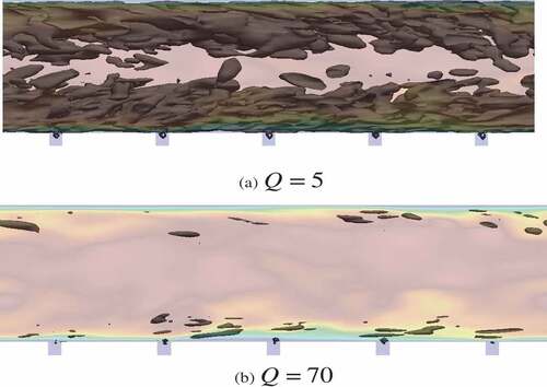
As an alternative and practical application of the implementations explored, a relatively well-known turbulence modulation strategy was studied and analysed. Namely, ribs-like protuberances. In such a case, the influence of these protuberances over the turbulent flow dynamics compared to a smooth-wall or plane channel flow was characterised. It was observed that the ribs-like protuberances generally enhance the turbulent intensity and cavity-like perturbations attenuate the turbulent intensity of the flow. In both cases, the use of coherent structures based on the Q-criterion allowed visualising the effect of the presence of these geometrical features, i.e. ribs-like protuberances and cavity-like perturbations. It is clear then any modulation effect of these features is directly related to the onset and enhancement of regions of high vorticity, and not only due to the generation of regions of high shear stress.

Finally, it is concluded that the implementations of both SGS models under the OpenFOAM framework evaluated in this work had a good performance and excellent prediction capabilities, in general, for the different levels of mesh resolution and Reynolds numbers explored. The later allows to think that these models could be used for practical purposes in different physical an engineering applications. For instance, although an aspect to be carefully considered is the use of a suitable mesh resolution to improve the prediction of viscous dissipation values, both SGS models were able to capture the main turbulent characteristics of the channel flow with a seemingly high level of accuracy.

Acknowledgements

This work was supported by the Universidad Nacional de Colombia under grant [Asistente Docente] and COLCIENCIAS under grant [number 757 Doctorados Nacionales].

We also like to acknowledge Alberto Passalacqua for his invaluable contribution to the implementation of the Dynamic Smagorinsky SGS model over the OpenFOAM Framework.

Data availability

https://drive.google.com/drive/folders/1gezLGzKoOh1JMxsQvAiAxYUSzr5Kdtc2?usp=sharing

Disclosure statement

No potential conflict of interest was reported by the authors.

Additional information

Funding

This work was supported by the COLCIENCIAS [757].

Notes on contributors

Jesus Ramirez-Pastran

The results presented in this paper are part of a project focused on the study of turbulence modulation and the reduction of energy losses due to drag effects, because of the presence of solid particles suspended in turbulent flows in both smooth channels as with geometric disturbances in one of its walls. This project is developed within the GNUM group of the National University of Colombia. The results shown here represent the first step to characterize the effect that solid particles have on the flow turbulent behavior, an aspect that is currently being studied within our research group. The main author of this paper is a mechanical engineer of the Universidad Nacional Experimental del Táchira - Venezuela, with experience in Computational Fluid Dynamics analysis of turbulent flows in engineering applications.

References

- Alletto, M. (2014). Numerical investigation of the influence of particle–particle and particle–wall collisions in turbulent wall–bounded flows at high mass loadings.
- Bardino, J., Ferziger, J. H., & Reynolds, W. C. (1983). Improved turbulence models based on large eddy simulation of homogeneous, incompressible turbulent flows. Technical-Representative.
- Bernardini, M., Pirozzoli, S., & Orlandi, P. (2014). Velocity statistics in turbulent channel flow up to Reτ = 4000. Journal of Fluid Mechanics, 742, 171–39. doi:10.1017/jfm.2013.674
- Bogey, C., & Bailly, C. (2006). Large eddy simulations of round free jets using explicit filtering with/without dynamic Smagorinsky model. International Journal of Heat and Fluid Flow, 27(4), 603–610. doi:10.1016/j.ijheatfluidflow.2006.02.008
- Bose, S. T., Moin, P., & You, D. (2010). Grid-independent large-eddy simulation using explicit filtering. Physics of Fluids, 22(10), 105103. doi:10.1063/1.3485774
- Bouffanais, R., Deville, M. O., Fischer, P. F., Leriche, E., & Weill, D. (2006). Large-eddy simulation of the lid-driven cubic cavity flow by the spectral element method. Journal of Scientific Computing, 27(1), 151–162. doi:10.1007/s10915-005-9039-7
- Chamorro, L. P., Arndt, R. E. A., & Sotiropoulos, F. (2013). Drag reduction of large wind turbine blades through riblets: Evaluation of riblet geometry and application strategies. Renewable Energy, 50, 1095–1105. doi:10.1016/j.renene.2012.09.001
- Choi, K.-S., & Fujisawa, N. (1993). Possibility of drag reduction using d-type roughness. Applied scientific research (pp. 315–324). Springer.
- Churchfield, M. J., Sang, L., & Moriarty, P. J. (2013). Adding complex terrain and stable atmospheric condition capability to the OpenFOAM-based flow solver of the simulator for on/offshore wind farm applications (SOWFA) Tech. rep. National Renewable Energy Lab. (NREL), Golden, CO.
- Clark, R. A., Ferziger, J. H., & Reynolds, W. C. (1979). Evaluation of subgrid-scale models using an accurately simulated turbulent flow. Journal of Fluid Mechanics, 91(01), 1–16. doi:10.1017/S002211207900001X
- Da Silva, C. B., & M´etais, O. (2002). On the influence of coherent structures upon interscale interactions in turbulent plane jets. Journal of Fluid Mechanics, 473, 103–145. doi:10.1017/S0022112002002458
- De Villiers, E. (2006). The potential of large eddy simulation for the modeling of wall bounded flows. In Imperial college of science. London (UK): Technology and Medicine.
- De Villiers, E. (2007). The potential of large eddy simulation for the modelling of wall bounded flows (PhD thesis). University of London.
- Dean, R. B. (1978). Reynolds number dependence of skin friction and other bulk flow variables in two-dimensional rectangular duct flow. Journal of Fluids Engineering, 100(2), 215–223. doi:10.1115/1.3448633
- Del A´lamo, J. C., Jimnez, J., Zandonade, P., & Moser, R. D. (2004). Scaling of the energy spectra of turbulent channels. Journal of Fluid Mechanics, 500, 135–144. doi:10.1017/S002211200300733X
- Deshpande, M. D., & George Milton, S. (1998). Kolmogorov scales in a driven cavity flow. Fluid Dynamics Research, 22(6), 359–381. doi:10.1016/S0169-5983(97)00043-9
- Doolan, C. 2009. “Flow and noise simulation of the NASA tandem cylinder experiment using OpenFOAM”. In: 15th AIAA/CEAS Aeroacoustics Conference (30th AIAA Aeroacoustics Conference) (pp. 3157).
- Dritselis, C. D. (2014). Large eddy simulation of turbulent channel flow with transverse roughness elements on one wall. International Journal of Heat and Fluid Flow, 50, 225–239. doi:10.1016/j.ijheatfluidflow.2014.08.008
- Dritselis, C. D., & Vlachos, N. S. (2011a). Large eddy simulation of gas-particle turbulent channel flow with momentum exchange between the phases. International Journal of Multiphase Flow, 37(7), 706–721. doi:10.1016/j.ijmultiphaseflow.2011.01.012
- Dritselis, C. D., & Vlachos, N. S. (2011b). Numerical investigation of momentum exchange between particles and coherent structures in low Re turbulent channel flow. Physics of Fluids, 23(2), 025103. doi:10.1063/1.3553292
- Dubois, T., & Bouchon, F. (1998). Subgrid-scale models based on incremental unknowns for large eddy simulation. Center for Turbulence Research Annual Research Briefs, 221–236.
- El-Samni, O. A., Chun, H. H., & Yoon, H. S. (2007). Drag reduction of turbulent flow over thin rectangular riblets. International Journal of Engineering Science, 45(2–8), 436–454. doi:10.1016/j.ijengsci.2007.03.002
- Flores, F., Garreaud, R., & Mun˜oz, R. C. (2014). OpenFOAM applied to the CFD simulation of turbulent buoyant atmospheric flows and pollutant dispersion inside large open pit mines under intense insolation. Computers & Fluids, 90, 72–87. doi:10.1016/j.compfluid.2013.11.012
- Fran, C. K., & Bogey, C. (2015). Large-eddy simulation of turbulent channel flow using relaxation filtering: Resolution requirement and Reynolds number effects. Computers & Fluids, 116, 17–28. doi:10.1016/j.compfluid.2015.03.026
- Garc´ıa-Mayoral, R., & Jim´enez, J. (2011). Drag reduction by riblets. Philosophical Transactions of the Royal Society of London A: Mathematical, Physical and Engineering Sciences, 369(1940), 1412–1427. doi:10.1098/rsta.2010.0359
- Germano, M., Piomelli, U., Moin, P., & Cabot, W. H. (1991). A dynamic subgrid-scale eddy viscosity model. Physics of Fluids A: Fluid Dynamics, 3(7), 1760–1765. doi:10.1063/1.857955
- Girimaji, S., & Abdol-Hamid, K. 2005. Partially-averaged Navier Stokes model for turbulence: Implementation and validation. In: 43rd AIAA Aerospace Sciences Meeting and Exhibit (pp. 502).
- Gloerfelt, X., & Berland, J. (2013). Turbulent boundary-layer noise: Direct radiation at mach number 0.5. Journal of Fluid Mechanics, 723, 318–351. doi:10.1017/jfm.2013.134
- Higuera, P., Lara, J. L., & Losada, I. J. (2014). Three-dimensional interaction of waves and porous coastal structures using OpenFOAM R. Part I: Formulation and validation. Coastal Engineering, 83, 243–258.
- Hoyas, S., & Jim´enez, J. (2006). Scaling of the velocity fluctuations in turbulent channels up to Re τ = 2003. Physics of Fluids, 18(1), 011702. doi:10.1063/1.2162185
- Hunt, J. C. R., Wray, A. A., & Moin, P. (1988). Eddies, streams, and conver- gence zones in turbulent flows.
- Inagaki, M., Kondoh, T., & Nagano, Y. (2005). A mixed-time-scale SGS model with fixed model-parameters for practical LES. Journal of Fluids Engineering, 127(1), 1–13. doi:10.1115/1.1852479
- Islam Mallik, M. S., Uddin, M. A., & Meah, M. A. (2014). Large eddy simulation of turbulent channel flow at Reτ = 590. IOSR–Journal of Math- Ematics, 10(6), 41–50. doi:10.9790/5728
- Jacobsen, N. G., Fuhrman, D. R., & Fredsøe, J. (2012). A wave generation toolbox for the open-source CFD library: OpenFoam. International Journal for Numerical Methods in Fluids, 70(9), 1073–1088. doi:10.1016/j.coastaleng.2013.08.010
- Jiménez, J., Wray, A. A., Saffman, P. G., & Rogallo, R. S. (1993). The structure of intense vorticity in isotropic turbulence. Journal of Fluid Mechanics, 255, 65–90. doi:10.1017/S0022112093002393
- John, V. (2012). Large eddy simulation of turbulent incompressible flows: Analytical and numerical results for a class of LES models (Vol. 34). Springer Science & Business Media.
- Kajishima, T., & Nomachi, T. (2006). One-equation subgrid scale model using dynamic procedure for the energy production. Journal of Applied Mechanics, 73(3), 368–373. doi:10.1115/1.2164509
- Kim, J., Moin, P., & Moser, R. (1987). Turbulence statistics in fully de- veloped channel flow at low Reynolds number. Journal of Fluid Mechanics, 177, 133–166. doi:10.1017/S0022112087000892
- Kleissl, J., Kumar, V., Meneveau, C., & Parlange, M. B. (2006). Numerical study of dynamic Smagorinsky models in large- eddy simulation of the atmospheric boundary layer: Validation in stable and unstable conditions. Water Resources Research, 42(6). doi:10.1029/2005WR004685
- Kobayashi, H. (2005). The subgrid-scale models based on coherent structures for rotating homogeneous turbulence and turbulent channel flow. Physics of Fluids, 17(4), 045104. doi:10.1063/1.1874212
- Kobayashi, H. (2006). Large eddy simulation of magnetohydrodynamic turbu- lent channel flows with local subgrid-scale model based on coherent structures. Physics of Fluids, 18(4), 045107. doi:10.1063/1.2194967
- Kobayashi, H., Ham, F., & Wu, X. (2008). Application of a local SGS model based on coherent structures to complex geometries. International Journal of Heat and Fluid Flow, 29(3), 640–653. doi:10.1016/j.ijheatfluidflow.2008.02.008
- Kravchenko, A. G., & Moin, P. (2000). Numerical studies of flow over a circular cylinder at Re D= 3900. Physics of Fluids, 12(2), 403–417. doi:10.1063/1.870318
- Lee, M., & Moser, R. D. (2014). Direct numerical simulation of turbulent channel flow up to Reτ approx 5200. Journal of Fluid Mechanics, 774, 395–415
- Lee, M., & Moser, R. D. (2015). Direct numerical simulation of turbulent channel flow up to Reτ approx 5200. Journal of Fluid Mechanics, 774, 395–415. doi:10.1017/jfm.2015.268
- Leonardi, S., Orlandi, P., & Antonia, R. A. (2005). A method for determining the frictional velocity in a turbulent channel flow with roughness on the bottom wall. Experiments in Fluids, 38(6), 796–800. doi:10.1007/s00348-005-0975-7
- Leonardi, S., Orlandi, P., Djenidi, L., & Antonia, R. A. (2004). Structure of turbulent channel flow with square bars on one wall. International Journal of Heat and Fluid Flow, 25(3), 384–392. doi:10.1016/j.ijheatfluidflow.2004.02.022
- Leonardi, S., Orlandi, P., Smalley, R. J., Djenidi, L., & Antonia, R. A. (2003). Direct numerical simulations of turbulent channel flow with transverse square bars on one wall. Journal of Fluid Mechanics, 491, 229–238. doi:10.1017/S0022112003005500
- Leonardi, S., Orlandi, P., & Antonia, R. A. (2007). Properties of d-and k-type roughness in a turbulent channel flow. Physics of Fluids, 19(12), 125101. doi:10.1063/1.2821908
- Leriche, E. (2006). Direct numerical simulation in a lid-driven cubical cavity at high Reynolds number by a Chebyshev spectral method. Journal of Scientific Computing, 27(1), 335–345. doi:10.1007/s10915-005-9032-1
- Lesieur, M., & Metais, O. (1996). New trends in large-eddy simulations of turbulence. Annual Review of Fluid Mechanics, 28(1), 45–82. doi:10.1146/annurev.fl.28.010196.000401
- Lilly, D. K. (1992). A proposed modification of the Germano subgrid-scale closure method. Physics of Fluids A: Fluid Dynamics, 4(3), 633–635. doi:10.1063/1.858280
- Luo, D. D., Leung, C. W., Chan, T. L., & Wong, W. O. (2005). Flow and forced-convection characteristics of turbulent flow through parallel plates with periodic transverse ribs. Numerical Heat Transfer, Part A: Applications, 48(1), 43–58. doi:10.1080/10407780590929829
- Lysenko, D. A., Ertesv°ag, I. S., & Rian, K. E. (2013). Modeling of turbulent separated flows using OpenFOAM. Computers & Fluids, 80, 408–422. doi:10.1016/j.compfluid.2012.01.015
- Lysenko, D. A., Ertesv°ag, I. S., & Rian, K. E. (2012). Large-eddy simulation of the flow over a circular cylinder at Reynolds number 3900 using the Open- FOAM toolbox. Flow, Turbulence and Combustion, 89(4), 491–518. doi:10.1007/s10494-012-9405-0
- Mallouppas, G., & van Wachem, B. (2013). Large eddy simulations of turbulent particle-laden channel flow. International Journal of Multiphase Flow, 54, 65–75. doi:10.1016/j.ijmultiphaseflow.2013.02.007
- Marchioli, C. (2017). Large-eddy simulation of turbulent dispersed flows: A review of modelling approaches. Acta Mechanica, 228(3), 741–771. doi:10.1007/s00707-017-1803-x
- Meyers, J., & Sagaut, P. (2007). Is plane-channel flow a friendly case for the testing of large-eddy simulation subgrid-scale models? Physics of Fluids, 19(4), 048105. doi:10.1063/1.2722422
- Moeng, C. H., & Sullivan, P. P. (2015). Large-eddy simulation. Encyclopedia of Atmospheric Sciences, 2, 232–240.
- Moin, P., & Kim, J. (1982). Numerical investigation of turbulent channel flow. Journal of Fluid Mechanics, 118, 341–377. doi:10.1017/S0022112082001116
- Moser, R. D., Kim, J., & Mansour, N. N. (1999). Direct numerical simulation of turbulent channel flow up to Re τ = 590. Physics of Fluids, 11(4), 943–945. doi:10.1063/1.869966
- Muntean, S., Nilsson, H., & Susan-Resiga, R. F. (2009 October). “3D numerical analysis of the unsteady turbulent swirling flow in a conical diffuser using fluent and OpenFOAM”. In: Proceedings of the 3rd IAHR International Meeting of the Workgroup on Cavitation and Dynamic Problems in Hydraulic Machinery and Systems (pp. 14–16), Brno, Czech Republic.
- Nadeem, M., Lee, J. H., Lee, J., & Sung, H. J. (2015). Turbulent boundary layers over sparsely-spaced rod- roughened walls. International Journal of Heat and Fluid Flow, 56, 16–27. doi:10.1016/j.ijheatfluidflow.2015.06.006
- Nagano, Y., Hattori, H., & Houra, T. (2004). DNS of velocity and thermal fields in turbulent channel flow with transverse-rib roughness. International Journal of Heat and Fluid Flow, 25(3), 393–403. doi:10.1016/j.ijheatfluidflow.2004.02.011
- Nilsson, H. (2007, November 26–27). “Experiences with OpenFOAM for water turbine applications”. In: Proceedings of the 1st OpenFOAM International Conference, Beaumont House, Old Windsor, United Kingdom.
- Orlandi, P., Leonardi, S., & Antonia, R. A. (2006). Turbulent channel flow with either transverse or longitudinal roughness elements on one wall. Journal of Fluid Mechanics, 561, 279–305. doi:10.1017/S0022112006000723
- Panjwani, B., Popescu, M., Samseth, J., Meese, E., & Mahmoudi, J. (2014). OffWindSolver: Wind farm design tool based on actuator line/actuator disk concept in OpenFoam architecture. In ITM Web of Conferences (Vol. 2, p. 04001). EDP Sciences.
- Pantano, C., Pullin, D. I., Dimotakis, P. E., & Matheou, G. (2008). LES approach for high Reynolds number wall-bounded flows with application to turbulent channel flow. Journal of Computational Physics, 227(21), 9271–9291. doi:10.1016/j.jcp.2008.04.015
- Peltola, J., Pättikangas, T., Brockmann, T., Siikonen, T., Toppila, T., & Brandt, T. (2011, May). Adaptation and validation of OpenFOAM® CFD-solvers for nuclear safety related flow simulations. In SAFIR2010 Seminar (Vol. 17, No. 2011, pp. 1-20).
- Piomelli, U. (2014). Large eddy simulations in 2030 and beyond. Philosophical Transactions of the Royal Society A, 372(2022), 20130320. doi:10.1098/rsta.2013.0320
- Robertson, E., Choudhury, V., Bhushan, S., & Walters, D. K. (2015). Validation of OpenFOAM numerical methods and turbulence models for incompressible bluff body flows. Computers & Fluids, 123, 122–145. doi:10.1016/j.compfluid.2015.09.010
- Sagaut, P. (2006). Large eddy simulation for incompressible flows: An introduction. Springer Science & Business Media.
- Saha, A. K., & Acharya, S. (2004). Unsteady simulation of turbulent flow and heat transfer in a channel with periodic array of cubic pin-fins. Numerical Heat Transfer, Part A: Applications, 46(8), 731–763. doi:10.1080/104077890504465
- Saidi, B. S. A. (2000). Numerical simulation of turbulent convective heat transfer in square ribbed ducts. Numerical Heat Transfer: Part A: Applications, 38(1), 67–88. doi:10.1080/10407780050134974
- Schiavo, L. A. C. A., Wolf, W. R., & Azevedo, J. L. F. (2017). Turbulent kinetic energy budgets in wall bounded flows with pressure gradients and separation. Physics of Fluids, 29(11), 115108. doi:10.1063/1.4992793
- Schlatter, P., Li, Q., Brethouwer, G., Johansson, A. V., & Henningson, D. S. (2010). Simulations of spatially evolving turbulent boundary layers up to Reθ = 4300. International Journal of Heat and Fluid Flow, 31(3), 251–261. doi:10.1016/j.ijheatfluidflow.2009.12.011
- Shankar, P. N., & Deshpande, M. D. (2000). Fluid mechanics in the driven cavity. Annual Review of Fluid Mechanics, 32(1), 93–136. doi:10.1146/annurev.fluid.32.1.93
- Smagorinsky, J. (1963). General circulation experiments with the primitive equations: I. The basic experiment. Monthly Weather Review, 91(3), 99–164. doi:10.1175/1520-0493(1963)091<0099:GCEWTP>2.3.CO;2
- Taylor, G. I., Maccoll, J. W., & Durand, W. F. (1935). Aerodynamic Theory. Julius Springer, Berlin, 3, 209.
- Veloudis, I., Yang, Z., & McGuirk, J. J. (2008). LES of wall-bounded flows using a new subgrid scale model based on energy spectrum dissipation. Journal of Applied Mechanics, 75(2), 021005. doi:10.1115/1.2775499
- Viazzo, S., Dejoan, A., & Schiestel, R. (2001). Spectral features of the wall-pressure fluctuations in turbulent wall flows with and without perturba- tions using LES. International Journal of Heat and Fluid Flow, 22(1), 39–52. doi:10.1016/S0142-727X(00)00074-6
- Vincent, A., & Meneguzzi, M. (1991). The spatial structure and statistical properties of homogeneous turbulence. Journal of Fluid Mechanics, 225, 1–20. doi:10.1017/S0022112091001957
- Vreman, A. W. (2004). An eddy-viscosity subgrid-scale model for turbulent shear flow: Algebraic theory and applications. Physics of Fluids, 16(10), 3670–3681. doi:10.1063/1.1785131
- Yoshizawa, A., Kobayashi, K., Kobayashi, T., & Taniguchi, N. (2000). A nonequilibrium fixed-parameter subgrid-scale model obeying the near-wall asymptotic constraint. Physics of Fluids, 12(9), 2338–2344. doi:10.1063/1.1287518
- Zhiwei, H., Morfey, C. L., & Sandham, N. D. (2006). Wall pressure and shear stress spectra from direct simulations of channel flow. AIAA Journal, 44(7), 1541–1549. doi:10.2514/1.17638
- Zhiyin, Y. (2015). Large-eddy simulation: Past, present and the future. Chinese Journal of Aeronautics, 28(1), 11–24. doi:10.1016/j.cja.2014.12.007