Uncertainty quantification of model predictive control for nonlinear systems with parametric uncertainty using hybrid pseudo-spectral method

Abstract

In this paper, a hybrid pseudo-spectral (hPS) method is utilized to analyze the uncertainty of the model predictive control (MPC) for nonlinear systems with stochastic parameter uncertainty. The hPS method incorporates Generalized polynomial expansion (gPC) and pseudo-spectral (PS) optimal control in a hybrid format. To quantify the effect of uncertainty on the MPC states and control inputs, we use the gPC method, and for time discretization of the MPC problem, the pseudo-spectral method is employed. The proposed method will be compared with the well-known Monte Carlo (MC) simulation method in terms of computational speed. Two dynamical systems are tested. First, an industrial process, continuous stirred reactor tank, which is a highly nonlinear system, with Gaussian distributed parameter uncertainty and second, a typical second-order dynamical system with uniform and Weibull distributed parameter uncertainty. Simulation results demonstrate that the proposed method can approximate the two first moments of the states and control inputs under MPC much faster and computationally more efficient than MC simulations.

Keywords:

• model predictive control
• uncertainty analysis
• Generalized Polynomial Chaos
• pseudo-spectral optimal control

PUBLIC INTEREST STATEMENT

Uncertainty quantification is the science of quantitative characterization of uncertainties in real-world applications. It tries to determine how likely certain outcomes are if some aspects of the system are not exactly known. Most practical systems are exposed to uncertainty and engineers need to know how the uncertainty will affect the system. In this paper, we proposed a hybrid pseudo-spectral algorithm to quantify the effect of uncertainty on nonlinear systems under a model predictive control strategy.

1. Introduction

MPC is one of the most practical methods of advanced process control in the industry. It is an optimal control strategy that is implemented in a receding horizon manner. By implementing the MPC strategy, certain constraints can be imposed on outputs, inputs, and states of the system. Furthermore, it can be implemented on both linear and nonlinear dynamical systems. Many applications of linear MPC have been reported in the literature (Garcia, Prett, & Morari, 1989; Muske & Rawlings, 1993; Schwickart, Voos, Hadji‐Minaglou, & Darouach, 2016; Widd, Liao, Gerdes, Tunestål, & Johansson, 2014). For some highly nonlinear systems, the approximated linear model is not sufficient. Therefore, the MPC should be designed directly based on the nonlinear model (Grüne & Pannek, 2011; Mayne, Rawlings, Rao, & Scokaert, 2000). Several theories have been proposed regarding the stability and feasibility of the MPC, both in linear and nonlinear context. In nonlinear MPC (NMPC), the system or constraints are nonlinear. The efforts to prove the stability of NMPC have led to the well-known four axioms of stability (Mayne et al., 2000). Such as nonlinearity, which is the inherent characteristic of real-world systems, parameter uncertainties occur in many practical systems. Uncertainties in the parameters of a system could either be bounded or have a stochastic nature.

When the uncertainty is bounded, the well-known robust MPC strategies are applied. Tube-based MPC is a dominant approach in this field (Mayne, Kerrigan, Van Wyk, & Falugi, 2011). For systems with stochastic parameter uncertainty, where the probability distribution of uncertainty is known, the stochastic MPC strategies are employed. In Visintini, Glover, Lygeros, and Maciejowski (2006), the Markov-chain Monte Carlo technique was proposed for solving constrained nonlinear stochastic optimization problems. In Bavdekar and Mesbah (2016), at each sampling time of the MPC, the gPC coefficients were calculated and then the MPC was performed on the gPC coefficients. The Fokker–Planck equation, which described the probability density of the states of the system, was utilized in Annunziato and Borzì (2013) to solve the MPC for the stochastic differential equation. In Annunziato and Borzì (2013), the MPC for the system of stochastic differential equations was transformed into a deterministic MPC with PDE constraint. The stochastic Lyapunov function was considered as an auxiliary constraint in the stochastic MPC framework in Mahmood and Mhaskar (2012) to guarantee the stochastic stability of the SDE under MPC strategy.

Control engineers should always have a general sight of the effects of uncertainty on the system under the MPC strategy. By analyzing the uncertainty effects on the system, one can choose the system hardware and software accordingly. For instance, the effect of the uncertainty on the control actuation can be evaluated and the size of the actuator can be determined. Uncertainty quantification is the science of quantitative characterization of uncertainties in real-world applications. It tries to determine how likely certain outcomes are if some aspects of the system are not exactly known. This paper is the continuation of our previous work (Namadchian & Ramezani, 2017) in which we used the pseudo-spectral method for time discretization of the MPC for a CSTR and showed the computational efficiency of the proposed method compared with RK4 time discretization method. In this paper, we have not only used the PS method for time discretization but also applied gPC, for uncertainty quantification and propose a hybrid pseudo-spectral method for uncertainty quantification of nonlinear MPC.

Pseudo-spectral methods referred to a class of spectral techniques which are solved by collocation points (Fornberg, 1998). In this paper, for uncertainty propagation in nonlinear MPC, the Generalized Polynomial Chaos (Xiu & Karniadakis, 2002) has been utilized. GPC is a very efficient spectral method for uncertainty evaluation. In the sample-based version of the gPC or collocation-based gPC, the uncertainty can be analyzed with much fewer samples than Monte Carlo (MC) simulations.

The proposed hybrid algorithm selects samples from the random space using collocation nodes, after that, inserts those sample values into the differential equations of the system, and then uses a pseudo-spectral based deterministic solver to generate solutions for each of the resulting deterministic problems.

The set of deterministic solutions is then used to construct a polynomial representation of the solution of the stochastic optimal control problem using the gPC method. Since both gPC and PS optimal control can be categorized as PS methods and are incorporated in a hybrid format, we call this approach, the hybrid pseudo-spectral or the hPS method.

PS optimal control is an efficient computational method for solving optimal control problems. The most advanced optimal control softwares such as GPOPS, PSOPT, and RPROPT use PS optimal control to discretize the nonlinear optimal control problem and transform it into a nonlinear programming problem (Becerra, 2010; Patterson & Rao, 2014.

The hybrid method, involving a combination of the PS optimal control and gPC, has been appeared in few publications. Harmon (2017) utilized the PS optimal control with gPC to quantify the effect of uncertainty on the optimal states of the system. Matsuno, Tsuchiya, Wei, Hwang, and Matayoshi (2015) solved the aircraft conflict resolution by the hPS. The system was a 3D aircraft dynamic under wind uncertainty. The main goal of the optimal control problem was to determine the optimal trajectories in a way that the confliction of the aircraft is avoided. The conflict was modeled as the distance between two aircraft and as a constraint in the optimal control problem, the distance must not exceed a predefined threshold value. Motivated by his previous work, Matsuno developed his approach for aircraft conflict resolution for online applications (Matsuno, Tsuchiya, & Matayoshi, 2015). By Polynomial Chaos Kriging method, he constructed a surrogate model for the solution of stochastic optimal control method based on the hPS. Then, the surrogate model was used to circumvent the need for solving a stochastic optimal control problem on-line. Although the mentioned papers utilized both PS optimal control and gPC in a hybrid manner, they did not address the optimal control problem in a receding horizon approach, i.e. MPC framework. What distinguishes our work from these papers is considering the uncertainty quantification of optimal control in a receding horizon manner. The main contribution of our work is to quantify the effect of parameter uncertainty on the states and controls of the nonlinear system under MPC strategy with less computational effort than MC simulations.

The paper is structured as follows: Section 2 gives details on the problem formulation and notations. The PS fundamentals are described in Section 3. The polynomial chaos theory is introduced in Section 4. The hybrid PS-MPC uncertainty propagation algorithm is presented in Section 5. In Section 6, uncertainty evaluation is performed on two examples under MPC strategy and compared with MC simulations.

2. Problem formulation

Consider the following continuous-time system in the state space form:

(1) $\dot{x}(t)=F(x(t),u(t),\theta )$(1)

Since in MPC literature, the control is normally piecewise constant, without loss of generality, we can always express the system (1) with a difference equation by an appropriate sampling time $\mathrm{\Delta }t$ could be expressed as follows:

(2) $x(k+1)=f(x(k),u(k),\theta )$(2)

where $x(k)\in {\mathbb{R}}^{n_x}$ is the state of the system at time index $k$, $u(k)\in {\mathbb{R}}^{n_u}$ is the manipulated input, $\theta \in {\mathbb{R}}^{n_{\theta }}$ is the vector of unknown parameters. $\theta$ is stochastic uncertainty. ${\theta }_i$, the component of $\theta$ are assumed to be independent and identically distributed random variables with pdf $f_{{\theta }_i}$ such that ${\theta }_i\in K\subset L^2(\mathrm{\Omega },F,P)$, $(\mathrm{\Omega },F,P)$ is the probability space, $\mathrm{\Omega }$ is the sample space, $F$ is the $\sigma -algebra$ of the events, and $P$ is the probability measure of events. The first moment or expectation of a random variable $\theta$ is defined as $E(\theta )={\int }_{\mathrm{\Omega }}\theta (w)dP(w)$. $L^2(\mathrm{\Omega },F,P)$ is the Hilbert space of all random variables $\theta$ whose $L_2-norm$ is finite, i.e. $||\theta |{|}_2=E[|\theta {|}^2{]}^{1/2}<\mathrm{\infty }$. Also, the second moment of $\theta$, called variance, is defined as $Var(\theta )=E[(\theta -E[\theta ]{)}^2]={\sigma }_{\theta }^2$, where ${\sigma }_{\theta }$ is the standard deviation. We assume that $f$ is continuously differentiable with respect to its arguments and the solution of (2) exists uniquely and almost surely.

The MPC formulation for Equation (2)(2) $x(k+1)=f(x(k),u(k),\theta )$(2) is as follows:

(3) ${\min }_{U(t)}{V}_N(x,u,\theta )=V_f(x(N|t))+{\displaystyle \sum _{k=0}^{N_p-1}l}(x(k|t),u(k|t))$(3)

$subjectto:$

(4) $x(k+1|t)=f(x(k|t),u(k|t),\theta )$(4)

(5) $x(k|t)\in \mathbb{X}k=1,...,N_p$(5)

(6) $u(k|t)\in \mathbb{U}k=0,...,N_c$(6)

(7) $x(N|t)\in {\mathbb{X}}_f$(7)

(8) $x(0|t)=x(t)$(8)

where $x(k|t)$ is the predicted value of $x$, $k$ step ahead of $t$, based on the information available at time $t$. $N_p$ and $N_c$ are prediction and control horizons, respectively. $\mathbb{X}$ and $\mathbb{U}$ are state and control constraints, respectively, and ${\mathbb{X}}_f$ is the terminal constraint. $V_N(x,u)$, the cost function, consists of the stage cost $l(x,u)$ and the terminal cost $V_f(x)$.

It is assumed that at each step, the states of the system $x(k)$ are measurable. Due to the randomness of $\theta$, $x(k)$ and $u(k)$ are stochastic processes. Our goal is to find the mean and variance of the states and control inputs at each time index $k$ to find how the randomness of $\theta$ will affect the distribution of control inputs and the states of the uncertain system under the MPC strategy.

The terminal constraint (7) imposes an implicit constraint on the control sequence of the form:

$u\in {\mathcal{U}}_N(x,\theta )$

where the control constraint set ${\mathcal{U}}_N(x,\theta )$ is the set of control sequence $u:=\{u(0),u(1),...,u(N-1)\}$ satisfying the state and control constraints:

${\mathcal{U}}_N(x,\theta ):=\{u|(x,u)\in {\mathcal{Z}}_N(\theta )\}$

where ${\mathcal{Z}}_N(\theta )\subset {\mathbb{R}}^n\times {\mathbb{R}}^{Nm}$ is defined by

${\mathcal{Z}}_N(\theta )=\{(x,u)|u(k)\in \mathbb{U},x(k)\in \mathbb{X},\mathrm{\forall }k\in \left\{0,1,\dots ,N-1\right\}andx(N)\in {\mathbb{X}}_f(\theta )\}$

Therefore, the optimal control problem ${\mathcal{P}}_N(x,\theta )$ is defined as:

${\mathcal{P}}_N(x,\theta ):V_N^0(x,\theta )=\underset{u}{min}\{V_N(x,u,\theta )|u\in {\mathcal{U}}_N(x,\theta )\}$

The following assumptions are considered for the MPC controller:

Assumption 1.

1. Continuity of the system: for each ${\theta }_i\in K\subset L^2(\mathrm{\Omega },F,P)$, the function $f:\mathbb{X}\times \mathbb{U}\to {\mathbb{R}}^{n_x}$, $l:\mathbb{X}\times \mathbb{U}\to {\mathbb{R}}_{\ge 0}$, and $V_f:\mathbb{X}\to {\mathbb{R}}_{\ge 0}$ are continuous and $f(0,0,{\theta }_i)=0$, $V_f(0,{\theta }_i)=0$, $l(0,0)=0$ and $l(.,.)$ is strictly positive function.

2. Properties of the constraint set: for each ${\theta }_i\in K\subset L^2(\mathrm{\Omega },F,P)$, the set $\mathbb{X}$ and ${\mathbb{X}}_f({\theta }_i)$ are closed, ${\mathbb{X}}_f({\theta }_i)\in \mathbb{X}$ and $\mathbb{U}$ are compact, each set contains the origin.

Theorem.1 (axioms of stability for MPC) (Mayne et al., 2000):

If for any ${\theta }_i\in K\subset L^2(\mathrm{\Omega },F,P)$, the following assumptions are satisfied, then the states of the system $f(x,u,{\theta }_i)$ converge asymptotically to the origin under MPC formulation ${\mathcal{P}}_N(x,{\theta }_i)$:

A1: State constraint satisfied in ${\mathbb{X}}_f({\theta }_i)$:

${\mathbb{X}}_f({\theta }_i)\subset \mathbb{X}$, ${\mathbb{X}}_f({\theta }_i)$ closed. $0\in {\mathbb{X}}_f({\theta }_i)$

A2: Control constraint satisfied in ${\mathbb{X}}_f({\theta }_i)$ .

There exists a local controller ${\kappa }_f(x,{\theta }_i)$, such that ${\kappa }_f(x,{\theta }_i)\in \mathbb{U}$. $\mathrm{\forall }x\in {\mathbb{X}}_f$ (${\kappa }_f(x,{\theta }_i)$ is a local feedback controller on ${\mathbb{X}}_f({\theta }_i)$)

A3: ${\mathbb{X}}_f({\theta }_i)$ is positively invariant under ${\kappa }_f(x,{\theta }_i)$

$f(x,{\kappa }_f(x,{\theta }_i))\in {\mathbb{X}}_f({\theta }_i),\mathrm{\forall }x\in {\mathbb{X}}_f({\theta }_i)$

A4: $V_f(x,{\theta }_i)$ is a local Lyapunov function:

$[V_f(f(x,{\kappa }_f(x,{\theta }_i)))-V_f(x,{\theta }_i)+l(x,{\kappa }_f(x,{\theta }_i))]\le 0$

Proof:

In the axioms of stability for the MPC, we consider ${\mathbb{X}}_f({\theta }_i)$, $V_f(x,{\theta }_i)$, ${\kappa }_f(x,{\theta }_i)$ such that the axioms are satisfied for each ${\theta }_i$, so without loss of generality, to prove the theorem, we consider ${\theta }_i$ as a constant and omit it from the equations.

The stability of the MPC will be proved based on using the value function as a decreasing Lyapunov like function. In the first part, we prove that initial feasibility implies recursive feasibility and in the second part, the convergence of the system to the origin will be guaranteed under MPC strategy.

Part 1- recursive feasibility

Suppose ${\mathcal{P}}_N(x)$ has a feasible solution at time $k$, i.e. $u=\{u^{\ast }(0),u^{\ast }(1),...,u^{\ast }(N-1)\}$ is the optimal control solution that satisfies the control, state, and the terminal constraint. Let $x=\{x^{\ast }(0),x^{\ast }(1),...,x^{\ast }(N)\}$ denotes the optimal control trajectories. Implementing $u^{\ast }\{0\}$ as a feasible control to the system, steers the initial state to the successor state $x^{+}=x(k+1)=f(x(k),u\{0\})$. For ${\mathcal{P}}_N(x^{+})$, we want to find the feasible control sequence. Since $\tilde{u}=\{u^{\ast }(1),...,u^{\ast }(N-1)\}$ steers $x^{+}$ to $x(N)\in {\mathbb{X}}_f$, to obtain the feasible control sequence for ${\mathcal{P}}_N(x^{+})$, one further element to $\tilde{u}$ need to be added. If we add $u\{N\}={\kappa }_f(x^{\ast }(N))$ to $\tilde{u}$, since ${\mathbb{X}}_f\subset \mathbb{X}$, ${\kappa }_f(x)\subset \mathbb{U}$ and $f(x,{\kappa }_f(x))\in {\mathbb{X}}_f\mathrm{\forall }x\in {\mathbb{X}}_f$ the control sequence $\tilde{u}=\{u^{\ast }(1),...,u^{\ast }(N-1),{\kappa }_f(x^{\ast }(N))\}$ is feasible for ${\mathcal{P}}_N(x^{+})$, so the initial feasibility gives recursive feasibility.

Part2- Asymptotic stability

The most popular idea in the proof of the stability of the MPC is to show that optimal objective function $V_N^0(x)$ is a Lyapunov function satisfying $V_N^{\ast }(x(t+1))-V_N^{\ast }(x(t))<0,\mathrm{\forall }x\ne 0$

For the optimal control sequence $u=\{u^{\ast }(0),u^{\ast }(1),...,u^{\ast }(N-1)\}$ calculated at $x(t)$, the optimal objective function is:

$V_N^0(x(t))=V_f(x^{\ast }(N))+\sum _{k=0}^{N_p-1}l(x^{\ast }(k),u^{\ast }(k))$

Also, for sub-optimal control sequence $\tilde{u}=\{u^{\ast }(1),...,u^{\ast }(N-1),{\kappa }_f(x^{\ast }(N))\}$ the suboptimal objective function is as follows:

$V_N^{\mathrm{\prime }}(x(t+1))=V_f(f(x^{\ast }(N),{\kappa }_f(x^{\ast }(N))))+\sum _{k=0}^{N_p}l(x^{\ast }(k),u^{\ast }(k))$

Since $V_N^{\mathrm{\prime }}(x)$ is a sub-optimal solution, we have:

$V_N^{\ast }(x)\le V_N^{\mathrm{\prime }}(x)$ and $V_N^{\mathrm{\prime }}(x)$ can be rewritten as follows:

$V_f(f(x^{\ast }(N),{\kappa }_f(x^{\ast }(N))))+\sum _{k=0}^{N_p-1}l(x^{\ast }(k),u^{\ast }(k))-l(x^{\ast }(0),u^{\ast }(0))+l(x^{\ast }(N),{\kappa }_f(x^{\ast }(N)))$

By adding and subtracting $V_f(x^{\ast }(N))$ to the above expression, we obtain:

$\sum _{k=0}^{N_p-1}l(x^{\ast }(k),u^{\ast }(k))+V_f(x^{\ast }(N))-V_f(x^{\ast }(N))-l(x^{\ast }(0),u^{\ast }(0))+V_f(f(x^{\ast }(N),{\kappa }_f(x^{\ast }(N))))+l(x^{\ast }(N),{\kappa }_f(x^{\ast }(N)))$

It can be seen that the first two terms in the above equation is equal to $V_N^{\ast }(x)$, thus we can rewrite it as:

$V_N^{\ast }(x)-l(x^{\ast }(0),u^{\ast }(0))-V_f(x^{\ast }(N))+V_f(f(x^{\ast }(N),{\kappa }_f(x^{\ast }(N))))+l(x^{\ast }(N),{\kappa }_f(x^{\ast }(N)))$

From A4 (MPC axioms of stability), for the last tree term in the above expression we have:

$V_f(f(x^{\ast }(N),{\kappa }_f(x^{\ast }(N))))-V_f(x^{\ast }(N))+l(x^{\ast }(N),{\kappa }_f(x^{\ast }(N)))\le 0$

Leaving us with the expression:

$V_N^{\ast }(x(t+1))-V_N^{\ast }(x(t))\le -l(x^{\ast }(0),u^{\ast }(0)),\mathrm{\forall }x\ne 0$

Since it is assumed that $l(0,0)=0$ and $l(.)$ is a strictly positive function, we have:

$V_N^{\ast }(x(t+1))-V_N^{\ast }(x(t))<0,\mathrm{\forall }x\ne 0$

Indicating that the objective function $V_N^{\ast }(x(t)$ is strictly decreasing along closed-loop trajectories under MPC control, thus the trajectories converge to the origin. ∎

2.1. Design of stable MPC for nonlinear systems

The proper choices of ${\mathbb{X}}_f({\theta }_i)$, $V_f(x,{\theta }_i)$, and ${\kappa }_f(x,{\theta }_i)$ guarantee the asymptotic stability of the MPC.

To design an MPC for the nonlinear system (2), we choose $l(x,u)=(1/2)(|x{|}_Q^2+|u{|}_R^2)$, in which $Q$ and $R$ are positive definite. In order to select a proper $V_f(x,{\theta }_i)$ and ${\mathbb{X}}_f({\theta }_i)$, the nonlinear system (1) is linearized at the origin to obtain a linear model

$x^{+}=A({\theta }_i)x+B({\theta }_i)u$

In which $A=\left[\mathrm{\partial }f/\mathrm{\partial }x\right](0,0)$ and $B=\left[\mathrm{\partial }f/\mathrm{\partial }u\right](0,0)$. Also, we assume that $(A,B)$ is stabilizable. We choose any controller $u=K({\theta }_i)x$ can be chosen such that the $A_k({\theta }_i)=A({\theta }_i)-B({\theta }_i)K({\theta }_i)$ is stable. Defining $Q^{\ast }({\theta }_i)=Q+K^{\prime }({\theta }_i)RK({\theta }_i)$ and solving the Lyapunov equation $A_K^{\prime }({\theta }_i)P{A}_K({\theta }_i)+2Q({\theta }_i{)}^{\ast }=P$, the terminal cost function is chosen to be:

$V_f(x,{\theta }_i)=(1/2)x^{\mathrm{\prime }}P({\theta }_i)x$

And ${\mathbb{X}}_f({\theta }_i)$ is the sublevel set $W(a)=\{x|V_f(x,{\theta }_i)\le a\}$ for some suitably chosen constant $a$. Choosing such a controller, it can be proved that there exists an $a\ge 0$ such that .

$V_f(f(x,K({\theta }_i)x))+l(x,K({\theta }_i)x)-V_f(x,{\theta }_i)\le 0,\mathrm{\forall }x\in {\mathbb{X}}_f:=W(a)$

In order to satisfy the state and control constraints, we choose $a$ such that ${\mathbb{X}}_f({\theta }_i)\subseteq \mathbb{X}$ and $K{\mathbb{X}}_f({\theta }_i)\subseteq \mathbb{U}$.

It can be demonstrated that by the designed controller, the closed-loop system under the MPC strategy is asymptotically stable (Rawlings & Mayne, 2012).

Remark 1: Most of the system variables are functions of $\theta$. In fact, the whole MPC problem ${\mathcal{P}}_N(x,\theta )$, the linearized system $A(\theta )$ and $B(\theta )$, the local controller $k_f(x,\theta )$, the designed terminal constraint ${\mathbb{X}}_f(\theta )$ and also the states $x(k,\theta )$ and $u(k,\theta )$ are all functions of the random variable $\theta$. The hard constraints $\mathbb{X}$ and $\mathbb{U}$ are fixed sets and are not the functions of $\theta$.

Remark 2: This paper investigates that how the system variables must have changed under parameter uncertainty to have a stable system under the model predictive controller. Although we can quantify the effect of uncertainty on all of the parameters mentioned in Remark1, in this paper, we just focus on the uncertainty quantification of the states and controls input of the nonlinear system with parameter uncertainty under MPC.

3. Pseudo-spectral fundamentals

There are two approaches to solve a continuous-time optimal control problem, direct methods, and indirect methods (Von Stryk & Bulirsch, 1992). Indirect methods use the calculus of variation such as the Pontryagin minimum principle. Indirect methods are usually difficult to solve numerically. Direct methods are known as discretize-then-optimize methods. In direct methods, the state and control functions are approximated by polynomials.

When an optimal control problem solved by the direct method, having fewer discretization points is an advantage. A typical optimal control problem consists of three mathematical equations: (1) integration in the cost function, (2) differential equation governing the system state evolution, and (3) algebraic equations appear as the constraints. PS method is suitable for all three objects. There are a lot of theoretical proofs regarding the convergence, consistency, and optimality of the solution of PS optimal control (Gong, Ross, Kang, & Fahroo, 2008; Ross, 2005).

The PS approximation was initially developed for solving PDEs. In this method, continuous functions are approximated in a finite set of nodes called collocation nodes. These nodes are selected in a way that guaranty the high accuracy of the approximation. The main exclusivity of the PS method is the smart selection of collocation nodes. Consider the approximation of $f(t)$ on $[-1,1]$ by some interpolants. The simplest choices of nodes are equal distance nodes, but if a special set of nodes such as roots of derivative of Legendre polynomial, known as Legendre-Gauss-Lobatto (LGL) nodes is employed, the higher accuracy with fewer nodes can be achieved. This inequality shows the impressive convergence speed of the PS method (Gong et al., 2007).

(9) $||f(t)-I_{N}f(t)|{|}_{L^2}\le \frac{C}{N^m}$(9)

where $I_{N}f(t)$ is the polynomial interpolation of $f(t)$. $C$ is a constant. $N$ is the number of collocation points and $m$ is the order of differentiability of $f(t)$. It can be seen that if $f(t)\in C^{\mathrm{\infty }}$ $(m=\mathrm{\infty })$, the polynomial converges at a spectral rate.

In this paper, we chose the Gauss-PS method with Lagrange interpolant. Since the prediction horizon of optimal control problem in the MPC framework is finite, the LGL nodes are adapted for discretization.

Given $t=[{\tau }_0,{\tau }_1,...,{\tau }_N]$ set of distinct points in $[-1,1]$, a standard Lagrange interpolant for control function $u(t)$ and $x(t)$ can be written as:

(10) $u(t)\approx u^N(t)=\sum _{i=1}^{N}u({\tau }_i)L_i^N(t)$(10)

$x(t)\approx x^{N_X}(t)=\sum _{i=1}^{N}x({\tau }_i)L_i^N(t)$

where $u^N(t)$ and $x^N(t)$ are a unique polynomial of degree $N$ and $L_i^N(\tau )$ is the N-th order Lagrange polynomial

(11) $L_i^N(t)=\prod _{\genfrac{}{}{0ex}{}{j=1}{j\ne i}}^N\frac{t-{\tau }_j}{{\tau }_i-{\tau }_j}$(11)

which satisfies the Kronecker property $L_i^N({\tau }_j)={\delta }_{ij}$. This implies that $u({\tau }_j)=u^N({\tau }_j)$ and $x({\tau }_j)=x^N({\tau }_j)$.

The computational domain of Gauss-PS method is $\tau \in \left[-1,1\right]$, so the time variable should be scaled as follows: for $t\in [t_0,t_f]$

(12) $\tau =Z(t)=\frac{2}{t_f-t_0}t-\frac{t_f+t_0}{t_f-t_0}$(12)

Any function can be approximated by Lagrange interpolant at the set of LGL nodes $\tau =[{\tau }_0,{\tau }_1,...,{\tau }_{N_t}]$:

$f(t)\approx f^N(t)=\sum _{i=1}^{N}f({\tau }_i)L_i^N(t)$

Also, it can be expressed as matrix multiplication

(13) $f^N(t)=L^N(t)F$(13)

where $L^N(t)=[{L_1}^N(t),{L_2}^N(t),...,{L_N}^N(t)]$ and $F=[f({\tau }_0),f({\tau }_1),...,f({\tau }_N)]$.

The first derivative of $f(x)$ can be written as

(14) $\dot{f}(t)\approx {\dot{f}}^N(t)=\sum _{i=1}^{N}f({\tau }_i){\dot{L}}_i^N(t)$(14)

where ${\dot{L}}_i^N(t)$ is expressed as:

(15) ${\dot{L}}_i^N(t)=\sum _{j=1}^N{\dot{L}}_i^N({\tau }_j)L_j^N(t)$(15)

From these two equations, the derivative of $f(x)$ at the LGL node ${\tau }_k\in [-1,1]$ is approximated by

(16) $\dot{f}({\tau }_k)\approx {\dot{f}}^N({\tau }_k)=\sum _{j=1}^N{D}_{kj}f({\tau }_j)$(16)

(14) can be represented in the matrix form:

(17) $\dot{f}(t)\approx {\dot{f}}^N(t)=D_{N+1}F$(17)

where $D_{N+1}$ is a $(N+1)\times (N+1)$ matrix defined by:

(18) $D_{N+1}=[D_{kj}]=\left\{\begin{array}{cc}\frac{L({\tau }_k)}{L({\tau }_j)}\frac{1}{{\tau }_k-{\tau }_j}& if,k\ne j\\ \frac{N(N+1)}{4}& if,k=j=0\\ \frac{-N(N+1)}{4}& if,k=j=N\\ 0& otherwise\end{array}\right.$(18)

It is obvious that the approximation of $\dot{f}(t)$ only depends on $f(t)$. For nodes that are not scaled, i.e. ${\tau }_k\in [a,b]$, the derivative of $f(t)$ at the LGL nodes is as follows:

(19) $\dot{f}(t)\approx {\dot{f}}^N(t)=\left(\frac{2}{b-a}\right)D_{N+1}F$(19)

In the PS method, the integration is approximated by the Gaussian quadrature rule. The rule is as follows:

(20) $\underset{-1}{\overset{1}{\int }}f(t)dx=\sum _{i=1}^N{w}_{i}f({\tau }_i)$(20)

where in Gauss-PS method ${\tau }_i,i=1,...,N$ are LGL nodes and $w_i,i=1,...,N$ are predetermined quadrature weight correspond to LGL nodes. For the arbitrary domain of integration over $[a,b]$, the Gauss quadrature rule can be rewritten as

(21) $\underset{a}{\overset{b}{\int }}f(t)dt=\frac{b-a}{2}\sum _{i=1}^N{w}_{i}f\left(\frac{b-a}{2}t+\frac{a+b}{2}\right)$(21)

4. Polynomial chaos uncertainty propagation

gPC is a method for approximation of random variables with finite second-order moments (Cameron & Martin, 1947; Wiener, 1938). The random variable $\psi \left(\theta \right)\in L^2\left(\mathrm{\Omega },F,P\right)$ has the $L_2-convergent$ expansion (Xiu & Karniadakis, 2002):

(22) $\psi \theta =\sum _{k=0}^{\mathrm{\infty }}{a}_k{\mathrm{\Phi }}_{a_k}\theta$(22)

where $a_k$ are expansion coefficient, ${\mathrm{\Phi }}_{a_k}\theta ={\prod }_{i=1}^n{\mathrm{\Phi }}_{{\alpha }_{i,k}}{\theta }_i$ are $k-th$ order multivariate polynomials and ${\mathrm{\Phi }}_{a_{i,k}}\left({\theta }_i\right)$ are univariate polynomials of degree $a_{i,k}$. The optimal form of ${\mathrm{\Phi }}_{a_{i,k}}{\theta }_i$ is based on the probability distribution of ${\theta }_i$ and is chosen according to the Wiener–Askey scheme (Table 1). For instance, for Gaussian distributed ${\theta }_i$, the Hermit polynomials are the best choice. These polynomials satisfy the orthogonality property $\underset{\mathrm{\Omega }}{\int }{f}_{\theta }{\mathrm{\Phi }}_{{\alpha }_i}{\mathrm{\Phi }}_{{\alpha }_j}d{f}_{\theta }=h_i^2{\delta }_{ij}$ where $f_{\theta }$ is the pdf of $\theta$, ${\delta }_{ij}$ is Kronecker delta and $h_i=\underset{\mathrm{\Omega }}{\int }{\mathrm{\Phi }}_{{\alpha }_i}^{2}d{f}_{\theta }$. For practical reason, (22) is truncated, the $L$ term of the series is considered, where $L$ depends on the number of random variables. $n$ and $m$ are selected such that ${\sum }_{i=1}^n{\alpha }_{i,k}\le m\mathrm{\forall }{\alpha }_k$

(23) $L=\frac{(n+m)!}{n!m!}$(23)

Table 1. Wiener–Askey scheme (Xiu & Karniadakis, 2002)

Distribution type	Random variable distribution	Polynomial basis	Domain
Continuous	Gaussian	Normalized Hermite Polynomials	$[-\mathrm{\infty },\mathrm{\infty }]$
	Uniform	Legendre Polynomials	$[a,b]$
	Gamma	Laguerre Polynomials	$[0,\mathrm{\infty }]$
	Beta	Jacobi Polynomials	$[a,b]$
Discrete	Poisson	Charlier Polynomials	$\{0,1,2,...\}$
	Binomial	Krawtchouk Polynomials	$\{0,1,2,...\}$
	Negative Binomial	Miexner Polynomials	$\{0,1,2,...,N\}$
	Hypergeometric	Hahn Polynomials	$\{0,1,2,...,N\}$

So the random variable expansion can be reformulated as:

(24) $\hat{\psi }\theta :=\sum _{k=0}^{L-1}{a}_k{\mathrm{\Phi }}_{a_k}\left(\theta \right)=a^T\mathrm{\Lambda }\theta$(24)

(25) $\begin{array}{rl}& \mathrm{\Lambda }\theta :={\left[{\mathrm{\Phi }}_{{\alpha }_0},...,{\mathrm{\Phi }}_{{\alpha }_{L-1}}\right]}^T\\ & \end{array}$(25)

(26) $a:={\left[a_0,...,a_{L-1}\right]}^T$(26)

The coefficients $a_i$ are calculated as follows:

(27) $a_i={\int }_{\mathrm{\Omega }}\psi \theta {\mathrm{\Phi }}_{a_k}\theta d{f}_{\theta }$(27)

To calculate (27), the collocation method is adapted. A proper choice for collocation points is the roots of $(m+1)-th$ order polynomial that is chosen based on the Askey scheme. Employing orthogonality property, the first and second moments of the random variable $\psi \theta$ can be derived by gPC coefficients as follows:

(28) $E[\psi \left(\theta \right)]=a_0$(28)

(29) $var[\psi \theta ]=\sum _{i=1}^{L-1}{a}_k^2$(29)

5. Hybrid pseudo-spectral MPC uncertainty propagation

The states and inputs of the system with parameter uncertainty are stochastic processes. $x(t,\theta )$ and $u(t,\theta )$ are the functions of random variable as well as the function of time.

In Section 3, it has been shown that a function of time can be approximated by a polynomial. Just like PS optimal control method which approximates $x(t)$ and $u(t)$, with polynomials, gPC approximates $x(\theta )$ and $u(\theta )$ with the same approach. At each sample time $t^{\prime }$, $x(t^{\prime },\theta )=x(\theta )$ and $u(t^{\prime },\theta )=u(\theta )$ are random variables. The objective of gPC is to approximate these random variables at each sample time. The main difference between PS optimal control and gPC is that in the PS optimal control, the approximation is performed over the time domain, whereas in gPC the approximation is carried out over the random variable probability space. Therefore, the main goal is to approximate the distribution of $x(t,\theta )$ and $u(t,\theta )$.

The procedure of the hybrid algorithm is as follows:

1. Initial parameters:

   • Pick $\{q_i,{\alpha }_i{\}}_{i=1}^N$, $N$ collocation points and quadrature weights based on the distribution of each random variable and Wiener–Askey scheme. Create the tensor grid of this point $\{p_i,{\beta }_i{\}}_{i=1}^{N\times M}$, where $M$ is the number of random variables. Find the values of ${\mathrm{\Phi }}_{a_k}\left(p_i\right)$ in (22).

   • Choose $\{{\tau }_i,w_i\}$, the LGL collocation points and weights for PS optimal control.

   • Choose overall simulation time $T$, MPC parameters such as prediction horizon, control horizon.

2. For each $p_i$, design ${\mathbb{X}}_f(p_i)$, $V_f(x,p_i)$, ${\kappa }_f(x,p_i)$ according to Section 2.1 and solve the MPC problem by PS optimal control method:

In this step, by utilizing PS optimal control, the problem 1 is transformed into the following nonlinear programming (NLP):

${min}_{u^N}{V}_f(x^N({\tau }_N))+\sum _{k=0}^{N_p-1}{w}_{k}l(x^N({\tau }_k),u^N({\tau }_k))$

$s.t.$

$\sum _{i=1}^N{D}_{kj}{x}^N({\tau }_j)-f(x^N({\tau }_k),u^N({\tau }_k),p_i)=0$

$x({\tau }_k)\in \mathbb{X}k=1,2,\dots ,N$

$u({\tau }_k)\in \mathbb{U}k=1,2,\dots ,N$

$x({\tau }_N)\in {\mathbb{X}}_f(p_i)$

$x^N({\tau }_0)=x^N({\tau }_k{)}_{\mathrm{p}\mathrm{r}\mathrm{e}\mathrm{v}\mathrm{i}\mathrm{o}\mathrm{u}\mathrm{s}\mathrm{s}\mathrm{t}\mathrm{e}\mathrm{p}}$

In this paper, the sequential quadratic programming is employed to solve the above optimization problem. At this step, $x^N(p_i,{\tau }_i)$ and $u^N(p_i,{\tau }_i)$ are calculated during simulation time T at both $p_i$ and ${\tau }_i$ collocation points.

• (3) Calculate the gPC expansion coefficients

For the values of $x^N(.,{\tau }_i)$ and $u^N(.,{\tau }_i)$ at each collocation points ${\tau }_i$, calculate the coefficients of the gPC using quadrature formula for Equation (27)(27) $a_i={\int }_{\mathrm{\Omega }}\psi \theta {\mathrm{\Phi }}_{a_k}\theta d{f}_{\theta }$(27)

${\sigma }_{{\tau }_i}^X={\int }_{\mathrm{\Omega }}{x}^N{\tau }_i{\mathrm{\Phi }}_{a_k}\theta d{f}_{\theta }\approx \sum _{i=1}^{M\times N}{x}^N(p_i,{\tau }_i){\mathrm{\Phi }}_{a_k}{p}_i{\beta }_i$

${\sigma }_{{\tau }_i}^u={\int }_{\mathrm{\Omega }}{u}^N{\tau }_i{\mathrm{\Phi }}_{a_k}\theta d{f}_{\theta }\approx \sum _{i=1}^{M\times N}{u}^N(p_i,{\tau }_i){\mathrm{\Phi }}_{a_k}{p}_i{\beta }_i$

• (4) Derive the statistics of input and state of the system by Equations (28)(28) $E[\psi \left(\theta \right)]=a_0$(28) and (29(29) $var[\psi \theta ]=\sum _{i=1}^{L-1}{a}_k^2$(29) ).

6. Numerical examples

In this section, the uncertainty propagation for two dynamical systems under MPC control is analyzed. The first one is an industrial process, continuous stirred reactor tank (CSTR). The CSTR has exposed to Gaussian distributed parameter uncertainty. The second one is a second-order dynamic system with uniform and Weibull distributed parameter uncertainty. All the simulations are performed on a Core i7 laptop with 6G Ram.

Example 1. CSTR

as a highly nonlinear second-order dynamical system is a benchmark process for advanced control strategies. In a CSTR an irreversible first-order exothermic reaction of the form $A\to B$ is taking place. The dynamics of a CSTR tank is as follows (Mahmood & Mhaskar, 2012):

(30) $\begin{array}{rl}& \frac{d{C}_A}{dt}=\frac{F}{V_R}(C_{A0}-C_A)-k_{0}exp\left(\frac{-E}{RT}\right)C_A\\ & \frac{dT}{dt}=\frac{F}{V_R}(T_{A0}-T)-\frac{\mathrm{\Delta }H}{\rho c_p}{k}_{0}exp\left(\frac{-E}{RT}\right)C_A+\frac{Q}{\rho c_p{V}_R}\end{array}$(30)

where $C_A$ is the concentration of species A, $T$ and $V_R$ are the temperature and volume of the reactor, respectively. $Q$ is the amount of heat input to the reactor. $k_0$, $E$, and $\mathrm{\Delta }H$ are the pre-exponential constant, the activation energy, and enthalpy of the reaction, respectively. $c_p$ and $\rho$ denote heat capacity and density of the fluid in the reactor. The states of the system are $x_1=C_A$ and $x_2=T$. The manipulated variables are $u_1=C_{A0}-C_{A0s}$ and $u_2=Q$. The MPC aims to reach to the desired steady-state values of $C_{As}$ and $T_{Rs}$. The uncertainty in the process is considered due to the uncertainty in the two physical parameters $k_0$ and $\mathrm{\Delta }H$. This uncertainty is inevitable because of the experimental measurement complexity of thermal and kinetic phenomena. The values of all the parameters are listed in Table 2.

Table 2. Parameters of CSTR

$V_R=0.1m^3$	$R=8.314J/\left(molK\right)$
$C_{A0s}=1.0kmol/m^3$	$T_{A0s}=350K$
$\mathrm{\Delta }H=N\left(-4.78\times {10}^4,5\times {10}^2\right)J/mol$	$k_0=N\left(72\times {10}^9,5\times {10}^8\right)1/min$
$E=8.314\times {10}^{4}J/mol$	$c_p=0.239J/\left(gK\right)$
$\rho =1000kg/m^3$	$F=0.1m^3/min$
$T_{Rs}=380K$	$C_{Rs}=0.57kmol/m^3$

As it can be seen from Table 2, the distributions of the uncertain parameters $(k_0,\mathrm{\Delta }\mathrm{H})$ are Gaussian, so for gPC expansion, the Hermite polynomial is selected based on the Wiener–Askey scheme. The nominal values of uncertain parameters are $k_0=72\times {10}^9$ and $\mathrm{\Delta }H=-4.78\times {10}^4$. Our goal is to steer the state of the system to the equilibrium point $x_{ss}=(C_{Rs},T_{Rs})$. Without loss of generality, we shifted the equilibrium point to the origin.

The cost function is $l(x,u)=(1/2)(|x{|}_Q^2+|u{|}_R^2)$ with $Q=[10;01]$ and $R=[0.10;00.1]$. The constraints of the control are $|u_1|\le 1kmol/m^3$ and $|u_2|\le 92kj/s$. The state constraints are $|C_A|\le 1kmol/m^3$ and $-100K<T_A<100K$. The initial condition is $x=[-0.27,5]$. We use Legendre polynomial for PS optimal control and Hermite polynomial for gPC uncertainty propagation. The prediction and control horizons are $N_p=20s$ and $N_c=0.25s$, respectively. The system is simulated for 3 s. Also, 10 PS optimal control collocation points and $6\times 6=36$ gPC collocation points are considered. As discussed in Section 2.1, (30) was linearized around the equilibrium point to find ${\mathbb{X}}_f({\theta }_i)$, $V_f(x,{\theta }_i)$ and ${\kappa }_f(x,{\theta }_i)$. For the terminal constraint we choose ${\mathbb{X}}_f({\theta }_i)=\{x|V_f(x,{\theta }_i)\le 10\}$ and for the linearized feedback controller we choose ${\kappa }_f(x,{\theta }_i)$ such that the closed-loop linearized system $A_K({\theta }_i)$ has two stable poles at −15 and −5 for each ${\theta }_i$. Figure 1 shows how the parameter uncertainty affects the terminal constraint ${\mathbb{X}}_f$. For different gPC collocation points, the terminal constraints are calculated and sketched in Figure 1.

Figure 1. Different realizations of terminal constraints ${\mathbb{X}}_f$ for 36 collocation points

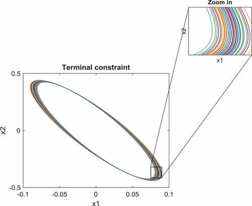
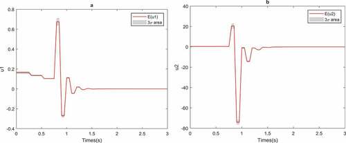
Figure 2 shows how the uncertainty in the parameters of the CSTR affects the optimal control inputs of the system. In other words, it demonstrates how the control input should change to cope with the uncertainty of the parameters in order to have an optimal controller under stable MPC. When the CSTR is exposed to uncertainty, the controls and states will be a stochastic process; thus in Figure 2, the control first and second moments are indicated. The first moment is the mean of the control sequence which is represented by red lines and the gray interval illustrates the three-sigma area, i.e. $\mu \pm 3\sigma$ which is a representation of the second moment. We choose to show the three-sigma area instead of the standard deviation interval $\mu \pm \sigma$ because it can be visualized better in the figures.

Figure 2. Effect of the parameter uncertainty on the control input for CSTR optimal control problem

Based on the three-sigma rule for a Gaussian distributed random variable, the probability of values generated by Gaussian pdf lying in the three-sigma area is 0.9974. We cannot claim that for a nonlinear system, with Gaussian uncertainty parameter distribution, the distribution of the states and the controls of the system remains Gaussian for all time. Generally, with the three-sigma rule, we cannot identify the probability of system inputs but it can visualize the two first moments of the system inputs. Also, by the two first moments, we can apply Markov inequality to characterize the probability of the system states and controls in some bounded domain. Fortunately, in contrast to the three-sigma rule, the Markov inequality is not limited to just Gaussian distribution, it can be used for a wide group of the distributions. To highlight the numerical validation of the proposed method, it is compared with MC simulations. In order to be sure that MC simulations are convergent for our system, we already checked the convergence of MC simulations for both mean and variance of the states and the control of the system with parameter uncertainty under MPC. Figures 3 and 4 demonstrate the comparison between mean and the variance of the states of the system for both MC and gPC uncertainty propagation.

Figure 3. Mean of the optimal states of the CSTR with MC and gPC uncertainty propagation

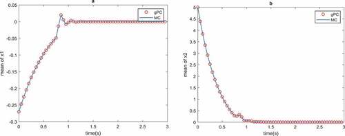
Figure 4. Variance of the optimal states of the CSTR with MC and gPC uncertainty propagation

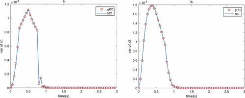
Figures 3 and 4 show that the propose method results are consistent with MC simulations. Also, from Figures 3 and 4, it can be seen that the MPC objective, i.e. stabilization, is satisfied and the states converge to the origin.

The advantage of gPC method compared to MC simulations is the calculation of the mean and the variance of the system with much fewer samples and less computational time. Table 3 compares the computational time and complexity of the gPC and MC simulations for the CSTR tank.

Table 3. Computational time of gPC and MC uncertainty propagation for CSTR optimal control problem

Method	Number of samples	Computational time
gPC	36	11 min
MC	30,000	35 h

Table 3 shows that in order to find the effect of the parameter uncertainty for model predictive control of a CSTR system, 30,000 MC simulations must be performed to have a convergent first and second moment for the states and controls of the system. On the other hand, when gPC is used, only 36 samples are needed to determine the first and second moments of the states and the controls of the CSTR tank. The MPC computational time takes 35 h, whereas gPC method only took 11 min of computational time. Thus, it can be found that gPC is a much more efficient method for uncertainty propagation than the MC simulation method.

Example 2.

In Example 1, the validity of the hPS method has been confirmed for uncertainty propagation when the uncertain parameters both have Gaussian distributions. In this example, the ability of the hPS method will be demonstrated when the uncertain parameters of the system have uniform distributions. Consider the following second-order system with parameter uncertainties A and B:

$\begin{array}{c}{\dot{x}}_1(t)=x_2(t)+B{x}_2(t)\\ {\dot{x}}_2(t)=-(x_1(t)+A{x}_1(t))+u(t)+[1-{(x_1(t)+A{x}_1(t))}^2]((x_2(t)+B{x}_2(t))\end{array}$

The nonlinear dynamic is under MPC strategy with the cost function $l(x,u)=(1/2)(|x{|}_Q^2+|u{|}_R^2)$ with $Q=[10000;01000]$ and $R=[0.00010;00.0001]$, state constraint $-100<x_1,x_2<100$, control constraint $-100<u<100$ and the initial condition $x=[3,3]$. The goal of the MPC is to stabilize the system states to the origin.

The parameter A has uniform distribution $U[-0.01,0.01]$ and parameter B has Weibull distribution $We(B)=\alpha \beta B^{\beta -1}{e}^{-\alpha B^{\beta }}$ with $\alpha =.1$ and $\beta =1$. According to Wiener–Askey scheme for the uniform distribution, the Legendre polynomial should be selected, but no type of polynomial is determined for Weibull distribution. To use Legendre polynomial, fundamental transformation law of probabilities is utilized to map a random variable with uniform distribution to the B as follows: $We(B)={\left[(-1/\alpha )ln(1-b)\right]}^{\frac{1}{\beta }},b=U[0,1]$

Therefore, in the dynamics of the system in the place of B, the term ${\left[(-1/\alpha )ln(1-b)\right]}^{\frac{1}{\beta }}$ should be inserted. We transfer the Weibull distribution to a uniform random distribution to be able to use a type of polynomial according to standard distribution in Wiener–Askey scheme (Table 1). For the terminal constraint we choose ${\mathbb{X}}_f({\theta }_i)=\{x|V_f(x,{\theta }_i)\le 10\}$ and for the linearized feedback controller, ${\kappa }_f(x,{\theta }_i)$ is chosen such that the closed-loop linearized system $A_K({\theta }_i)$ has two stable poles at −2 and −1 for each ${\theta }_i$. For this example, Legendre polynomial for both PS optimal control and gPC uncertainty propagation is applied. The prediction horizon is $N_p=.6s$, control horizon is $N_c=0.1s$, and the system is simulated for 11 s. Also, the number of PS collocation points in the time direction considered to be 4 and $20\times 20=400$ gPC collocation points are considered. Figure 5 highlights how the parameter uncertainty affects the optimal control solution of the system. Figures 6 and 7 indicate the consistency of the gPC method with MC simulations in MPC uncertainty propagation. Also, the MPC objective, i.e. stabilization, is satisfied.

Figure 5. Effect of the parameter uncertainty on the control for optimal control problem of Example 2

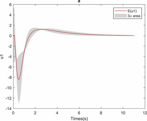
Figure 6. Mean of the optimal states of Example 2 with MC and gPC uncertainty propagation

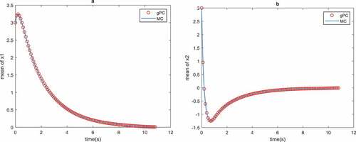
Figure 7. Variance of the optimal states of Example 2 with MC and gPC uncertainty propagation

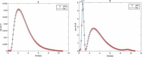
Table 4 compares the computational time and complexity of the gPC and MC simulations for Example 2.

Table 4. Computational time of gPC and MC uncertainty propagation for optimal control problem of Example 2

Method	Number of samples	Computational time
gPC	400	18 min
MC	31,500	27 h

It shows that gPC uncertainty propagation for Example 2 is much more efficient than MC simulations.

Figures 6 and 7 show that gPC results are in consistent with MC simulation results.

7. Conclusion

In this paper, an efficient method is proposed to evaluate the effect of parameter uncertainty on the inputs and the states of a nonlinear dynamical system under the MPC strategy. The presented method implements a hybrid pseudo-spectral method to increase the speed of the process of uncertainty propagation. Based on the proposed method, the first and second moments of the control sequence of a nonlinear system with uncertain parameters have been found. Two simulation results validate the effectiveness of the proposed method. It is shown that the gPC results are consistent with MC simulations, but gPC method is much superior to MC simulations regarding the computational time. In this paper, the hybrid PS method evaluates the first and second moments of the distributions. For future works, the other moments of the distribution can be evaluated by gPC coefficients to have a better analysis of the non-Gaussian distributions.

Additional information

Funding

The authors received no direct funding for this research.

Notes on contributors

Ali Namadchian

Ali Namadchian received the M.Sc. degree in control theory and control engineering from the Islamic Azad University of Mashhad, Mashhad, Iran, in 2013; he is currently pursuing the Ph.D. degree with the Department of Electrical and Control Engineering, Tafresh University, Tafresh, Iran. His current research interests include stochastic control, nonlinear control systems and optimal control.

References

- Annunziato, M., & Borzì, A. (2013). A Fokker–Planck control framework for multidimensional stochastic processes. Journal of Computational and Applied Mathematics, 237, 487–18. doi:10.1016/j.cam.2012.06.019
- Bavdekar, V. A., & Mesbah, A. (2016). Stochastic nonlinear model predictive control with joint chance constraints. IFAC-PapersOnLine, 49, 270–275. doi:10.1016/j.ifacol.2016.10.176
- Becerra, V. M. (2010). Solving complex optimal control problems at no cost with PSOPT. In Computer-Aided Control System Design (CACSD), Yokohama, Japan, 2010 IEEE International Symposium on (pp. 1391–1396.
- Cameron, R. H., & Martin, W. T. (1947). The orthogonal development of non-linear functionals in series of Fourier-Hermite functionals. Annals of Mathematics, 385–392. doi:10.2307/1969178
- Fornberg, B. (1998). A practical guide to pseudospectral methods (Vol. 1). Cambridge: Cambridge university press.
- Garcia, C. E., Prett, D. M., & Morari, M. (1989). Model predictive control: Theory and practice—A survey. Automatica, 25, 335–348. doi:10.1016/0005-1098(89)90002-2
- Gong, Q., Kang, W., Bedrossian, N. S., Fahroo, F., Sekhavat, P., & Bollino, K. (2007). Pseudospectral optimal control for military and industrial applications. In Decision and Control, New Orleans, LA, USA, 2007 46th IEEE Conference on (pp. 4128–4142.
- Gong, Q., Ross, I. M., Kang, W., & Fahroo, F. (2008). Connections between the covector mapping theorem and convergence of pseudospectral methods for optimal control. Computational Optimization and Applications, 41, 307–335. doi:10.1007/s10589-007-9102-4
- Grüne, L., & Pannek, J. (2011). Nonlinear model predictive control (pp. 43–66). London: Springer. ed.
- Harmon, F. G. (2017). Hybrid solution of nonlinear stochastic optimal control problems using Legendre Pseudospectral and generalized polynomial chaos algorithms. American Control Conference (ACC), 2017, 2642–2647.
- Mahmood, M., & Mhaskar, P. (2012). Lyapunov-based model predictive control of stochastic nonlinear systems. Automatica, 48, 2271–2276. doi:10.1016/j.automatica.2012.06.033
- Matsuno, Y., Tsuchiya, T., & Matayoshi, N. (2015). Near-optimal control for aircraft conflict resolution in the presence of uncertainty. Journal of Guidance, Control, and Dynamics, 39, 326–338. doi:10.2514/1.G001227
- Matsuno, Y., Tsuchiya, T., Wei, J., Hwang, I., & Matayoshi, N. (2015). Stochastic optimal control for aircraft conflict resolution under wind uncertainty. Aerospace Science and Technology, 43, 77–88. doi:10.1016/j.ast.2015.02.018
- Mayne, D. Q., Kerrigan, E. C., Van Wyk, E., & Falugi, P. (2011). Tube‐based robust nonlinear model predictive control. International Journal of Robust and Nonlinear Control, 21, 1341–1353. doi:10.1002/rnc.v21.11
- Mayne, D. Q., Rawlings, J. B., Rao, C. V., & Scokaert, P. O. (2000). Constrained model predictive control: Stability and optimality. Automatica, 36, 789–814. doi:10.1016/S0005-1098(99)00214-9
- Muske, K. R., & Rawlings, J. B. (1993). Model predictive control with linear models. AIChE Journal, 39, 262–287. doi:10.1002/(ISSN)1547-5905
- Namadchian, A., & Ramezani, M. (2017). Pseudo-spectral model predictive control of continuous stirred-tank reactor. Majlesi Journal of Mechatronic Systems, 6, 23–28.
- Patterson, M. A., & Rao, A. V. (2014). GPOPS-II: A MATLAB software for solving multiple-phase optimal control problems using hp-adaptive Gaussian quadrature collocation methods and sparse nonlinear programming. ACM Transactions on Mathematical Software (TOMS), 41, 1. doi:10.1145/2684421
- Rawlings, J., & Mayne, D. (2012). Postface to model predictive control: Theory and design. Nob Hill Pub, 5, 155–158.
- Ross, I. M. (2005). A historical introduction to the convector mapping principle. Proceedings of Astrodynamics Specialists Conference. Naval Postgraduate School (U.S.)
- Schwickart, T., Voos, H., Hadji‐Minaglou, J. R., & Darouach, M. (2016). A fast model‐predictive speed controller for minimised charge consumption of electric vehicles. Asian Journal of Control, 18, 133–149. doi:10.1002/asjc.1251
- Visintini, A. L., Glover, W., Lygeros, J., & Maciejowski, J. (2006). Monte Carlo optimization for conflict resolution in air traffic control. IEEE Transactions on Intelligent Transportation Systems, 7, 470–482. doi:10.1109/TITS.2006.883108
- Von Stryk, O., & Bulirsch, R. (1992). Direct and indirect methods for trajectory optimization. Annals of Operations Research, 37, 357–373. doi:10.1007/BF02071065
- Widd, A., Liao, H. H., Gerdes, J. C., Tunestål, P., & Johansson, R. (2014). Hybrid model predictive control of exhaust recompression HCCI. Asian Journal of Control, 16, 370–381.
- Wiener, N. (1938). The homogeneous chaos. American Journal of Mathematics, 60, 897–936. doi:10.2307/2371268
- Xiu, D., & Karniadakis, G. E. (2002). The Wiener–Askey polynomial chaos for stochastic differential equations. SIAM Journal on Scientific Computing, 24, 619–644. doi:10.1137/S1064827501387826