Dynamic performance of a Skystream wind turbine: A bond graph approach

Abstract

The modelling in bond graph of a Skystream wind turbine composed by the blades, a permanent magnet synchronous generator (PMSG), three-phase rectifier, Boost converter and an inverter which is classified as a small-scale system is presented. Bond graphs permit to model systems formed by different energy domains. The Skystream turbine is a good case study to show that the bond graph model is presented in a unified representation approach. The electric power generation system based on this turbine is three-phase, the use of multibond graphs to model the PMSG, three-phase rectifier and inverter are proposed. However, the blades and Boost converter are modelled by single bond graphs. The mathematical representation of a section of a blade and the PMSG are obtained. In order to validate the simulation results obtained by bond graph models, an experimental study of the Skystream is compared with the complete simulation of the turbine. The motivation to develop these models in a bond graph approach is to design and build a low-cost wind turbine similar to the Skystream. Thus, the main contributions of this paper are: a bond graph model of the Skystream wind turbine, the PMSG, rectifier and inverter is modelled by multibond graphs.

Keywords:

• bond graph
• Skystream
• blades
• PMSG
• Recti.er
• boost converter
• inverter

PUBLIC INTEREST STATEMENT

Sustainable electrical energy is a major concern of modern society. Wind power represents a renewable which can be made available on a small-scale system (power below 100 kW) determining a viable solution for energy demand of small urban areas. A commercial wind turbine of this type is Skystream. In this paper, a bond graph model of the Skystream is presented. Bond graph theory is an energy-based modelling approach applied to di§erent physical domains. The motivation to develop this model in a bond graph approach is to design and build a low-cost wind turbine.

1. Introduction

During the last years, wind energy has become one of the most used renewable energies to generate electricity. Actually, the amount of electrical energy generated from wind energy has increased greatly. Hence, the economic utilization of wind resources requires the wind turbines to be connected at remote sites with high average wind speed.

There are many references related to modeling, analysis and control of wind turbines and the following papers can be cited. The modeling of wind turbines for power system studies is investigated in (Petru & Thiringer, 2002; Slootweg, Polinder, & Kling, 2001). The effect of small-scale variable-speed wind energy integration into the local power control is investigated in (Ullah, 2005). The transient stability analysis of wind generator systems by using the equivalent lump mass method is proposed in (Li & Chen, 2007). A complex airfoil wind turbine is proposed in (Li et al., 2019) for a special shape design to combine the horizontal and vertical blades which can deal with the different directions of the wind.

An aggregated model of wind farms with doubly fed induction generators (DFIGs) wind turbines is presented in (Fernandez, Garcia, & Jurado, 2005) by an equivalent wind turbine of aggregated wind turbines under different incoming winds. Modeling and simulation of a grid-connected wind-driven electricity generation system has been done in (Nath, Rana, & Modeling, 2011). A functional structure of a wind energy conversion system is introduced in (Ofualagba & Ubeku, 2008), before making a comparison between the two typical wind turbine operating schemes in operation, namely constant-speed wind turbine and variable-speed wind turbine. A novel isolated small wind turbine emulator for small wind turbine system is described in (Arifujjaman, Iqbal, & Quaicoe, 2006). An energy demand model by designing a hybrid solar-wind-thermal power generation system of the Turkish Republic of Northern Cyprus, a promising substitute for the expensive battery banks is presented in (Aumadu-Sarkodie, Sevinc, & Jayaweera, 2016). A hybrid renewable energy source consisting of solar photovoltaic, wind energy system, and a microhydro system is proposed in (Mosobi, Chichi, & Gao, 2015).

A wind turbine emulator has been developed in (Chinchilla, Arnaltes, & Rodriguez-Amenedo, 2004) to be used in research activities of wind turbine control. The real-time performance of a laboratory-scale model of wind turbine emulator is developed in (Ajewole, Alawode, Omoigui, & Oyekanmi, 2017). A method to simulate wind turbine which includes the calculation method of the torque-speed curve from the rated parameter of actual wind turbine and the implementation of the wind turbine simulator is presented in (Jia, Wang, & Yang, 2007). A nonlinear controller has been designed for variable-speed turbines electric power regulation in (Boukhezzar & Siguerdidjane, 2005). A control of a DFIG based on wind energy power system is investigated in (Alrifai, Zribi, & Rayan, 2016). The dynamic modelling of a hybrid energy system based on an anion exchange membrane fuel cell (AEMFC) is presented in (Frangiacomo et al., 2017). In addition to the two power sources, AEMFC and battery pack, there is a DC-DC buck converter interjected between them. A proposed system PV/Wind/Fuel cell/Battery is connected to a common bus where different loads are connected and unified power quality conditioner (UPQC) is integrated with the microgrid and grid to compensate PQ related problem is analyzed in (Samal & Hota, 2017).

In (Akinrinde, Swanson, & Tiako, 2019), the dynamic performance of different configurations for wind turbine generator under ferroresonant conditions of energization and de-energization is developed. An adaptive robust sliding mode control for a PMSG wind turbine is proposed in (Lee & Chun, 2019). Electromechanical and electromagnetic transient models of a DFIG wind turbine system that consider the interaction of multiple timescale dynamic processes are presented in (Han, Zhang, Wang, Zhang, & Lin, 2018).

The wind turbines are classified by utility-scale systems (power above 1 MW), medium-scale systems (power between 100 kW and 1 MW), small-scale systems (power below 100 kW) and micro-scale systems (power below 1 kW). Small capacity wind turbines can give a viable solution for energy demand of small urban or rural areas (Palmieri et al., 2018). Hence, this paper proposes a bond graph model of a Skystream wind turbine of a capacity of 2.4 kW, and the electrical system is considered as small-scale system. The dynamic performance model of a 2.4 kW Skystream 3.7 has been considered in the study for wind power estimation in (Prajwal & Venayagamoorthy, 2013).

There are two types of generators used in wind energy conversion systems which are doubly fed induction generator (DFIG) and permanent magnet synchronous generator (PMSG). Some advantages can be cited for PMSG: gearbox and excitation current are not required, it is a direct drive type generator and it has good performance. Some relevant papers using PMSG in electrical systems are the following: In (Aliprantis, Papathanassiou, Papadopoulos, & Kladas, 2004), the operation of a variable-speed, stall-regulated wind turbine equipped with a PMSG is examined. In (Chen et al., 2012; Rathod, Jhala, & Patel, 2014), the modeling of a variable-speed wind turbine equipped with a permanent magnet synchronous generator has been described. In (Elbeji, Hamed, & Sbita, 2014), a model of a variable-speed wind turbine using a PMSG is presented and the control schemes are proposed. A five-level full-bridge zero-voltage and zero-current switching DC-DC converter scheme in which all the main switches are operating under soft switching is proposed in (Prasad, Obulesh, & Babu, 2016).),Nonlinear control of permanent magnet synchronous generators using feedback linearization is presented in (Merzoug, Benalla, & Louze, 2011). A control scheme with adaptive gains for a PMSG applied to wind power plant is proposed in (Dai, Tang, & Yi, 2019). Complete and reduced models of wind turbine systems with PMSG are presented in (Hackl, Jane-Soneira, Pfeifer, & Schechner, 2018). In addition, a PMSG is used in the Skystream wind turbine system. A novel soft-switched grid-connected current-source inverter topology and an efficient control strategy using switching flow graph theory are proposed in (Pakdel & Jalilzadeh, 2017). A new configuration for cascaded voltage source multilevel inverter based on series connection of improved sub-multilevel inverter module is presented in (Thakre, Mohanty, Kommunkuri, & Chatterjee, 2016).

The bond graph methodology is an energy-based modelling approach, unifying symbology for phenomena from different physical domains. The essential feature of the bond graph approach is the representation of energetic interactions between systems and/or system components by a single line. Also, the use of a bond graph provides a structured approach to system dynamics modeling (Karnopp, Margolis, & Rosenberg, 2000).

The ability of the bond graph theory can be illustrated with the following papers: A bond graph representation of model-based observer control, which provides a convenient framework for the design of controllers in the physical domain is analyzed in (Gawthrop, 1995). A bond graph model to enable testing the PV system performance by computer simulation was developed in (Mezghanni, Amdoulsi, Mami, & Dauphin- Tanguy, 2007). The physical characteristics of the bond graph representation are exploited for the purpose of controller synthesis in (Yeh, 2002). Some structural properties for switching devices modelled by bond graphs are analyzed in (Rahmani & Dauphin-Tanguy, 2006). The formulation of state, output equations and solutions of switched-systems are presented in (Poyraz, Demir, Gulten, & Koksal, 1999) using the bond graph model with a new simple and more general switch definition. A bond graph approach is proposed in (Delgado & Ramirez, 1998) for the modeling and simulation of switched DC-to-DC power converters of the boost type, regulated by means of a pulse-width-modulation (PWM) strategy.

Bond graphs have the following attractive features among others: (a) Bond graphs are based on an analogy allowing for a uniform modelling of systems across energy domains. (b) A bond graph model can be constructed in a systematic manner from a system schematic. (c) A bond graph can provide a lot of information about a mathematical model to be derived from the graph before any equations are written and reformulated. Moreover, the structural properties of the model (structural controllability, observability, stability, steady state, linearization) can be analyzed directly on a bond graph.

Some of the problems or disadvantages that bond graph has in scientific research are: (a) The methodology is known but it is not easy for the scientific community to understand complicated bond graphs; (b) It is necessary to have some experience to avoid problems with the causality of the elements, for example, algebraic loops and derivative causality; (c) The causality assignment for simple systems may have problems and sometimes it is necessary to introduce some non-modelled dynamics, for example, rectifiers; (d) Some typical control system problems do not have a simple bond graph representation, for example, controllable canonical form; (e) Some typical control problems are open problems, for example, nonlinear control, robust control, etc., and they have not been solved in a bond graph approach.

Some of the first papers of modelling electrical machines in bond graph are: In (Sahm, 1979) the d-q model of the synchronous machine is shown in a bond graph. The feasibility of an induction motor model using a bond graph, representing the magnetic circuit, is shown in (Gaude, Morel, Allard, Yahoui, & Masson, 1998).

Several papers have been published on the modelling of wind turbines using the bond graph methodology. A bond graph model of a blade considering the blade as a Rayleigh beam composed of a number of sections is proposed in (Agarwal, Chalal, Dauphin-Tanguy, & Guillaud, 2012). A non-linear model that describes the wind turbine system taking account of the flexibility of the blades, drive train and tour using bond graph method is described in (Lakhal et al., 2015). The modelling and simulation of wind turbine driven by induction generator is dealt with in (Ramdane, Lachouri, & Krikeb, 2015). A nonlinear model of a wind turbine generating system, containing blade pitch, drive train, tower motion and generator using the bond graph method is presented in (Bakka & Karimi, 2013). A wind turbine composed by blades, gearbox and the induction generator using the bond graph methodology is proposed in (Sanchez & Medina, 2014). A bond graph modeling and a new control scheme of a three-phase grid-connected wind energy conversion system are described in (Badoud, Khemliche, & Chermat, 2013). A detailed bond graph model of a single wind turbine, taking into account the flexibility of the wind turbine blades is presented in (Barrera, Dauphin-Tanguy, & Guillaud, 2015).

Skystream developed by Southwest Windpower in collaboration with U. S. Department of Energy´s National Renewable Energy Laboratory is the newest generation in residential with technology. Skystream has a 2.4 kW rating and is the first fully integrated small wind generator specifically designed for the utility-connected market (Skystream, 2013).

In this paper, a bond graph model of the Skystream wind turbine is presented. The different submodels of this turbine (blades, PMSG, rectifier, boost converter, inverter) are modelled in the physical domain. A junction structure to get the mathematical model of the PMSG multibond graph model is proposed.

The references (Agarwal et al., 2012, Lakhal et al., 2015) give emphasis to obtain the bond graph model of the wind turbine blades and (Bakka & Karimi, 2013; Ramdane et al., 2015; Sanchez & Medina, 2014) construct the bond graph model of the wind turbine system considering an induction generator. This proposed paper builds the bond graph of the system with a PMSG having differences with the published papers. The reference (Badoud et al., 2013) describes the modelling of the system with PMSG with an IGBT converter and inverter. However, the bond graph models do not show in a clear way the electromechanical relations of the PMSG, and the mathematical model is not obtained.

A basic bond graph model of a Skystream wind turbine is proposed in (Gonzalez & Lopez, 2017). Also, a reduced model of a permanent magnet synchronous generator in a bond graph approach is introduced in (Gonzalez, Lopez, & Quasi, 2018).

Thus, this paper constructs a PMSG multibond graph model and the mathematical representation is verified with the published papers (Aliprantis et al., 2004; Chen et al., 2012; Elbeji et al., 2014; Merzoug et al., 2011; Rathod et al., 2014). Also, the power electronics of the Skystream wind turbine (rectifier, converter, inverter) are modelled in a bond graph approach and these devices are simulated. The rectifier and inverter models are built by using multibond graphs. Finally, the complete system is simulated. These simulation results of the complete system are compared with respect to the experimental results given by Skyview software for the Skystream wind turbine.

The contributions of this paper are: (a) A bond graph model of the blades of a Skystream wind turbine; (b) A multibond graph of a PMSG connected to a three-phase supply voltage (a,b,c); (c) A three-phase rectifier modelled by multibond graphs; (d) A three-phase inverter modelled by multibond graphs.

The motivation to model and simulate this wind turbine system is to design and build a similar low-cost wind turbine. Also, some well-known bond graphs structural properties (controllability, observability, steady state) can be extended to multibond graphs for new developments.

Section 2 describes the traditional approach for a Skystream wind turbine. The modelling in bond graph and multibond graph is described in Section 3. In Section 4, the Skytream wind turbine in a bond graph approach is presented. Simulation results of each component and the complete system are shown in Section 5. The experimental and simulation results of the Skystream are compared in Section 6. Finally, Section 7 gives our conclusions.

2. System description

A general scheme of a wind energy conversion system is shown in Figure 1. This system is based on a permanent magnet synchronous generator (PMSG) considering the blades, and electrical and electronic subsystems formed by a rectifier, boost converter and an inverter.

Figure 1. Wind energy conversion system

2.1. Aerodynamic part

The time-average mechanical input power P_m at the shaft of the generator can be calculated from

(1) $P_m=0.5\rho A{V}_w^3{C}_p$(1)

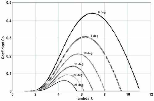
where $\rho =1.15kg/m^3$ denotes air density, A = πR² is the area of the rotor, V_w is the wind velocity and C_p is the aerodynamic power coefficient. The coefficient C_p is a function of the tip speed ratio λ and the pitch angle θ_p and is given by (Aliprantis et al., 2004)

(2) $C_p=0.73{\lambda }_i{e}^{\frac{-18.4}{{\lambda }_{ii}}}$(2)

where

(3) ${\lambda }_i=\frac{151}{{\lambda }_{ii}}-0.58{\theta }_p-0.002\theta {}_p^{2.14}-13.2$(3)

(4) $\frac{1}{{\lambda }_{ii}}=\frac{1}{\lambda -0.02{\theta }_p}-\frac{0.003}{{\theta }_p^3+1}$(4)

By substituting (2), (3) and (4) into block diagrams of 20-SIM software, this leads to the C_p versus λ characteristics for various values of θ_p, as depicted in Figure 2.

Figure 2. Coefficient C_p versus λ

2.2. PMSG model

The Permanent Magnet Synchronous Generator (PMSG) is the electromechanical conversion system used in the Skystream wind turbine. Figure 3 shows the schematic of the cross-section of a three-phase PMSG with one pair of field poles. The model of PMSG has been developed using the following assumptions (Kulkarni & Thosar, 2013): (a) The magnetic saturation effects are neglected; (b) The induced EMT is sinusoidal; (c) Eddy currents and hysteresis losses are negligible; (d) There are no field current dynamics.

Figure 3. PMSG scheme

A great simplification in the mathematical description of a PMSG is obtained from the Park transformation. The effect of the Park transformation is simply to transform all stator quantities from phases a, b, and c into new variables, the frame of reference of which moves with the rotor (Anderson, 1977). Thus, by definition

(5) $\left[\begin{array}{c}{i}_d\\ i_q\\ i_0\end{array}\right]=\sqrt{\frac{2}{3}}\left[\begin{array}{ccc}cos\theta & cos\left(\theta -\frac{2\pi }{3}\right)& cos\left(\theta +\frac{2\pi }{3}\right)\\ \mathrm{s}\mathrm{i}\mathrm{n}\theta & \mathrm{s}\mathrm{i}\mathrm{n}\left(\theta -\frac{2\pi }{3}\right)& \mathrm{s}\mathrm{i}\mathrm{n}\left(\theta +\frac{2\pi }{3}\right)\\ \frac{1}{\sqrt{2}}& \frac{1}{\sqrt{2}}& \frac{1}{\sqrt{2}}\end{array}\right]\left[\begin{array}{c}{i}_a\\ i_b\\ i_c\end{array}\right]$(5)

The angle between the d-axis and the rotor is given by

(6) $\theta =wt+\frac{\pi }{2}$(6)

where w is the rated angular frequency in rad/s.

Similarly, to transform the voltages and flux linkages,

(7) $v_{dq0}=P{v}_{abc}$(7)

(8) ${\lambda }_{dq0}=P{\lambda }_{abc}$(8)

The voltage equations of the stator on (a,b,c) axis for a PMSG are defined by

(9) $v_{abc}=r_s{i}_{abc}+\frac{d{\lambda }_{abc}}{dt}$(9)

where $v_{abc}$, $i_{abc}$ and ${\lambda }_{abc}$ are the voltages, currents and flux linkages on (a,b,c) axis and $r_s$ is the resistance of the stator.

By applying the Park´s transformation to (9) the voltages are expressed by

(10) $v_{dq0}=r_s{i}_{dq0}+w{\lambda }_{qd0}+\frac{d{\lambda }_{dq0}}{dt}$(10)

where ${\lambda }_{qd0}=\left[\begin{array}{c}-{\lambda }_q\\ {\lambda }_d\\ {\lambda }_0\end{array}\right]$. The flux linkage equations are

(11) ${\lambda }_d=L_d{i}_d+{\psi }_f$(11)

(12) ${\lambda }_q=L_q{i}_q$(12)

where ${\psi }_f$ is the permanent magnet rotor flux and, $L_d$ and $L_q$ are the inductances of the stator on (d,q,0) axis.

Substituting (11) and (12) into (10), the state equation of the PMSG for the electrical currents is defined by (Patil & Mehta, 2014)

(13) $\left[\begin{array}{c}\frac{d{i}_d}{dt}\\ \frac{d{i}_q}{dt}\end{array}\right]=\left[\begin{array}{cc}\frac{-r_s}{L_d}& \frac{L_q}{L_d}w\\ \frac{-L_d}{L_q}w& \frac{-r_s}{L_q}\end{array}\right]\left[\begin{array}{c}{i}_d\\ i_q\end{array}\right]+\left[\begin{array}{c}0\\ \frac{-w{\psi }_f}{L_q}\end{array}\right]+\left[\begin{array}{c}\frac{v_d}{L_d}\\ \frac{v_q}{L_q}\end{array}\right]$(13)

Figure 4 illustrates the circuits involved in the analysis of a PMSG on (d,q) axis according to (13).

Figure 4. Circuits of a PMSG on (d,q) axis

Also, the electromagnetic torque is expressed by

(14) $T_e=\left(\frac{3}{2}\right)\left(\frac{p}{2}\right)\left[{\psi }_f{i}_q+\left(L_d-L_q\right)i_d{i}_q\right]$(14)

and the differential equation for the velocity is

(15) $\frac{dw}{dt}=\frac{1}{J}\left(T_e-T_L\right)-\frac{B_m}{J}w$(15)

2.3. Rectifier

Consider a three-phase diode bridge rectifier as shown in Figure 5. This rectifier has diodes D₁ to D₆, and it is assumed that the impedances of the supply lines are low enough to be neglected. The first diode conducting is obtained from the group of diodes {D₁, D₃, D₅} and is connected by its anode at the highest of the phase voltages in the time considered. The second diode conducting is from the group of diodes {D₂, D₄, D₆} and is connected by its cathode to the lowest of the phase voltages.

Figure 5. Three-phase diode rectifier

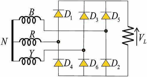
The DC component of the output voltage is defined by

(16) $V_L=\frac{\sqrt{3}}{\pi /3}\underset{\pi /6}{\overset{\pi /2}{\int }}{V}_{m}sin\left(wt+30\right)dwt=\frac{3\sqrt{3}}{\pi }{V}_m$(16)

2.4. Boost converter

A DC-DC converter is an electronic circuit which converts a direct current source from one voltage level to another. DC-DC converters are the power supply that output a fixed voltage efficiently, converting the input voltage. A current-mode controlled DC-DC boost converter is shown in Figure 6 (Radhika, Swathi, & Syed, 2016).

Figure 6. Boost converter

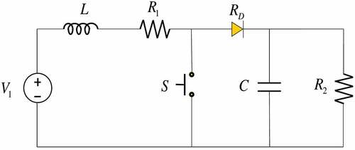
The basic principle of a Boost converter consists of two states: (1) During the ON period of the Switch result in increase in the inductor current; (2) During the OFF period of the Switch the inductor current flows through the diode and the parallel connection of the capacitor, C and resistor, R₂. During the On-state, the switch S is closed which causes the input voltage V₁ to appear through the inductor by changing the current I_L by

(17) $\frac{\mathrm{\Delta }{I}_L}{\mathrm{\Delta }t}=\frac{V_1}{L}$(17)

and the final equation of the two modes is

(18) $\frac{V_0}{V_1}=\frac{1}{1-D}$(18)

where D is the duty cycle.

It can be seen that the output voltage is always greater than the input voltage.

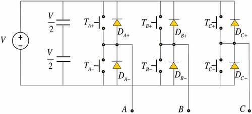
2.5. Inverter

An inverter is a DC to AC converter. It is possible to obtain a single-phase voltage or a three-phase voltage from such a device, but in this paper, only the modelling of a three-phase inverter is described. Figure 7 shows an inverter circuit (Nagaraju & Prakash, 2011). The input to switch-mode inverters is assumed to be a DC voltage source. The inverter must control the magnitude and the frequency of the AC output voltages. This is achieved by PWM of the inverter switches.

Figure 7. Inverter circuit

The basic elements of a typical wind system which is representative of a Sksytream wind turbine have been described.

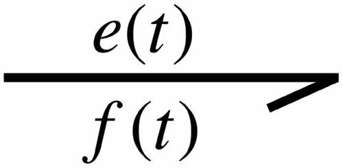
3. Modelling in bond graph

A bond graph model is a graphical representation of a system where the power interactions are described by lines called bonds. These bonds indicate the interactions between power variable pairs called effort e(t) and flow f(t) where the product of effort and flow represents the power which is shown in Figure 8.

Figure 8. A bond

In order to obtain the sets of equations of a system modelled by bond graphs, the constitutive relationships of the elements are required. These relationships can be dynamic or algebraic depending on the element and by the cause-effect assignment. In bond graph, a bond with the causal stroke determines the causality assignment and the assignments of the half arrow and the causal stroke are independent as is shown in Figure 9.

Figure 9. Causal bond

The following physical elements can be used to build a dynamic system:

• The active 1-ports, or sources denoted by (MSe, MSf). These sources have only a causality, this is shown in Figure 10.

• The passive 1-ports, these elements are as follows:

  • Resistance taking whatever causality is shown in Figure 11.

  • Capacitance and inertance elements in an integral causality assignment where the input variable is integrated to produce the output variable which is shown in Figure 12.

  • Capacitance and inertance in a derivative causality assignment where the input and output have a derivative operation and this is shown in Figure 13.

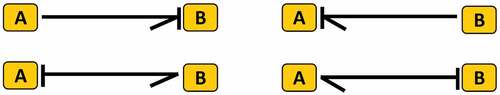
• The ideal 2-port elements denoted by (TF, GY) representing transformers and gyrators, Figure 14 shows these elements.

• The 3-port junctions denoted by (1,0) which are junctions that determine the different connections between the elements, these junctions are shown in Figure 15.

A scheme of a class of non-linear systems modelled by a bond graph is shown in Figure 16.

Figure 10. Power sources

Figure 11. Bond with resistance

Figure 12. Bond in integral causality for capacitance and inertance

Figure 13. Bond in derivative causality for capacitance and inertance

Figure 14. Bonds for transformers and gyrators

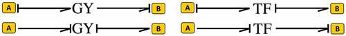
Figure 15. 1 and 0 junctions

Figure 16. Scheme of a bond graph

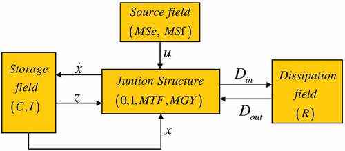
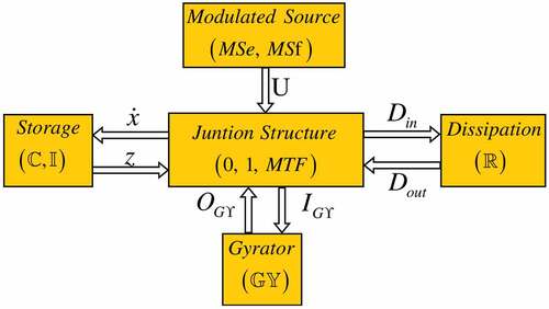
In Figure 16, (MSe,MSf), (C,I) and (R) denote the sources, the energy storage and the energy dissipation fields, respectively, and (0,1,MTF,MGY) the junction structure with transformers MTF and gyrators MGY.

The state $x\left(t\right)\in {\mathrm{\Re }}^n$ is composed of energy variables p(t) and q(t) associated with I and C elements in integral causality assignment, $u\left(t\right)\in {\mathrm{\Re }}^p$ denotes the system input, $z\left(t\right)\in {\mathrm{\Re }}^n$ the co-energy vector and $D_{in}\left(t\right)\in {\mathrm{\Re }}^r$ and $D_{out}\left(t\right)\in {\mathrm{\Re }}^r$ are a mixture of e(t) and f(t) showing the energy exchanges between the dissipation field and the junction structure.

The junction structure of the bond graph model of Figure 16 is given by

(19) $\left[\begin{array}{c}\stackrel{\bullet }{x}\left(t\right)\\ D_{in}\left(t\right)\end{array}\right]=\left[\begin{array}{ccc}{S}_{11}\left(x\right)& S_{12}\left(x\right)& S_{13}\left(x\right)\\ S_{21}\left(x\right)& S_{22}\left(x\right)& S_{23}\left(x\right)\end{array}\right]\left[\begin{array}{c}z\left(t\right)\\ D_{out}\left(t\right)\\ u\left(t\right)\end{array}\right]$(19)

where the entries of S(x) take values inside the set {0, ±1, ±k_t, ±k_g} being k_t and k_g are the transformer and gyrator modules and in the general case can be state variables.

The relationships of the storage and dissipation fields are expressed by

(20) $x\left(t\right)=F^{-1}z\left(t\right)+x_0$(20)

(21) $D_{out}\left(t\right)=L{D}_{in}\left(t\right)$(21)

where F and L are the constitutive relationships of the storage and dissipation elements, respectively, and x₀ is the initial condition of x(t).

From the second line of (19) with (21)

(22) $D_{in}\left(t\right)={\left[I-S_{22}\left(x\right)L\right]}^{-1}\left[S_{21}\left(x\right)z\left(t\right)+S_{23}\left(x\right)u\left(t\right)\right]$(22)

and substituting (22) into the first line of (19)

(23) $\stackrel{\bullet }{x}\left(t\right)=S_{11}\left(x\right)z\left(t\right)+S_{12}\left(x\right)L{\left[I-S_{22}\left(x\right)L\right]}^{-1}\left[S_{21}\left(x\right)z\left(t\right)+S_{23}\left(x\right)u\left(t\right)\right]+S_{13}\left(x\right)u\left(t\right)$(23)

A state space representation for this class non-linear systems modelled by bond graphs is described by

(24) $\stackrel{\bullet }{x}\left(t\right)=A\left(x\right)x\left(t\right)+B\left(x\right)u\left(t\right)$(24)

where

(25) $A\left(x\right)=\left[S_{11}\left(x\right)+S_{12}\left(x\right)M\left(x\right)S_{21}\left(x\right)\right]F$(25)

(26) $B\left(x\right)=S_{13}\left(x\right)+S_{12}\left(x\right)M\left(x\right)S_{23}\left(x\right)$(26)

with

(27) $M\left(x\right)=L{\left[I-S_{22}\left(x\right)L\right]}^{-1}$(27)

A multiport element may store energy or dissipate energy. Analogous to the storage of electrical energy and charge in an ideal electrical capacitor, the energetic multiport element will be called multiport capacitor. Also, analogous to an isothermal electrical resistor, the isothermal entropic, non-energetic, power discontinuous (dissipation of free energy) multiport element will be called multiport resistor. Power and flow discontinuous multiport element is called multiport source, which is a collection of 1-port sources. According to the current bond graph terminology, all non-energetic, power continuous, non-entropic multiport elements belong to a multiport element called generalized junction structure (Breedveld, 1985; Tiernego & Bos, 1985).

Efforts e(t) and flows f(t) in a multibond graph are usually written above or below, to the left or to right of the corresponding multibond, respectively, Although this representation has been called a vector bond notation, it is not a vector but merely a composition of the three bonds, corresponding to the three perpendicular axes, in one multibond. The equivalent bond graph representations as shown in Figure 17 (Breedveld, 1985; Tiernego & Bos, 1985).

Figure 17. Representation of the bonds; (a) Single bond; (b) Multibond

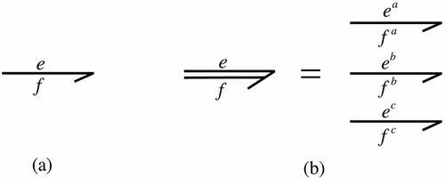
The power flow is now defined as $P\left(t\right)={\underset{\_}{e}}^T\left(t\right)\underset{\_}{f}\left(t\right)$, where ${\underset{\_}{e}}^T\left(t\right)$ is the transpose of the column vector.

$\underset{\_}{e}\left(t\right)=\left[\begin{array}{c}{e}^a\left(t\right)\\ e^b\left(t\right)\\ e^c\left(t\right)\end{array}\right]$ and $\underset{\_}{f}\left(t\right)=\left[\begin{array}{l}{f}^a\left(t\right)\\ f^b\left(t\right)\\ f^c\left(t\right)\end{array}\right]$

A simple multibond graph indicating the variables is shown in Figure 18 (Breedveld, 1985).

Figure 18. Multibond graph with efforts and flows

Multibond graph notation for single port elements (MSe, MSf, I, C, R) is shown in Figure 19.

Figure 19. Multibond graph elements

A special emphasis to consider multiport gyrators is done in this paper whose constitutive relation for a multiport gyrator shown in Figure 20 is (Breedveld, 1985)

Figure 20. Eulerian junction structure

$\begin{array}{rl}& \left(t\right)=\left[\begin{array}{c}{M}_1\left(t\right)\\ M_2\left(t\right)\\ M_3\left(t\right)\end{array}\right]=X\left(Jw\right)\left(t\right)\\ & =\left[\begin{array}{ccc}0& J_3{w}_3\left(t\right)& -J_2{w}_2\left(t\right)\\ -J_3{w}_3\left(t\right)& 0& J_1{w}_1\left(t\right)\\ J_2{w}_2\left(t\right)& -J_1{w}_1\left(t\right)& 0\end{array}\right]\left[\begin{array}{c}{w}_1\left(t\right)\\ w_2\left(t\right)\\ w_3\left(t\right)\end{array}\right]\end{array}$

A multibond graph can be organized into interconnected blocks (modulated sources, storage block, dissipation block, junction structure). Hence, a scheme of a multiport system represented by a multibond graph in a predefined integral causality assignment and key vectors is shown in Figure 21.

Figure 21. Junction structure and key vectors of a multibond graph

In Figure 21, (MSe,MSf) represent the effort and flow modulated multiport sources, storage block for linear multiport elements is (ℂ, I), dissipation block for linear multiport resistors is ℝ and (0, 1, MTF) are the 0 and 1 junctions and MTF denotes the multiport transformers; the multiport gyrators are defined by GY. The energy variables $\underset{\_}{p}\left(t\right)$ and $\underset{\_}{q}\left(t\right)$ are associated with I and ℂ multiport elements in integral causality assignment that represent the state variables $\underset{\_}{x}\left(t\right)\in {\Re }^{\underset{\_}{n}}$, $\underset{\_}{z}\left(t\right)\in {\Re }^{\underset{\_}{n}}$ is the co-energy vector; $\underset{\_}{u}\left(t\right)\in {\Re }^{\underset{\_}{p}}$ denotes the plant inputs; ${\underset{\_}{I}}_{GY}\left(t\right)\in {\Re }^{\underset{\_}{s}}$ and ${\underset{\_}{O}}_{GY}\left(t\right)\in {\Re }^{\underset{\_}{s}}$ are the inputs and outputs of the multiport gyrators, and ${\underset{\_}{D}}_{in}\left(t\right)\in {\Re }^{\underset{\_}{s}}$ and ${\underset{\_}{D}}_{out}\left(t\right)\in {\Re }^{\underset{\_}{s}}$ denote the relation between the dissipation multiport and the junction structure.

The mathematical model of a multibody system based on a multibond graph is determined by the junction structure:

(28) $\left[\begin{array}{c}\dot{x}\left(t\right)\\ -I_{GY}\left(t\right)\\ -D_{in}\left(t\right)\end{array}\right]=\left[\begin{array}{cccc}{S}_{11}^{11}& S_{11}^{12}& S_{12}^{11}& S_{13}^{11}\\ S_{11}^{21}& S_{11}^{22}& S_{12}^{21}& S_{13}^{21}\\ S_{21}^{11}& S_{21}^{12}& S_{22}& S_{23}\end{array}\right]\left[\begin{array}{c}\underset{\_}{z}\left(t\right)\\ \underset{\_}{O_{GY}}\left(t\right)\\ \underset{\_}{D_{out}}\left(t\right)\\ \underset{\_}{u}\left(t\right)\end{array}\right]$(28)

The entries of S take values inside the set {0, ±I, ±K_t}, where K_t is the transformer module, and the constitutive relations for the multiport elements are

(29) $\underset{\_}{x}\left(t\right)=F^{-1}\underset{\_}{z}\left(t\right)+{\underset{\_}{x}}_0$(29)

(30) $\underset{\_}{O_{GY}}\left(t\right)=X_{GY}\underset{\_}{I_{GY}}\left(t\right)$(30)

(31) $\underset{\_}{D_{out}}\left(t\right)=L\underset{\_}{D_{in}}\left(t\right)$(31)

where F, X_GY and L are the constitutive relationships for the multiport storage elements, multiport gyrators and multiport dissipation elements, respectively, and ${\underset{\_}{x}}_0$ is the initial condition of $\underset{\_}{x}\left(t\right)$.

From the second and third lines of (28) with (30) and (21)

(32) $\underset{\_}{I_{GY}}\left(t\right)={\left(I-S_{11}^{22}{X}_{GY}\right)}^{-1}\left[S_{11}^{21}\underset{\_}{z}\left(t\right)+S_{12}^{21}L\underset{\_}{D_{in}}\left(t\right)+S_{13}^{21}\underset{\_}{u}\left(t\right)\right]$(32)

(33) $\underset{\_}{D_{in}}\left(t\right)={\left(I-S_{22}L\right)}^{-1}\left[S_{21}^{11}\underset{\_}{z}\left(t\right)+S_{21}^{12}{X}_{GY}\underset{\_}{I_{GY}}\left(t\right)+S_{23}\underset{\_}{u}\left(t\right)\right]$(33)

The solution of (32) and (33) are

(34) $\underset{\_}{I_{GY}}\left(t\right)={\left(I-S_{11}^{22}{X}_{GY}-S_{12}^{21}{M}_L{S}_{21}^{12}{X}_{GY}\right)}^{-1}\left[\left(S_{11}^{21}+S_{12}^{21}{M}_L{S}_{21}^{11}\right)\underset{\_}{z}\left(t\right)+\left(S_{13}^{21}+S_{12}^{21}{M}_L{S}_{23}\right)\underset{\_}{u}\left(t\right)\right]$(34)

(35) $\underset{\_}{D_{in}}\left(t\right)={\left(I-S_{22}L-S_{21}^{12}{M}_X{S}_{12}^{21}L\right)}^{-1}\left[\left(S_{21}^{11}+S_{21}^{12}{M}_X{S}_{11}^{21}\right)\underset{\_}{z}\left(t\right)+\left(S_{23}+S_{21}^{12}{M}_L{S}_{13}^{21}\right)\underset{\_}{u}\left(t\right)\right]$(35)

where

(36) ${\mathbf{M}}_L=\mathbf{L}{\left(\mathbf{I}-{\mathbf{S}}_{22}\mathbf{L}\right)}^{-1}$(36)

(37) ${\mathbf{M}}_X={\mathbf{X}}_{GY}{\left(\mathbf{I}-{\mathbf{S}}_{11}^{22}{\mathbf{X}}_{GY}\right)}^{-1}$(37)

By substituting (34) and (35) into the first line (28) with (30) and (21)

(38) $\underset{\_}{\dot{x}}\left(t\right)=S_{11}\underset{\_}{z}\left(t\right)+S_{13}^{11}\underset{\_}{u}\left(t\right)+S_{11}^{12}{Q}_X\left[\left(S_{11}^{21}+S_{12}^{21}{M}_L{S}_{21}^{11}\right)\underset{\_}{z}\left(t\right)+\left(S_{13}^{21}+S_{12}^{21}{M}_L{S}_{23}\right)\underset{\_}{u}\left(t\right)\right]+S_{12}^{11}{Q}_L\left[\left(S_{21}^{11}+S_{21}^{12}{M}_X{S}_{11}^{21}\right)\underset{\_}{z}\left(t\right)+\left(S_{21}^{12}{M}_X{S}_{13}^{21}+S_{23}\right)\underset{\_}{u}\left(t\right)\right]$(38)

where

(39) ${\mathbf{Q}}_X={\mathbf{X}}_{GY}{\left[\mathbf{I}-\left(S_{11}^{22}+S_{12}^{21}{M}_L{S}_{21}^{12}\right){\mathbf{X}}_{GY}\right]}^{-1}$(39)

(40) ${\mathbf{Q}}_L=\mathbf{L}{\left[\mathbf{I}-\left(S_{22}+S_{21}^{12}{\mathbf{M}}_X{S}_{12}^{21}\right)\mathbf{L}\right]}^{-1}$(40)

From (38) and (20), a state equation of a system modelled by multibond graphs is defined by

(41) $\underset{\_}{\dot{x}}\left(t\right)=A\underset{\_}{x}\left(t\right)+B\underset{\_}{u}\left(t\right)$(41)

where

(42) $\mathrm{A}=\left[S_{11}^{11}+S_{11}^{12}{\mathbf{Q}}_X\left(S_{11}^{21}+S_{12}^{21}{\mathbf{M}}_L{S}_{21}^{11}\right)+S_{12}^{11}{\mathbf{Q}}_L\left(S_{21}^{11}+S_{21}^{12}{\mathbf{M}}_X{S}_{11}^{21}\right)\right]\mathbf{F}$(42)

(43) $\mathrm{B}=S_{13}^{11}+S_{11}^{12}{\mathbf{Q}}_X\left(S_{13}^{21}+S_{12}^{21}{\mathbf{M}}_L{\mathbf{S}}_{23}\right)+S_{12}^{11}{\mathbf{Q}}_L\left(S_{23}+S_{21}^{12}{\mathbf{M}}_X{S}_{13}^{21}\right)$(43)

The basic elements of single and multibond graphs including mathematical representations have been described. The class of systems modelled by these bond graphs is nonlinear systems which are common for PMSG. Some references have given the mathematical description from the corresponding single bond graphs (Dauphin-Tanguy, 2000). However, in this paper, a state space representation of a system modelled by multibond graphs is proposed.

4. Skystream wind turbine bond graph model

The different stages of a Skystream wind turbine are modelled in the physical domain in this section.

4.1. Blades bond graph model

The modelling of a blade is based on Euler Bernoulli beam model and Blade Elements Momentum (BEM). The rotary inertia and shear deformation are neglected. Only the aerodynamic force corresponding to the differential rotor torque is applied at the centre of gravity of each section. Hence, the blade is divided by three elements and the total deformation of blade is the sum of deformation of sections shown in Figure 22.

Figure 22. Sections of a blade

The corresponding bond graph of the blade is shown in Figure 23. The designed bond graph model takes into account the deformation of the blade. The axial extension deformation and the Coriolis forces effect are not considered. Also, the self-weight of the turbine blade is neglected. In each section, the forces exerted on a C element of the beam are: elastic forces, damping forces, inertial forces and external forces.

Figure 23. Bond graph of a blade

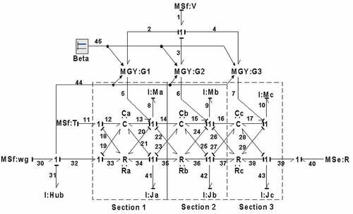
In Figure 23, MSf:V represents the wind velocity; MSf:w_g is the angular velocity of the electrical generator; MSe:R and MSf:T are the boundary conditions for the rotation and translational displacements, respectively; C:C_a, C:C_b and C:C_c are the C-fields denoting the stiffness for each section; R:R_a, R:R_b and R:R_c are the structural damping for each section, I:J_a, I:J_b and I:J_c, and I:M_a, I:M_b and I:M_c are the rotational inertias and mass for each section, respectively, and I:J_hub is the inertia of the rigid body for the hub.

The numerical parameters are determined knowing the length, the number of sections, the inertia and the mass of the blade which are given in Table 1. Also, the power produced by each blade is supplied to the hub and it is considered to be 1/3 of the total power for the wind turbine.

Table 1. Technical specifications (Skystream, 2013)

Rated Capacity	1.8 kW rated 2.4 kW
Weight	77 Kg
Rotor Diameter	3.72 m
Swept Area	10.87 m^2
Type	Downwind rotor with stall regulation control
Direction of Rotation	Clockwise looking upwind
Blade Material	Fiberglass reinforced composite
Number of Blades	3
Rated Speed	50–325 rpm
Tip Speed	9.7–63 m/s
Alternator	Slotless permanent magnet brushless
Yaw Control	Passive
Grid Feeding	120/240 VAC 50–60 Hz
Braking System	Electronic stall regulation
Cut-in Wind Speed	3.5 m/s
Rated Wind Speed	9 m/s
User control	Wireless 2 way interface remote system

The aerodynamic forces acting in each section are represented by gyrators MGY. These gyrators are modulated by the twist angle and the rotational speed of the blade given by

(44) $G_i=\frac{1}{2}\rho v\frac{{\left(1-a_i\right)}^2}{sin{\varphi }_i^2}\left(C_{l}sin{\varphi }_i-C_{d}cos{\varphi }_i\right)c_i{l}_i$(44)

where a_i is the axial induction factor; φ_i is the attack angle of the wind; c_i is the chord distance in the center of gravity; l_i is the length of the blade; C_l is the lift coefficient for a specific airfoil and C_d is the drag coefficient for the same airfoil.

The key vectors of section 1 of the blade are

$x\left(t\right)=\left[\begin{array}{c}{q}_{12}\left(t\right)\\ q_{13}\left(t\right)\\ q_{19}\left(t\right)\\ q_{21}\left(t\right)\\ \begin{array}{c}{p}_3\left(t\right)\\ p_{41}\left(t\right)\end{array}\end{array}\right];\stackrel{\bullet }{x}\left(t\right)=\left[\begin{array}{c}{f}_{12}\left(t\right)\\ f_{13}\left(t\right)\\ f_{19}\left(t\right)\\ f_{21}\left(t\right)\\ \begin{array}{c}{e}_3\left(t\right)\\ e_{41}\left(t\right)\end{array}\end{array}\right];z\left(t\right)=\left[\begin{array}{c}{e}_{12}\left(t\right)\\ e_{13}\left(t\right)\\ e_{19}\left(t\right)\\ e_{21}\left(t\right)\\ \begin{array}{c}{f}_3\left(t\right)\\ f_{41}\left(t\right)\end{array}\end{array}\right]$

$D_{in}\left(t\right)=\left[\begin{array}{c}{e}_{33}\left(t\right)\\ e_{34}\left(t\right)\\ e_{18}\left(t\right)\\ e_{20}\left(t\right)\end{array}\right];D_{out}\left(t\right)=\left[\begin{array}{c}{f}_{33}\left(t\right)\\ f_{34}\left(t\right)\\ f_{18}\left(t\right)\\ f_{20}\left(t\right)\end{array}\right];u\left(t\right)=\left[\begin{array}{c}{f}_1\left(t\right)\\ f_{11}\left(t\right)\\ f_{30}\left(t\right)\\ e_{40}\left(t\right)\end{array}\right];\begin{array}{c}{x}_d\left(t\right)=p_{31}\left(t\right)\\ {\stackrel{\bullet }{x}}_d\left(t\right)=e_{31}\left(t\right)\\ z_d\left(t\right)=f_{31}\left(t\right)\end{array}$

and the constitutive relationships are

(45) $F^{-1}=diag\left\{C_a,M_a,J_a\right\}$(45)

(46) $L=R_a$(46)

where any column of the stiffness matrix can be determined by assigning unit value to the corresponding row element of the displacement vector all elements being zero and then evaluating the equilibrium forces and moments on an element satisfying the following equation to the elastic line:

(47) $M\left(x\right)=EI\frac{{\mathrm{\partial }}^2}{\mathrm{\partial }{x}^2}y\left(x\right)$(47)

In terms of flexural rigidity EI and element length l, the stiffness matrix is given by

(48) $C_a=\frac{EI}{l^3}\left[\begin{array}{cccc}12& 6l& -12& 6l\\ 6l& 4l^2& -6l& 2l^2\\ -12& -6l& 12& -6l\\ 6l& 2l^2& -6l& 4l^2\end{array}\right]$(48)

and the junction structure is described by

(49) $\left[\begin{array}{c}{f}_{12}\\ f_{13}\\ f_{19}\\ f_{21}\\ e_8\\ e_{41}\\ f_{33}\\ f_{34}\\ f_{18}\\ f_{20}\end{array}\right]=\left[\begin{array}{cccccccccccccc}0& 0& 0& 0& 0& 0& 0& 0& 0& 0& 0& 1& 0& 0\\ 0& 0& 0& 0& 1& 0& 0& 0& 0& 0& 0& 0& 0& 0\\ 0& 0& 0& 0& 0& 0& 0& 0& 0& 0& 0& 0& 1& 0\\ 0& 0& 0& 0& 0& 1& 0& 0& 0& 0& 0& 0& 0& 0\\ 0& -1& 0& 0& 0& 0& 0& 0& 0& -1& G_1& 0& 0& 0\\ 0& 0& 0& -1& 0& 0& 0& -1& 0& 0& 0& 0& 0& 1\\ 0& 0& 0& 0& 0& 0& 0& 0& 0& 0& 0& 0& 1& 0\\ 0& 0& 0& 0& 0& 1& 0& 0& 0& 0& 0& 0& 0& 0\\ 0& 0& 0& 0& 0& 0& 0& 0& 0& 0& 0& 1& 0& 0\\ 0& 0& 0& 0& 1& 0& 0& 0& 0& 0& 0& 0& 0& 0\end{array}\right]\left[\begin{array}{c}{e}_{12}\\ e_{13}\\ e_{19}\\ e_{21}\\ f_8\\ f_{41}\\ e_{33}\\ e_{34}\\ e_{18}\\ e_{20}\\ f_1\\ f_{11}\\ f_{30}\\ e_{40}\end{array}\right]$(49)

From (25), (26), (27) with (45) to (49), a state space representation of section 1 of the blade is defined by

(50) $\stackrel{\bullet }{x}\left(t\right)=\left[\begin{array}{cccccc}0& 0& 0& 0& 0& 0\\ 0& 0& 0& 0& 1& 0\\ 0& 0& 0& 0& 0& 0\\ 0& 0& 0& 0& 0& 1\\ 0& -1& 0& 0& -r_{44}& r_{42}\\ 0& 0& 0& -1& -r_{24}& -r_{22}\end{array}\right]x\left(t\right)+\left[\begin{array}{cccc}0& 1& 0& 0\\ 0& 0& 0& 0\\ 0& 0& 1& 0\\ 0& 0& 0& 0\\ G_1& -r_{43}& -r_{41}& 0\\ 0& -r_{23}& -r_{21}& 1\end{array}\right]u\left(t\right)$(50)

Similar results can be obtained for sections 2 and 3 or for the full blade.

4.2. PMSG bond graph model

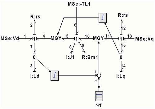
The modelling in bond graph of a PMSG using single bonds on (d,q) axis is shown in Figure 24. The mechanical subsystem is defined by

• MS_e:-T_L1 represents the input torque.

• I:J₁ determines the rotor inertia.

• R:B_m1 describes the mechanical friction.

The electrical subsystem is given by

• MS_e:V_d and MS_e:V_q are the input voltages.

• I:L_d and I:L_q are the inductances.

• R:R_s for the bonds 2 and 12 are resistances.

The conversion of mechanical to electrical energy is obtained by MGY elements modulated by the state variables p₃(t) and p₁₄(t) which are defined by the integral of the efforts of 0-junctions connected to I:L_d and I:L_q elements, respectively. Finally, the permanent magnet rotor flux ψ_f is introduced.

Figure 24. PMSG bond graph

The key vectors of the bond graph is

$\begin{array}{rl}& x\left(t\right)=\left[\begin{array}{c}{p}_3\left(t\right)\\ p_{14}\left(t\right)\\ p_8\left(t\right)\end{array}\right];\stackrel{\bullet }{x}\left(t\right)=\left[\begin{array}{c}{e}_3\left(t\right)\\ e_{14}\left(t\right)\\ e_8\left(t\right)\end{array}\right];z\left(t\right)=\left[\begin{array}{c}{f}_3\left(t\right)\\ f_{14}\left(t\right)\\ f_8\left(t\right)\end{array}\right]\\ \\ & D_{in}\left(t\right)=\left[\begin{array}{c}{f}_2\left(t\right)\\ f_{12}\left(t\right)\\ f_9\left(t\right)\end{array}\right];D_{out}\left(t\right)=\left[\begin{array}{c}{e}_2\left(t\right)\\ e_{12}\left(t\right)\\ e_9\left(t\right)\end{array}\right];u\left(t\right)=\left[\begin{array}{c}{e}_1\left(t\right)\\ e_{13}\left(t\right)\\ e_6\left(t\right)\end{array}\right]\end{array}$

The constitutive relations are

(51) $F^{-1}=diag\left\{L_d,L_q,J_1\right\}$(51)

(52) $L=diag\left\{r_s,r_s,B_{m1}\right\}$(52)

(53) $x_0={\left[\begin{array}{ccc}{\psi }_f& 0& 0\end{array}\right]}^T$(53)

and the junction structure is given by

(54) $\left[\begin{array}{c}{e}_3\left(t\right)\\ e_{14}\left(t\right)\\ e_8\left(t\right)\\ f_2\left(t\right)\\ f_{12}\left(t\right)\\ f_9\left(t\right)\end{array}\right]=\left[\begin{array}{ccccccccc}0& 0& p_{14}\left(t\right)& -1& 0& 0& 1& 0& 0\\ 0& 0& -p_3\left(t\right)& 0& -1& 0& 0& 1& 0\\ -p_{14}\left(t\right)& p_3\left(t\right)& 0& 0& 0& -1& 0& 0& 1\\ 1& 0& 0& 0& 0& 0& 0& 0& 0\\ 0& 1& 0& 0& 0& 0& 0& 0& 0\\ 0& 0& 1& 0& 0& 0& 0& 0& 0\end{array}\right]\left[\begin{array}{c}{f}_3\left(t\right)\\ f_{14}\left(t\right)\\ f_8\left(t\right)\\ e_2\left(t\right)\\ e_{12}\left(t\right)\\ \begin{array}{c}{e}_9\left(t\right)\\ e_1\left(t\right)\\ e_{13}\left(t\right)\\ e_6\left(t\right)\end{array}\end{array}\right]$(54)

Substituting (61), (62), (63) and (54) into (24), (25), (26) with (27), the state equation is

(55) $\left[\begin{array}{c}{e}_3\left(t\right)\\ e_{14}\left(t\right)\\ e_8\left(t\right)\end{array}\right]=\left[\begin{array}{ccc}-r_s& 0& p_{14}\left(t\right)\\ 0& -r_s& -p_3\left(t\right)\\ -p_{14}\left(t\right)& p_{3\left(t\right)}& -B_{m1}\end{array}\right]F\left[\begin{array}{c}{p}_3\left(t\right)\\ p_{14}\left(t\right)\\ p_8\left(t\right)\end{array}\right]+\left[\begin{array}{c}{e}_1\left(t\right)\\ e_{13}\left(t\right)\\ e_6\left(t\right)\end{array}\right]$(55)

Applying the derivative of (20) with (61) and (63)

(56) $\left[\begin{array}{c}{L}_d\frac{d{f}_3\left(t\right)}{dt}\\ L_q\frac{d{f}_{14}\left(t\right)}{dt}\\ J_1\frac{d{f}_8\left(t\right)}{dt}\end{array}\right]=\left[\begin{array}{ccc}-r_s& 0& p_{14}\left(t\right)\\ 0& -r_s& -p_3\left(t\right)\\ -p_{14}\left(t\right)& p_{3\left(t\right)}& -B_{m1}\end{array}\right]\left[\begin{array}{c}{f}_3\left(t\right)\\ f_{14}\left(t\right)\\ f_8\left(t\right)\end{array}\right]+\left[\begin{array}{c}{e}_1\left(t\right)\\ e_{13}\left(t\right)\\ e_6\left(t\right)\end{array}\right]$(56)

Reducing (56) with

(57) $\left[\begin{array}{c}{f}_3\left(t\right)\\ f_{14}\left(t\right)\\ f_{18}\left(t\right)\end{array}\right]=\left[\begin{array}{c}{i}_d\left(t\right)\\ i_q\left(t\right)\\ w\left(t\right)\end{array}\right];\left[\begin{array}{c}{e}_1\left(t\right)\\ e_{13}\left(t\right)\\ e_6\left(t\right)\end{array}\right]=\left[\begin{array}{c}{v}_d\left(t\right)\\ v_1\left(t\right)\\ T_{L1}\left(t\right)\end{array}\right];\begin{array}{c}{p}_{14}\left(t\right)=L_q{i}_q\left(t\right)\\ p_3\left(t\right)=L_d{i}_d\left(t\right)+{\psi }_f\end{array}$(57)

the state variables for the electrical currents are

(58) $\left[\begin{array}{c}{L}_d\frac{d{i}_d\left(t\right)}{dt}\\ L_q\frac{d{i}_q\left(t\right)}{dt}\end{array}\right]=\left[\begin{array}{cc}-r_s& L_{q}w\left(t\right)\\ -L_{d}w\left(t\right)& -r_s\end{array}\right]\left[\begin{array}{c}{i}_d\left(t\right)\\ i_q\left(t\right)\end{array}\right]+\left[\begin{array}{c}0\\ -{\psi }_{f}w\left(t\right)\end{array}\right]+\left[\begin{array}{c}{v}_d\left(t\right)\\ v_q\left(t\right)\end{array}\right]$(58)

It can be seen that the mathematical representation for the PMSG given by (58) is the same as (13).

The electromagnetic torque is obtained from the third line of (56) with (57)

(59) $J_1\frac{dw\left(t\right)}{dt}=T_{e1}\left(t\right)-T_{L1}\left(t\right)-B_{m1}w\left(t\right)$(59)

where

(60) $T_{e1}\left(t\right)={\psi }_f{i}_q\left(t\right)\left(L_d-L_q\right)i_d\left(t\right)i_q\left(t\right)$(60)

In order to obtain (14) and (15), the relationships of the parameters for the angular velocity are $J_1=J/0.75p,B_{m1}=B_m/0.75p,T_{L1}=-T_L/0.75p$.

Now, a multibond graph of the PMSG with Park´s transformation is illustrated in Figure 25.

Figure 25. PMSG multibond graph

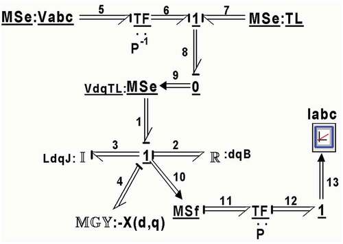
The key vectors of the multibond graph of Figure 25 are described by

$\underset{}{\underset{\_}{x}}\left(t\right)={\underset{-}{p}}_3\left(t\right)=\left[\begin{array}{c}{p}_{3,d}\left(t\right)\\ p_{3,q}\left(t\right)\\ p_{3,J}\left(t\right)\end{array}\right];\stackrel{\bullet }{\underset{-}{x}}\left(t\right)={\underset{-}{e}}_3\left(t\right)=\left[\begin{array}{c}{e}_{3,d}\left(t\right)\\ e_{3,q}\left(t\right)\\ e_{3,J}\left(t\right)\end{array}\right];\underset{}{\underset{\_}{z}}\left(t\right)={\underset{}{\underset{\_}{f}}}_3\left(t\right)=\left[\begin{array}{c}{f}_{3,d}\left(t\right)\\ f_{3,q}\left(t\right)\\ f_{3,J}\left(t\right)\end{array}\right]$

$\underset{\_}{D_{in}}\left(t\right)=-f_2\left(t\right)=\left[\begin{array}{l}{f}_{2,d}\left(t\right)\\ f_{2,q}\left(t\right)\\ f_{2,B}\left(t\right)\end{array}\right];-D_{out}\left(t\right)=-e_2\left(t\right)=\left[\begin{array}{l}{e}_{2,d}\left(t\right)\\ e_{2,q}\left(t\right)\\ e_{2,B}\left(t\right)\end{array}\right];\underset{\_}{u}\left(t\right)={\underset{\_}{e}}_1\left(t\right)=\left[\begin{array}{l}{e}_{1,d}\left(t\right)\\ e_{1,q}\left(t\right)\\ e_{1,T}\left(t\right)\end{array}\right]$

${\underset{}{\underset{\_}{I}}}_{GY}\left(t\right)={\underset{-}{f}}_4\left(t\right)=\left[\begin{array}{c}{f}_{4,d}\left(t\right)\\ f_{4,q}\left(t\right)\\ f_{4,J}\left(t\right)\end{array}\right];{\underset{-}{O}}_{GY}\left(t\right)={\underset{-}{e}}_4\left(t\right)=\left[\begin{array}{c}{e}_{4,d}\left(t\right)\\ e_{4,q}\left(t\right)\\ e_{4,J}\left(t\right)\end{array}\right]$

The constitutive relationships are

(61) $F^{-1}=L_{dqJ}=diag\left\{L_d,L_q,J_1\right\}$(61)

(62) $L=R_{dqB}=diag\left\{r_s,r_s,B_{m1}\right\}$(62)

(63) $x_0={\left[\begin{array}{ccc}{\psi }_f& 0& 0\end{array}\right]}^T$(63)

(64) $X_{GY}=-X\left(d,q\right)=\left[\begin{array}{ccc}0& 0& -p_{3,q}\left(t\right)\\ 0& 0& p_{3,d}\left(t\right)\\ p_{3,q}\left(t\right)& -p_{3,d}\left(t\right)& 0\end{array}\right]$(64)

and the junction structure is given by

(65) $\left[\begin{array}{c}{\underset{}{\underset{\_}{e}}}_3\left(t\right)\\ {\underset{}{\underset{\_}{f}}}_4\left(t\right)\\ {\underset{}{\underset{\_}{f}}}_2\left(t\right)\end{array}\right]=\left[\begin{array}{cccc}0& -I& -I& I\\ I& 0& 0& 0\\ I& 0& 0& 0\end{array}\right]\left[\begin{array}{c}{\underset{}{\underset{\_}{f}}}_3\left(t\right)\\ {\underset{}{\underset{\_}{e}}}_4\left(t\right)\\ {\underset{}{\underset{\_}{e}}}_2\left(t\right)\\ {\underset{}{\underset{\_}{e}}}_1\left(t\right)\end{array}\right]$(65)

By substituting (61), (62), (63), (64) and (65) into (41), (42), (43), (36) with (39), the state equation is

(66) ${\underset{\_}{e}}_3\left(t\right)=-\left[R_{dqB}+X\left(d,q\right)\right]L_{dqJ}-p_3\left(t\right)+-e_1\left(t\right)$(66)

Applying the derivative of (20) with (61) and (63)

(67) $\left[\begin{array}{c}{L}_d\frac{d{f}_3\left(t\right)}{dt}\\ L_q\frac{d{f}_{14}\left(t\right)}{dt}\\ J_1\frac{d{f}_8\left(t\right)}{dt}\end{array}\right]=\left[\begin{array}{ccc}-r_s& 0& p_{3,q}\left(t\right)\\ 0& -r_s& -p_{3,d}\left(t\right)\\ -p_{3,q}\left(t\right)& p_{3,d}\left(t\right)& -B_{m1}\end{array}\right]\left[\begin{array}{c}{f}_3\left(t\right)\\ f_{14}\left(t\right)\\ f_8\left(t\right)\end{array}\right]+\left[\begin{array}{c}{e}_1\left(t\right)\\ e_{13}\left(t\right)\\ e_6\left(t\right)\end{array}\right]$(67)

The third line of (67) determines the torque electromagnetic.

(68) $T_{e1}\left(t\right)=p_3\left(t\right)f_{14}\left(t\right)-p_{14}\left(t\right)f_3\left(t\right)$(68)

Note that a multibond graph of the PMSG is a compact graphical representation and it is easy to include the Park´s transformation.

4.3. Three-phase rectifier

In this section, the diodes are modelled by Hybrid Bond Graph Methodology (HBGM). Hybrid systems are continuous dynamics and discrete events modelled by modes. Hybrid Bond Graph (HBG) is an extension of Bond Graph, it has been applied to model fast switching in solid-state elements: diodes, transistors, Mosfets, etc., which are characterized by a fast dynamic behavior.

HBG is denoted by G(S,Z) which is used to determine the orientation of the flow or effort according to the activation of the set of edges Z (1_SJ or 0_Sk junctions). The controlled 1_SJ-junction enforces zero flow to all connected bonds when it is turned off (S_j = OFF) and the same happens with the controlled 0_Sk-junction, where it forces the effort at all the connected bonds (S_k = OFF). Three-phase bridge rectifiers are commonly used for high power DC applications. The three-phase rectifier for the Skystream turbine is shown in Figure 3 where D₁, D₂, D₃, D₄, D₅ and D₆ are used in order to conduct a sequence of output to the load and generate a conduction angle of each diode which is 2π/3. The relationships between each diode and the output voltage are given by

(69) $\begin{array}{rl}& D_6,D_1\begin{array}{c}\hspace{0.17em}\end{array}if\begin{array}{c}\pi /3\ge wt\le 2\pi /3\Rightarrow V_L=V_{RY}\end{array}\\ & D_1,D_2\begin{array}{c}\hspace{0.17em}\end{array}if2\begin{array}{c}\pi /3\ge wt\le \pi \Rightarrow V_L=V_{RB}\end{array}\\ & D_2,D_3\begin{array}{c}\hspace{0.17em}\end{array}if\begin{array}{c}\pi \ge wt\le 4\pi /3\Rightarrow V_L=V_{YB}\end{array}\\ & D_3,D_4\begin{array}{c}\hspace{0.17em}\end{array}if\begin{array}{c}4\pi /3\ge wt\le 5\pi /3\Rightarrow V_L=V_{YR}\end{array}\\ & D_4,D_5\begin{array}{c}\hspace{0.17em}\end{array}if5\begin{array}{c}\pi /3\ge wt\le 2\pi \Rightarrow V_L=V_{BR}\end{array}\end{array}$(69)

where the voltages V_RY, V_RB, V_YR and V_BR are the line voltages from each point R, Y and B.

Diode Switching dynamics can be modelled with a controlled junction represented by 1_s or X₁ and 0_s or X₀.

Hybrid MultiBond Graph (HMBG) which is denoted as G(S_m,Z_n) determines the orientation of the multi-flow or multi-effort according to the activation of the set of edges Z_n (1_mn or 0_mn) junctions. The controlled 1_mn-junction enforces zero flow to all connected bonds when it is turned off (1_mn = OFF) and the same happens with the controlled 0_mn-junction, where it forces the effort to zero at all the connected bonds (0_mn = OFF).

A multibond graph of the three-phase rectifier of Figure 3 is presented in Figure 26.

Figure 26. HMBG of the rectifier

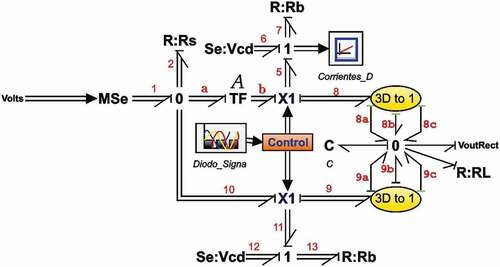
In order to obtain the effort vector $v_a={\left[\begin{array}{ccc}{V}_{BY}& V_{RY}& V_{RB}\end{array}\right]}^T$ from (69) due to the phase voltages $v_b={\left[\begin{array}{ccc}{V}_{BN}& V_{RN}& V_{RN}\end{array}\right]}^T$ a multiport transformer of Figure 26 is applied whose gain matrix is given by

(70) $A^{-1}=\left[\begin{array}{ccc}1& 1& 0\\ 1& 0& 1\\ 0& 1& 1\end{array}\right]$(70)

This model has six elements to control the three-phase voltage supplied to the three-phase bridge rectifier using X₁ junctions according to Equation (69)(69) $\begin{array}{rl}& D_6,D_1\begin{array}{c}\hspace{0.17em}\end{array}if\begin{array}{c}\pi /3\ge wt\le 2\pi /3\Rightarrow V_L=V_{RY}\end{array}\\ & D_1,D_2\begin{array}{c}\hspace{0.17em}\end{array}if2\begin{array}{c}\pi /3\ge wt\le \pi \Rightarrow V_L=V_{RB}\end{array}\\ & D_2,D_3\begin{array}{c}\hspace{0.17em}\end{array}if\begin{array}{c}\pi \ge wt\le 4\pi /3\Rightarrow V_L=V_{YB}\end{array}\\ & D_3,D_4\begin{array}{c}\hspace{0.17em}\end{array}if\begin{array}{c}4\pi /3\ge wt\le 5\pi /3\Rightarrow V_L=V_{YR}\end{array}\\ & D_4,D_5\begin{array}{c}\hspace{0.17em}\end{array}if5\begin{array}{c}\pi /3\ge wt\le 2\pi \Rightarrow V_L=V_{BR}\end{array}\end{array}$(69) . Two blocks represented by 3D to 1 in Figure 26 are used to connect a single 0-junction to the load.

4.4. Boost converter

The modelling in bond graph of the boost converter is shown in Figure 27. Using the circuit of Figure 4, the boost converter is built.

Figure 27. Bond graph model of the boost converter

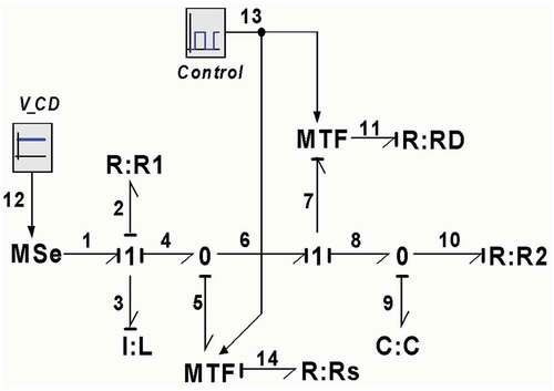
In this section, the different switching elements in the physical domain are modelled by a linear resistance connected to a modulated transformer, which is shown in Figure 28 (Dauphin-Tanguy, 2000).

Figure 28. Switching element models

The element switching feature is that its value changes with the switching command. Figure 28 shows two options to represent the switching elements depending on their causality. In the case of Figure 28(a), the switching command m = 0 indicates closed circuit (conduction) of the element and m = 0 open circuit (not conduction); for Figure 29(b) 1/m = 0 open circuit and 1/m = 1 closed circuit.

4.5. Three-phase inverter

The construction of the multi-level inverter is to create a sine voltage from a voltage level and divided into several stages which is called multi-level. This model is a Hybrid MultiBond graph model of a three-phase five level shown in Figure 29.

Figure 29. Hybrid multibond graph model of a three-phase five level

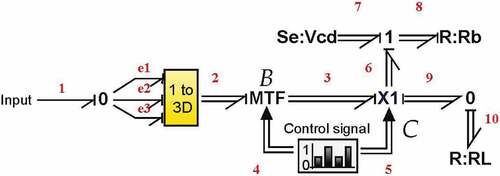
The input voltage is linked to the 0-junction in order to divide into three voltages. Next, a block 1 to 3D is used, this way a multibond is formed by a set of single bonds. Then, the multi-level voltages are transformed through the bond graph element MTF which represents the change of voltages from V_dc to V_dc/2 or -V_dc/2 for each phase to synthesize a sinusoidal output defined by

$\begin{array}{l}\underset{\_}{f_{out}}\left(t\right)=B-f_{in}\left(t\right)\\ \underset{\_}{e_{out}}\left(t\right)=B^{-1}-e_{in}\left(t\right)\end{array}$

This element is an equivalent multiport of the single modulated transformer. The relationship is written as a matrix of 3 × 3 and the ratio M is a set by an input signal from the control signal.

(71) $\left[\begin{array}{c}{v}_a\\ v_b\\ v_c\end{array}\right]={\left[\begin{array}{ccc}{\rho }_a& 0& 0\\ 0& {\rho }_b& 0\\ 0& 0& {\rho }_c\end{array}\right]}^{-1}\left[\begin{array}{c}{e}_1\\ e_2\\ e_3\end{array}\right]$(71)

Equation (71)(71) $\left[\begin{array}{c}{v}_a\\ v_b\\ v_c\end{array}\right]={\left[\begin{array}{ccc}{\rho }_a& 0& 0\\ 0& {\rho }_b& 0\\ 0& 0& {\rho }_c\end{array}\right]}^{-1}\left[\begin{array}{c}{e}_1\\ e_2\\ e_3\end{array}\right]$(71) contains the coefficients that change according to the transition angle of the signal period (ρ_a, ρ_b, ρ_c) the three values form the voltage levels (0, V_dc, 2V_dc, -V_dc, −2V_dc) due to the inverse matrix of a regular diagonal matrix B is a diagonal matrix whose diagonal elements are the inverse of those of B, so the values are 1000, V_dc, 0.5V_dc, -V_dc and −0.5V_dc and the transition is given by

$B_{3\times 3}=\left\{\begin{array}{cc}diag\left[1000,-V_{dc},2V_{dc}\right]& 0\le wt\le \pi /6\\ diag\left[2V_{dc},-V_{dc},1000\right]& \pi /6\le wt\le \pi /3\\ diag\left[V_{dc},-2V_{dc},1000\right]& \pi /3\le wt\le \pi /2\\ ⋮& ⋮\\ diag\left[1000,-2V_{dc},V_{dc}\right]& \pi /6\le wt\le 2\pi \end{array}\right\}$

Finally, at the output of the transformer, a multibond switching the 1-junction is connected depending on the state, it can be connected or disconnected. The bonds 3, 6, 9 are connected when the condition is different to zero. Hence, the sum of the voltages on bonds 3, 6 and 9 is zero and the current on all bonds connected are equal when condition = 1.

$C_{3\times 1}=\left\{\begin{array}{cc}\left[0,1,1\right]& 0\le wt\le \pi /6\\ \left[1,10\right]& \pi /6\le wt\le \pi /3\\ \left[1,10\right]& \pi /3\le wt\le \pi /2\\ ⋮& ⋮\\ \left[0,1,1\right]& \pi /6\le wt\le 2\pi \end{array}\right\}$

The input signal is a matrix 3 × 1 from the control signal switches the output of bond 9, so, the 1X-junction creates the topology of the five-level three-phase cascade hybrid multilevel inverter proposed.

Each element of the Skystream wind turbine has been modelled by single and multibond graphs Note that bond graph methodology allows to unify the representation of different energy domains (mechanical, electrical and electronic). In (Agarwal et al., 2012) the blades of a wind turbine are modelled in bond graphs. In (Ramdane et al., 2015; Sanchez & Medina, 2014), wind systems using induction generators are analyzed in the physical domain. In this paper, the blades connected to a PMSG and the power electronic needed for the Skystream in a bond graph approach are presented. Moreover, the use of multibond graphs in this type of systems is a new contribution of this paper.

5. Simulations

In order to show the effectiveness of the proposed bond graph models, simulation results are depicted. Figure 30 shows the complete system of the Skystream wind turbine. The dynamic behavior of each component is described in the following subsections. 20-SIM software to get the simulations of the different subsystems represented in bond graphs has been used. The numerical parameters for each section of the system are given in Section 6.

Figure 30. Elements of the Skystream wind turbine

5.1. Blades

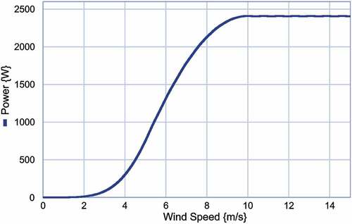
The dynamic performance of the electrical power produced for the Skystream wind turbine at different wind speeds using the bond graph model is shown in Figure 31.

Figure 31. Electrical power of the blades for the Skystream

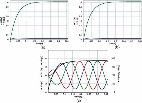
5.2. PMSG results

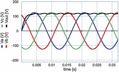
The numerical parameters of the PMSG bond graph model of Figure 25 are the following: r_d = r_q = 3.15 Ω, L_d = L_q = 0.0084 H, J = 0.003192 Nms², B_m = 0.0317 Ns/m and ψ_f = 0.433wb. The voltages and electrical currents on (d,q) axis are shown in Figure 32(a,b), respectively. The angular velocity and electrical currents on axes (a,b,c) are shown in Figure 32(c).

Figure 32. Simulation results of PMSG: (a) Voltages on (d,q) axis; Electrical Currents on (d,q) axis; (c) Velocity and electrical currents on (a,b,c)

5.3. Rectifier results

Figure 33 shows the three-phase voltages supplied to the bond graph model for the rectifier (Figure 26) and the rectifier output, where v_cd = 0.01 V and R_b = 1 Ω.

Figure 33. Simulation results of the rectifier

Note that an almost constant output signal from the rectifier has been obtained.

5.4. Boost converter and inverter results

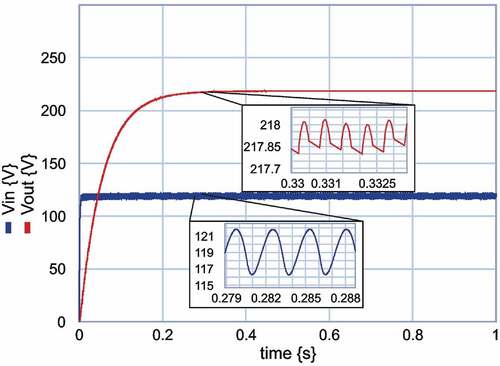
The numerical parameters of the converter are: input voltage, V_DC = 121 V, R₁ = 100 Ω, L = 0.05 H, R₂ = 10 kΩ, C = 0.0015 F, the signal to change the switch and diode conditions is a wave generator-square of magnitude of 1, frequency 100rad/s and the duty cycle is D = 0.5. Figure 34 shows the input and output voltages.

Figure 34. Simulation results of the Boost converter and inverter

Note that the output voltage V_o(DC) ≅1.8 V_i(DC) due to D = 0.5. The boost converter is used to control the magnitude of the output voltage in order to supply a three-phase voltage of 127 V.

5.5. Inverter

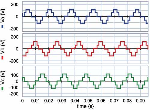
The output voltages of the three-phase inverter are shown in Figure 35. It can be seen that this stage represents three-phase five levels.

Figure 35. Output voltages of the inverter

Thus, the dynamic behavior of each component of the Skystream wind turbine using bond graph models has been illustrated.

6. Experimental study with Skystream

The bond graph models will be validated on the Skystream wind turbine installed at the University of Michoacan. This turbine is shown in Figure 36, and the corresponding components are shown in Figure 31. The wind turbine output is connected to the campus grid. The turbine has been mounted on a 6.5 m tower on a 12 m high building which is shown in Figure 36. The Skystream characteristics are given in Table 1.

Figure 36. Skystream ubicated at the University of Michoacan

The dynamic performance of the Skystream power from the real data and simulation is shown in Figure 37. The real data were obtained from the Skyview, this is the data acquisition software for the Skystream.

Figure 37. Skystream power from real data and simulation

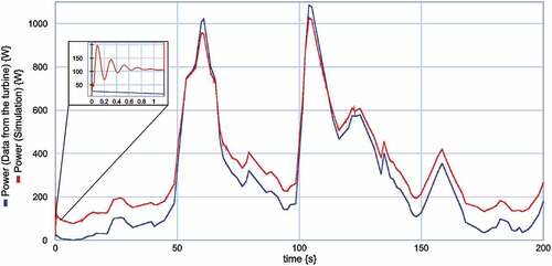
Figure 38. Error analysis: (a) Absolute error; (b) Relative error

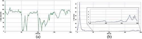
An error analysis of the simulation results respect to real data is shown in Figure 38. The absolute error is calculated by

$Abs\begin{array}{c}\hspace{0.17em}\end{array}error=\left|Powe{r}_{data}-Powe{r}_{simulated}\right|$

and the relative error is given by

$Re\begin{array}{c}\hspace{0.17em}\end{array}error=\frac{Abs\begin{array}{c}\hspace{0.17em}\end{array}error}{Powe{r}_{data}}$

As shown in Figure 38, the simulated power and the real data power can have a significant error due to:

• Geometrical parameters of the blade.

• Numerical parameters of the PMSG.

• Duty cycle of the boost converter.

• Low speed controller.

The different factors described above to reduce the error of the simulation results have to be considered. However, in order to reduce the error, the data sheets of the wind turbine have to be known, and for the Skystream wind turbine, some parameters have been estimated. To include new physical elements or modify bond graph models for each wind turbine component is a simple and straightforward task due to the essence of this graphical approach.

7. Conclusions

The Skystream wind turbine is a system formed by different transformation energy domains: the blades (fluid dynamics-mechanical energies), PMSG (mechanical-electrical energies), rectifier, boost converter and inverter (electrical-electronic energies). Hence, bond graph methodology permits to model these elements of the turbine in a unified approach.

The blades of this turbine are modelled by a single bond graph and the state equation of a blade section is obtained. This is a new result for this particular wind turbine. Also, a new design of the blades of this turbine is a future work where the appropriate parameters can be introduced to the bond graph model, the new blades will be built and installed in the Skystream turbine where the acquisition of real data will be compared with the results of this paper.

The modelling in single bond graph and the mathematical representation of a PMSG were obtained. Also, a multibond graph of this PMSG on (d,q) axes connected to a three-phase supply voltage (a,b,c) is another contribution of this paper. The simulation results for other PMSG can be obtained by replacing the appropriate numerical parameters of the system and is applicable in other similar PMSG connected to an electrical power system.

The multibond graph for the rectifier is a new contribution. In <cite>Les</cite> describes the different elements of the power electronics in bond graphs. This paper proposes to use the hybrid bond graphs for multibond graphs. The 3-phase inverter applied to the wind turbine system modelled by multibond graphs is introduced This five-level inverter based on multibond graphs is another contribution of this paper.

Also, structural properties (stability, controllability, observability, steady state, decoupling) of systems modelled in bond graph to the Skystream wind turbine can be applied.

The simulation of each part of the Skystream was shown. Finally, in order to demonstrate the effectiveness of the bond graph models, the performance of the turbine between real data and simulation has been presented.

The general objective of this complete system for future work is to design a new wind turbine including blades, PMSG and the power electronics subsystem for low system cost. Hence, it is necessary to model the complete system and the Skystream is a real case study in order to replace each part of the system with low-cost elements.

Nomenclature

Pm	=	mechanical input power (W)
ρ	=	air density (Kg/m3)
A	=	area of the rotor (m2)
Vw	=	wind velocity (m/s)
Cp	=	aerodynamic power coefficient
λ	=	speed ratio
θp	=	pitch angle
θ	=	angle between d-axis and the rotor
(ia,ib,ic)	=	electrical currents on (a,b,c) axis (A)
(id,iq,i0)	=	electrical currents on (d,q,0) axis (A)
w	=	rated angular frequency (rad/s)
t	=	time (s)
(va,vb,vc)	=	voltages on (a,b,c) axis (V)
(vd,vq,v0)	=	voltages on (d,q,0) axis (V)
(λa,λb,λc)	=	flux linkages on (a,b,c) axis (h⋅A)
(λd,λq,λ0)	=	flux linkages on (d,q,0) axis (h⋅A)
rs	=	resistance of the stator (Ω)
ψf	=	permanent magnet rotor flux (wb)
(Ld,Lq)	=	inductances on (d,q) axis (h)
Te	=	electromagnetic torque (N)
TL	=	input torque (N)
p	=	poles
d/dt	=	derivative respect to the time
J	=	inertia
Bm	=	friction coefficient
D	=	diode
VL	=	DC component of the output voltage (V)
ℂ	=	multiport capacitor
C	=	capacitor (F)
e(t)	=	effort
f(t)	=	flow
MSe	=	modulated effort source
MSf	=	modulated flow source
TF	=	transformer
GY	=	gyrator
0	=	zero junction
1	=	one junction
p(t)	=	momentum
q(t)	=	displacement
x(t)	=	energy variable
z(t)	=	co-energy variable
u(t)	=	system input
(Din(t),Dout(t))	=	energy variables for the dissipation field
kt	=	transformer module
kg	=	gyrator module
F	=	constitutive relation for the storage field
L	=	constitutive relation for the dissipation field
X0	=	initial condition
ci	=	is the chord distance in the center of gravity
li	=	is the length of the blade
Cd	=	is the drag coefficient for the same airfoil
EI	=	flexural rigidity
VRY, VRB, VYR	=	line voltages from each point R, Y and B
RdqB	=	diagonal matrix of elements {rs,rs,Bm1}
LdqJ	=	diagonal matrix of elements {Ld,Lq,J}
Cl	=	is the lift coefficient for a specific airfoil
${\phi }_i$	=	is the attack angle of the wind
${\alpha }_i$	=	is the axial induction factor
A(x)	=	state matrix
B(x)	=	input matrix

Additional information

Funding

The authors received no direct funding for this research.

Notes on contributors

Gilberto Gonzalez-A

Gilberto Gonzalez Avalos is a Full Professor in the Faculty of Electrical Engineering at the University of Michoacan, Mexico.

Noe Barrera-G

Noe Barrera Gallegos is an Associate Professor at the Technological Institute of Morelia, Mexico.

Gerardo Ayala

Gerardo Ayala Jaimes is a Full Professor in the School of Sciences of Engineering and Technology at the University of Baja California, Mexico.

J. Aaron Padilla

J. Aaron Padilla is an Associate Professor in the Faculty of Electrical Engineering at the University of Michoacan, Mexico.

David Alvarado-Z

David Alvarado Zamora is a PhD student in the Graduate Studies Division of the Faculty of Mechanical Engineering, Mexico.

References

- Agarwal, S., Chalal, L., Dauphin-Tanguy, G., & Guillaud, X. (2012). Bond graph model of wind turbine blade. Mathmod 2012 (pp.1–35). Austria.
- Ajewole, T. O., Alawode, K. O., Omoigui, M. O., & Oyekanmi, W. A. (2017). Design validation of a laboratory-scale wind turbine emulator. Cogent Engineering, 4, 1280888. doi:10.1080/23311916.2017.1280888
- Akinrinde, A., Swanson, A., & Tiako, R. (2019). Dynamic behavior of wind turbine generator configurations during ferroresonant conditions. Energies, 12, 639. doi:10.3390/en12040639
- Aliprantis, D. C., Papathanassiou, S. A., Papadopoulos, M. P., & Kladas, A. G. (2004). Modeling and control of a variable-speed wind turbine equipped with permanent magnet synchronous generator. Power Systems Conference and Exposition (pp.759–764).
- Alrifai, M., Zribi, M., & Rayan, M. (2016). Feedback linearization controller for a wind energy power system. energies, 9, 771. doi:10.3390/en9100771
- Anderson, P. M. (1977). Power system control and stability. Ames, Iowa: The Iowa State University Press.
- Arifujjaman, M., Md., Iqbal, T., & Quaicoe, J. E. (2006). An isolated small wind turbine emulator. IEEE CCECE/CCGEL (pp. 1854–1857). Otttawa.
- Aumadu-Sarkodie, S., Sevinc, C., & Jayaweera, H. M. P. C. (2016). A hybrid solar photovoltaic-wind turbine-Rankine cycle for electricity generation in Turkish Republic of Northern Cyprus. Cogent Engineering, 3, 1180740.
- Badoud, A. E., Khemliche, M., & Chermat, F. (2013). Investigation bond graph to control a variable speed wind turbine with permanent magnet synchronous generator. International Conference on Control, Engineering & Information Technology, 1, 64–69.
- Bakka, T., & Karimi, H. R. (2013). Bond graph modeling and simulation of wind turbine systems. Journal of Mechanical Science and Technology, 27(6), 1843–1852. doi:10.1007/s12206-013-0435-x
- Barrera, N., Dauphin-Tanguy, G., & Guillaud, X. (2015). Bond graph model analysis of an offshore wind farm. ICBGM (pp. 832–838). doi:10.1177/1753193415581517.
- Boukhezzar, B., & Siguerdidjane, H. (2005, August 28–31). Nonlinear control of variable speed wind turbines for power regulation. Proceedings of the 2005 IEEE Conference on Control Applications (pp. 114–119). Toronto, Canada.
- Breedveld, P. C. (1985). Multibond graph elements in physical systems theory. Journal of the Franklin Institute, 319(1/2), 1–36. doi:10.1016/0016-0032(85)90062-6
- Chen, J., Wu, H., Sun, M., Jiang, W., Cai, L., & Guo, C. (2012). Modeling and simulation of directly driven wind turbine with permanent magnet synchronous generator. IEEE PES ISGT (pp. 1–5). ASIA.
- Chinchilla, M., Arnaltes, S., & Rodriguez-Amenedo, J. L. (2004). Laboratory set-up for wind turbine emulation. 2004 IEEE International Conference on Industrial Technology (pp. 553–557).
- Dai, J., Tang, Y., & Yi, J. (2019). Adaptive gains control scheme for PMSG-based wind power plant to provide voltage regulation service. Energies, 12, 753. doi:10.3390/en12040753
- Dauphin-Tanguy, G. (2000). Les bond graphs. Hermes Science.
- Delgado, M., & Ramirez, H. S. (1998). A bond graph approach to the modeling and simulation of switch regulated DC-to-DC power supplies. Simulation Practice and Theory, 6, 631–646. doi:10.1016/S0928-4869(98)00011-1
- Elbeji, O., Hamed, M. B., & Sbita, L. (2014). PMSG wind energy conversion system: Modeling and control. International Journal of Modern Nonlinear Theory and Application, 3, 88–97. doi:10.4236/ijmnta.2014.33011
- Fernandez, L. M., Garcia, C. A., & Jurado, F. (2005). Aggregation of doubly fed induction generators wind turbines under different incoming wind speeds. Power Tech IEEE, 1–6.
- Frangiacomo, P., Astorino, E., Chipparil, G., De Lorenzo, G., Czarnstzki, W. T., & Schneider, W. (2017). Dynamic modeling of a hybrid electric system based on an anion exchange membrane fuel cell. Cogent Engineering, 4, 1357891.
- Gaude, D., Morel, H., Allard, B., Yahoui, H., & Masson, J.-P. (1998). Bond graph model of the induction motor. ICBGM (pp. 317–322).
- Gautam, P. K., & Venayagamoorthy, G. K. (2013). Dynamic performance model of wind turbine generators. IEEE Computational Intelligence Applications in Smart Grid (pp.101–106). doi:10.1177/1753193413478349.
- Gawthrop, P. J. (1995). Physical model-based control: A bond graph approach. Journal of the Franklin Institute, 332B(3), 285–305. doi:10.1016/0016-0032(95)00044-5
- Gonzalez, G., & Lopez, V. (2017). Modelling and simulation of a skystream wind turbine in a bond graph approach. IASTED International Conference on Modelling, Identification and Control, Innsbruck Austria.
- Gonzalez, G., Lopez, V., & Quasi, Alvarado D. (2018, July 9–12).Steady state model of a permanent magnet synchronous generator in a bond graph approach. 13th International Conference on Bond Graph Modeling: ICBGM 2018 Summer Simulation Multi-Conference (SummerSim 18), Bordeaux, France.
- Hackl, C., Jane-Soneira, P., Pfeifer, M., & Schechner, K. (2018). Full- and reduced-order state-space modeling of wind turbine systems with permanent magnet synchronous generator. Energies, 11, 1809. doi:10.3390/en11071809
- Han, P., Zhang, Y., Wang, L., Zhang, Y., & Lin, Z. (2018). Model reduction of DFIG wind turbine system based on inner coupling analysis. Energies, 11, 324. doi:10.3390/en11113234
- Jia, Y., Wang, Z., & Yang, Z. 2007. Experimental study of control strategy for wind generation system. IEEE.
- Karnopp, D. C., Margolis, D. L., & Rosenberg, R. C. (2000). System dynamics modeling and simulation of mechatronic systems. Wiley John & Sons.
- Kulkarni, S. S., & Thosar, A. G. (2013, June). Mathematical modeling and simulation of permanent magnet synchronous machine. International Journal of Electronics and Electrical Engineering, 1(2), doi:10.12720/ijeee.1.2.66-71
- Lakhal, Y., Baghli, F. Z., & El Bakkali, L. (2015a, Avril 21–24). Bond graph approach for modeling a flexible wind turbine. 12 Congres de Mecanique, Casablanca.
- Lakhal, Y., Baghli, F. Z., & El Bakkali, L. (2015b) Dynamic Modeling for flexible wind turbine by the bond graph method. 22 Congres Francais de Mecanique (pp. 24–28). Lyon. doi:10.1177/1753193414554356.
- Lee, S.-W., & Chun, K.-H. (2019). Adaptive sliding mode control for PMSG wind turbine systems. Energies, 12, 595. doi:10.3390/en12040595
- Li, H., & Chen, Z. (2007). Transient stability analysis of wind turbines with induction generators considering blades and shaft flexibility. The 33rd Annual Conference of the IEEE Industrial Electronics Society, No. 5-8 (pp. 1604–1609). Taipei, Taiwan.
- Lin, C. E., Phan, B. C. H., & Chuang, J.-S. (2019). Small wind generation using complex airfoil turbine. Cogent Engineering, 6, 1687073.
- Merzoug, M. S., Benalla, H., & Louze, L. (2011). Nonlinear control of permanent magnet synchronous generators (PMSG) using feedback linearization. Revue Des Energies Renouvelables, 14(2), 357–367.
- Mezghanni, D., Amdoulsi, R., Mami, A., & Dauphin- Tanguy, G. (2007). Bond graph modelling of a photovoltaic system feeding an induction motor-pump. Simulation Modelling Practice and Theory, 15, 1224–1238. doi:10.1016/j.simpat.2007.08.003
- Mosobi, R. W., Chichi, T., & Gao, S. (2015). Power quality analysis of hybrid renewable system. Cogent Engineering, 2, 1005000. doi:10.1080/23311916.2015.1005000
- Nagaraju, B., & Prakash, K. (2011). Modeling and simulation of a single phase photovoltaic inverter and investigation of switching strategies for harmonic minimization. International Journal of Advances in Engineering & Technology, 1(5), 394–400.
- Nath, S., Rana, S., & Modeling, T. (2011). Simulation of wind energy based power system using MATLAB. International Journal of Power System Operation and Energy Management, 1(2), 12–19.
- Ofualagba, G., & Ubeku, E. U. (2008). Wind energy conversion system- wind turbine modeling. Power and Energy Society General Meeting-Conversion and Delivery of Electrical Energy in the 21st Century (pp.1–8).
- Pakdel, M., & Jalilzadeh, S. (2017). A novel soft-switched single-phase grid-connected current-source inverter. Cogent Engineering, 4, 1357866. doi:10.1080/23311916.2017.1357866
- Palmieri, M., Bozzella, S., Cascella, G. L., Bronzini, M., Torresi, M., & Cupertino, F. (2018). Wind micro-turbine networks for urban areas optimal design and power scalability of permanent magnet generators. Energies, 11, 2759. doi:10.3390/en11102759
- Patil, K., & Mehta, B. (2014, March 6–8). Modeling and simulation of variable speed wind turbine with direct drive permanent magnet synchronous generator. 2014 International Conference on Green Computing Communication and Electrical Engineering (ICGCCEE), Coimbatore, India.
- Petru, T., & Thiringer, T. (2002). Modeling of wind turbines for power system studies. IEEE Transactions on Power Systems, 17(4), 1132–1139. doi:10.1109/TPWRS.2002.805017
- Poyraz, M., Demir, Y., Gulten, A., & Koksal, M. (1999). Analysis of switched systems using the bond graph methods. Journal of the Franklin Institute, 336, 379–386. doi:10.1016/S0016-0032(98)00033-7
- Prajwal, K. G., & Venayagamoorthy, G. K. (2013, April 16–19). Dynamic performance model of wind turbine generators. 2013 IEEE Computational Intellingence Applications in Smart Grid (CIASG) (pp.101–106). Singapore, Singapore. doi:10.1177/1753193413478349.
- Prasad, J. S., Obulesh, Y. P., & Babu, C. S. (2016). FPGA controlled five level soft switching full bridge DC-DC converter for high power applications. Cogent Engineering, 3, 125933.
- Radhika, S., Swathi, S., & Syed, S. N. (2016). Design and analysis of current mode control of boost converter. International Journal of Science and Research, 5(1), 801–806.
- Rahmani, A., & Dauphin-Tanguy, G. (2006). Structural analysis of switching systems modelled by bond graph. Mathematical and Computer Modelling of Dynamical Systems, 12(2–3), 235–247. doi:10.1080/1383950500068344
- Ramdane, A., Lachouri, A., & Krikeb, M. (2015). Modeling and simulation of a wind turbine driven induction generator using bond graph. Journal of Renewable Energy and Sustainable Development, 1(2), 236–242.
- Rathod, K., Jhala, M. B., & Patel, A. D. (2014). Modeling and simulation of wind turbine connected to PMSG for wind mill application. Global Journal for Research Analysis, 3(3), 41–44. doi:10.15373/22778160/MAR2014/16
- Sahm, D. (1979). A two-axis bond graph model of the dynamics of synchronous electrical machines. Journal of the Franklin Institute, 308(3), 205–218. doi:10.1016/0016-0032(79)90113-3
- Samal, S., & Hota, P. K. (2017). Design and analysis of solar PV-fuel cell and wind energy based microgrid system for power quality improvement. Cogent Engineering, 4, 1402453. doi:10.1080/23311916.2017.1402453
- Sanchez, R., & Medina, A. (2014). Wind turbine model simulation: A bond graph approach. Simulation Modelling Practice and Theory, 41, 28–45. doi:10.1016/j.simpat.2013.11.001
- Skystream. (2013, January 23). Skystream 3.7 by Southwest Windpower. Internet. Retrieved from http://www.windenergy.com/sites/all/files/3-CMLT-1338-01_REV _J_Skystream_spec_.pdf
- Slootweg, J. G., de Haan, S. W. H., Polinder, H., & Kling, W. L. Modeling wind turbines in power system dynamics simulations. (Power Engineering Society Summer Meeting), 1, 22–26.
- Slootweg, J. G., Polinder, H., & Kling, W. L. (2001). Dynamic modelling of a wind turbine with doubly fed induction generator. Power Engineering Society Summer Meeting, 1, 644–648.
- Thakre, K., Mohanty, K. B., Kommunkuri, V. S., & Chatterjee, A. (2016). Optimal configuration for cascaded voltage source multilevel inverter based on series connection sub-multilevel inverter. Cogent Engineering, 3, 1261470. doi:10.1080/23311916.2016.1261470
- Tiernego, M. J. L., & Bos, A. M. (1985). Modelling the dynamics and kinematics of mechanical systems with multibond graphs. Journal of the Franklin Institute, 319(1/2), 37–50. doi:10.1016/0016-0032(85)90063-8
- Ullah, N. R. (2005). Small scale integration of variable speed wind turbines into the local grid and its voltage stability aspects. 2005 International Conference on Future Power System (pp.1–8).
- Yeh, T. J. (2002). Controller synthesis for cascade systems using bond graphs. International Journal of Systems Science, 33(14), 1161–1177. doi:10.1080/0020772031000071794