Global output tracking by state feedback for high-order nonlinear systems with time-varying delays

Abstract

This paper focuses on the problem of global practical output tracking for a class of high-order non-linear systems with time-varying delays (via state feedback). Under mild growth conditions on the system nonlinearities involving time-varying delays, we construct a state feedback controller with an adjustable scaling gain. With the aid of a Lyapunov–Krasovskii functional, the scaling gain is adjusted to dominate the time-delay nonlinearities bounded by the growth conditions and make the tracking error arbitrarily small while all the states of the closed-loop system remain to be bounded. Finally, a simulation example is given to illustrate the effectiveness of the tracking controller.

Keywords:

• practical output tracking
• time-varying delay nonlinear systems
• state feedback
• homogeneous domination technique

PUBLIC INTEREST STATEMENT

Modern control theory occupies one of the leading places in the technical sciences and at the same time belongs to one of the branches of applied mathematics, which is closely related to computer technology. Control theory based on mathematical models allows you to study dynamic processes in automatic systems, to establish the structure and parameters of the components of the system to give the real control process the desired properties and specified quality. It is the foundation for special disciplines that solve the problems of automation of management and control of technological processes, design of servo systems and regulators, automatic monitoring of production and the environment, the creation of automatic machines and robotic systems. It is well known that the creation of a new model of a robot and, moreover, a robot technical system (RTS) is associated with organizational issues of the interaction of four interdependent functional elements, which can be designated as: mechanisms, energy, electronics, programs (algorithms).

1. Introduction

In this paper, we consider the problem of global practical output tracking for a class of high-order nonlinear systems with time-varying delays which is described by

(1) $\begin{array}{rl}& {\dot{x}}_i(t)=x_{i+1}(t{)}^{p_i}+{\phi }_i({\bar{x}}_i(t),x_1(t-d_1(t)),\dots ,x_i(t-d_i(t))),\\ & i=1,\dots ,n-1,\\ & {\dot{x}}_n=u+{\phi }_n(x(t),x(t-d_i(t))),\\ & y=x_1(t),\end{array}$(1)

where $x(t)=(x_1(t),\dots ,x_n(t){)}^T\in R^n$, $u(t)\in R$, and $y(t)\in R$ are the system state, control input and output, respectively. ${\bar{x}}_i(t)=(x_1(t),\dots ,x_i(t){)}^T\in R^i,$ ${\bar{x}}_n(t)=x_n(t)$, $d_i(t),i=1,\dots ,n,\ge 0$ are time-varying delays satisfying $0\le d_i(t)\le d_i,$ $d_i^{\prime }(t)\le {\vartheta }_i<1$ for constants $d_i$ and ${\vartheta }_i$. The system initial condition is $x(\theta )={\phi }_0(\theta ),\theta \in [-d,0]$with $d\ge \underset{1\le i\le n}{max}\left\{d_i\right\}$ and ${\phi }_0(\theta )$ being specified continuous initial function. The terms ${\phi }_i(\cdot )$ represent nonlinear perturbations that are continuous functions and $p_i\in R_{odd}^{\ge 1}=\{p/q\in [0,\mathrm{\infty }):p$and $q$ are odd integers, $p\ge q$}.

Problems of practical output tracking of nonlinear systems are the most challenging and hot issues for the field of nonlinear control and it has drawn increasing attention during past decades. A number of interesting results have been achieved over the past years, see (Alimhan & Inaba, 2008a, 2008b; Alimhan & Otsuka, 2011; Alimhan, Otsuka, Adamov, & Kalimoldayev, 2015; Alimhan, Otsuka, Kalimoldayev, & Adamov, 2016; Gong & Qian, 2005, 2007; Lin & Pongvuthithum, 2003; Qian & Lin, 2002; Sun & Liu, 2008; Zhai & Fei, 2011), as well as the references therein. However, the aforementioned results do not consider the effect of time delay. It is well known that time-delay phenomena exist in many practical systems. Due to the presence of time delay in systems, it often significant effect on system performance and may induce instability, oscillation and so on. Therefore, the study of the problems of global control design of time-delay nonlinear systems has important practical significance. However, due to there being no unified method being applicable to nonlinear control design, this problem has not been fully investigated and there are many significant problems which remain unsolved. In recent years, by using the Lyapunov–Krasovskii method to deal with the time-delay, control theory, and techniques for stabilization problem of time-delay nonlinear systems were greatly developed and advanced methods have been made; see, for instance, (Chai, 2013; Gao & Wu, 2015; Gao, Wu, & Yuan, 2016; Gao, Yuan, & Wu, 2013; Sun, Liu, & Xie, 2011; Sun, Xie, & Liu, 2013; Zhang, Lin, & Lin, 2017; Zhang, Zhang, & Gao, 2014) and reference therein. In the case when the nonlinearities contain time-delay, for the output tracking problems, some interesting results also have been obtained (Alimhan, Otsuka, Kalimoldayev, & Tasbolatuly, 2019; Jia & Xu, 2015; Jia, Xu, Chen, Li, & Zou, 2015; Jia, Xu, & Ma, 2016; Yan & Song, 2014). However, the contributions only considered special cases such as $p_i$ equal one or constant time-delay for the system (1) when the case $p_i$ greater one. When the system under consideration is time-varying delays non-linear, the problem becomes more complicated and remain unsolved. This motivates the research in this paper.

In this paper, under mild conditions on the system nonlinearities involving time-varying delay, we will be to solve the aforementioned problem with the aid of the basis of the homogeneous domination technique (Chai, 2013; Polendo & Qian, 2007, 2006) and a homogeneous Lyapunov–Krasovskii functional. The main contributions of this paper are summarized as follows: (i) By comparison with the existing results in (Jia & Xu, 2015; Jia et al., 2015, 2016), due to the appearance of high-order terms, how to construct an appropriate Lyapunov–Krasovskii functional for system (1) is a nontrivial work. In this paper, we constructing a new Lyapunov–Krasovskii functional and using the adding a power integrator technique, a number of difficulties emerged in design and analysis are overcome. (ii) This note extended the results in (Alimhan et al., 2019) to time-varying delay cases.

2. Practical output tracking for high-order nonlinear systems

The objective of the paper is to construct an appropriate controller such that the output of system (1) practically tracks a reference signal $y_r(t)$. That is, for any pre-given tolerance $\epsilon >0$ to design a state feedback controller of the form

(2) $u(t)=g(x(t),y_r(t)),$(2)

such that for the all initial condition

1. All the trajectories of the closed-loop system (1) with state controller (2) are well defined and globally bounded on $[0,+\mathrm{\infty }).$

2. There exists a finite time $T>0$, such that

(3) $\left|y(t)-y_r(t)\right|<\epsilon ,\mathrm{\forall }t\ge T>0.$(3)

In this section, we show that under the following three assumptions, the practical output tracking problem can be solved by state feedback for high-order nonlinear systems with time-varying delays (1).

Assumption1. There are constants $C_1,C_2$and $\tau \ge 0$ such that

(4) $\begin{array}{rl}& \left|{\phi }_i(t,{\bar{x}}_i(t),x_1(t-d_1(t)),\dots ,x_1(t-d_i(t)))\right|\\ & \le C_1\left({\left|x_1(t)\right|}^{(r_i+\tau )/r_1}+{\left|x_2(t)\right|}^{(r_i+\tau )/r_2}+\cdots +{\left|x_i(t)\right|}^{(r_i+\tau )/r_i}\right.\\ & +\left.{\left|x_1(t-d_1(t))\right|}^{(r_i+\tau )/r_1}+{\left|x_2(t-d_2(t))\right|}^{(r_i+\tau )/r_2}+\cdots +{\left|x_i(t-d_i(t))\right|}^{(r_i+\tau )/r_i}\right)+C_2\end{array}$(4)

where

(5) $r_1=1,r_{i+1}{p}_i=r_i+\tau >0,i=1,\dots ,n$(5)

and $p_n=1$.

Assumption2. The time-delays $d_i(t)$ are differentiable and satisfies $0\le d_i(t)\le d_i,$ $d_i^{\prime }(t)\le {\vartheta }_i<1$, for constants $d_i$ and ${\vartheta }_i$, $i=1,\dots ,n$.

Assumption3. The reference signal $y_r(t)$ and its derivative are bounded, that is, there is a constant $D>0$ such that $\left|y_r(t)\right|\le D$ and $\left|{\dot{y}}_r(t)\right|\le D$.

Remark1. Compared with (Alimhan & Inaba, 2008a; Gong & Qian, 2005, 2007; Lin & Pongvuthithum, 2003; Sun & Liu, 2008), Assumption1 are milder conditions where the power orders are allowed to be ratios of positive odd integers or ratios of positive even integers over odd integers. In the Assumption1, when time-delays $d_i=0$, it reduces assumptions in (Alimhan & Inaba, 2008a, 2008b; Gong & Qian, 2005, 2007; Sun & Liu, 2008; Zhai & Fei, 2011) and this played an essential role to solve the practical tracking problem by a state or output feedback. Clearly, when $d_i(t)=d\ne 0or{d}_i$ (where $d\mathrm{a}\mathrm{n}\mathrm{d}{d}_i$ are constants), $i=1,\dots ,n$, and $p_i=1$, $i=1,\dots ,n$, Assumption1 encompasses the assumptions in existing results (Yan & Song, 2014), when $d_i\ne 0$ and $p_i>1$, it reduces assumption in existing results (Alimhan et al., 2019). Assumption3 indicates condition for the reference signal $y_r(t)$. It is a standard condition for solving the practical output tracking problem of nonlinear systems in (Alimhan & Inaba, 2008a, 2008b; Gong & Qian, 2005, 2007; Sun & Liu, 2008; Zhai & Fei, 2011), (Yan & Song, 2014) and (Alimhan et al., 2019).

Our main purpose are dealt with the practical output tracking problem by delay-independent state feedback for high-order time-varying delays nonlinear systems (1) under Assumptions 1–3. To this end, we introduce the following coordinate transformation.

(6) $z_1(t)=x_1(t)-y_r(t),z_i(t)=x_i(t)/L^{{\kappa }_i},i=2,\dots ,n,v(t)=u(t)/L^{{\kappa }_n+1}$(6)

where $L\ge 1$ is a constant (scaling gain) to be determined later and ${\kappa }_1=0,{\kappa }_i=({\kappa }_{i-1}+1)/p_{i-1}$, $i=2,\dots ,n$. Using the transformation, the system (1) can be described in the new coordinates $z_i(t)$ as

(7) $\begin{array}{rl}& {\dot{z}}_i(t)=L{z}_{i+1}^{p_i}+{\psi }_i({\bar{z}}_i(t),z_1(t-d_1(t))+y_r(t-d_1(t)),\dots ,z_i(t-d_i(t))),\\ & i=1,\dots ,n-1,\\ & {\dot{z}}_n(t)=Lv+{\psi }_n({\bar{z}}_i(t),z_1(t-d_1(t))+y_r(t-d_1(t)),\dots ,z_n(t-d_i(t))),\\ & y(t)=z_1(t)+y_r(t)\end{array}$(7)

where ${\bar{z}}_i(t)=(z_1(t)+y_r(t),z_2(t)\dots ,z_i(t){)}^T,$ and

$\begin{array}{rl}& {\psi }_1(z_1(t)+y_r(t),z_1(t-d_1(t))+y_r(t-d_1(t)))\\ & ={\phi }_1(z_1(t)+y_r(t),z_1(t-d_1(t))+y_r(t-d_1(t))-{\dot{y}}_r(t),\\ & {\psi }_i({\bar{z}}_i(t),z_1(t-d_1(t))+y_r(t-d_1(t)),\dots ,z_i(t-d_i(t)))\\ & ={\phi }_i({\bar{z}}_i(t),z_1(t-d_1(t))+y_r(t-d_1(t)),\dots ,z_i(t-d_i(t))/L^{{\kappa }_i},i=2,\dots ,n.\end{array}$

Using Assumption 1 and $L\ge 1$, we can be obtained following inequalities

$\begin{array}{rl}& \left|{\psi }_1(z_1(t)+y_r(t),z_1(t-d_1(t))+y_r(t-d_1(t)))\right|\\ & \le C_1\left({\left|z_1(t)+y_r(t)\right|}^{(r_1+\tau )/r_1}+{\left|z_1(t-d_1(t))+y_r(t-d_1(t))\right|}^{(r_1+\tau )/r_1}\right)+C_2+\left|{\dot{y}}_r(t)\right|\end{array}$

$\begin{array}{rl}& \left|{\psi }_i({\bar{z}}_i(t),z_1(t-d_1(t))+y_r(t-d_1(t)),\dots ,z_i(t-d_i(t)))\right|\\ & \le \frac{C_1}{L^{{\kappa }_i}}\left(\left[{\left|z_1(t)+y_r(t)\right|}^{(r_i+\tau )/r_1}+{\left|L^{{\kappa }_2}{z}_2(t)\right|}^{(r_i+\tau )/r_2}\right.\left.+\cdots +{\left|L^{{\kappa }_i}{z}_i(t)\right|}^{(r_i+\tau )/r_i}\right]\right.\\ & \left.+\left[{\left|z_1(t-d_1(t))+y_r(t-d_1(t))\right|}^{(r_i+\tau )/r_1}+{\left|L^{{\kappa }_2}{z}_2(t-d_2(t))\right|}^{(r_i+\tau )/r_2}\right.\left.+\cdots +{\left|L^{{\kappa }_i}{z}_i(t-d_i(t))\right|}^{(r_i+\tau )/r_i}\right]\right)+\frac{C_2}{L^{{\kappa }_i}}\end{array}$

By Assumption 3 and Lemma A3, there exists constants ${\bar{C}}_i$, $i=1,2$ only depending on constants $C_1,C_2,D,\tau ,{\kappa }_i\mathrm{a}\mathrm{n}\mathrm{d}L$, then above inequality becomes

$\begin{array}{rl}& \left|{\psi }_1(z_1(t)+y_r(t),z_1(t-d_1(t))+y_r(t-d_1(t)))\right|\\ & \le C_1\left(2^{(r_1+\tau )/r_1-1}\left({\left|z_1(t)\right|}^{(r_1+\tau )/r_1}+{\left|y_r(t)\right|}^{(r_1+\tau )/r_1}\right)\right.\\ & \left.+2^{(r_1+\tau )/r_1-1}\left({\left|z_1(t-d_1(t))\right|}^{(r_1+\tau )/r_1}+{\left|y_r(t-d_1(t))\right|}^{(r_1+\tau )/r_1}\right)\right)\\ & +C_2+\left|{\dot{y}}_r(t)\right|\\ & \le 2^{(r_1+\tau )/r_1-1}{C}_1\left({\left|z_1(t)\right|}^{(r_1+\tau )/r_1}+{\left|z_1(t-d_1(t))\right|}^{(r_1+\tau )/r_1}\right)+2^{(r_1+\tau )/r_1}{C}_{1}D+C_2+D\\ & ={\bar{C}}_1\left({\left|z_1(t)\right|}^{(r_1+\tau )/r_1}+{\left|z_1(t-d_1(t))\right|}^{(r_1+\tau )/r_1}\right)+{\bar{C}}_2,\end{array}$

$\begin{array}{rl}& \left|{\psi }_i({\bar{z}}_i(t),z_1(t-d_1(t))+y_r(t-d_1(t)),\dots ,z_i(t-d_i(t)))\right|\\ & \le \frac{C_1}{L^{{\kappa }_i}}\left(\left[2^{(r_1+\tau )/r_1-1}\left({\left|z_1(t)\right|}^{(r_1+\tau )/r_1}+{\left|y_r(t)\right|}^{(r_1+\tau )/r_1}\right)+{\left|L^{{\kappa }_2}{z}_2(t)\right|}^{(r_i+\tau )/r_2}\right.\left.+\cdots +{\left|L^{{\kappa }_i}{z}_i(t)\right|}^{(r_i+\tau )/r_i}\right]\right.\\ & +\left[2^{(r_1+\tau )/r_1-1}\left({\left|z_1(t-d_1(t))\right|}^{(r_1+\tau )/r_1}+{\left|y_r(t-d_1(t))\right|}^{(r_1+\tau )/r_1}\right)\right.\\ & \left.+{\left|L^{{\kappa }_2}{z}_2(t-d_2(t))\right|}^{(r_i+\tau )/r_2}\left.+\cdots +{\left|L^{{\kappa }_i}{z}_i(t-d_i(t))\right|}^{(r_i+\tau )/r_i}\right]\right)+\frac{C_2}{L^{{\kappa }_i}}\end{array}$

$\begin{array}{rl}& \le 2^{(r_1+\tau )/r_1-1}{C}_1\left(\left[L^{-{\kappa }_i}{\left|z_1(t)\right|}^{(r_1+\tau )/r_1}+L^{{\kappa }_2(r_i+\tau )/r_2-{\kappa }_i}{\left|z_2(t)\right|}^{(r_i+\tau )/r_2}\right.\left.+\cdots +L^{{\kappa }_i(r_i+\tau )/r_i-{\kappa }_i}{\left|z_i(t)\right|}^{(r_i+\tau )/r_i}\right]\right.\\ & \left.+\left[L^{-{\kappa }_i}{\left|z_1(t-d_1(t))\right|}^{(r_1+\tau )/r_1}+L^{{\kappa }_2(r_i+\tau )/r_2-{\kappa }_i}{\left|z_2(t-d_2(t))\right|}^{(r_i+\tau )/r_2}+\cdots +L^{{\kappa }_i(r_i+\tau )/r_i-{\kappa }_i}{\left|z_i(t-d_i(t))\right|}^{(r_i+\tau )/r_i}\right]\right)\\ & +\frac{2^{(r_1+\tau )/r_1}{C}_{1}D+C_2}{L^{{\kappa }_i}}\end{array}$

$\begin{array}{rl}& =2^{(r_1+\tau )/r_1-1}{C}_1\left(\left[L^{-{\kappa }_i}{\left|z_1(t)\right|}^{(r_1+\tau )/r_1}+L^{1-1+{\kappa }_2(r_i+\tau )/r_2-{\kappa }_i}{\left|z_2(t)\right|}^{(r_i+\tau )/r_2}\right.\left.+\cdots +L^{1-1+{\kappa }_i(r_i+\tau )/r_i-{\kappa }_i}{\left|z_i(t)\right|}^{(r_i+\tau )/r_i}\right]\right.\\ & \left.+\left[L^{-{\kappa }_i}{\left|z_1(t-d_1(t))\right|}^{(r_1+\tau )/r_1}+L^{1-1+{\kappa }_2(r_i+\tau )/r_2-{\kappa }_i}{\left|z_2(t-d_2(t))\right|}^{(r_i+\tau )/r_2}+\cdots +L^{1-1+{\kappa }_i(r_i+\tau )/r_i-{\kappa }_i}{\left|z_i(t-d_i(t))\right|}^{(r_i+\tau )/r_i}\right]\right)\\ & +\frac{2^{(r_1+\tau )/r_1}{C}_{1}D+C_2}{L^{{\kappa }_i}}\end{array}$

(8) $\begin{array}{c}\le {\bar{C}}_1{L}^{1-min\left\{1-({\kappa }_j(r_i+\tau )/r_j-{\kappa }_i),2\le j\le i,1\le i\le n\right\}}\left(\left[{\left|z_1(t)\right|}^{(r_1+\tau )/r_1}+{\left|z_2(t)\right|}^{(r_i+\tau )/r_2}\right.\left.+\cdots +{\left|z_i(t)\right|}^{(r_i+\tau )/r_i}\right]\right.\\ \left.+\left[{\left|z_1(t-d_1(t))\right|}^{(r_1+\tau )/r_1}+{\left|z_2(t-d_2(t))\right|}^{(r_i+\tau )/r_2}+\cdots +{\left|z_i(t-d_i(t))\right|}^{(r_i+\tau )/r_i}\right]\right)+\frac{{\bar{C}}_2}{L^{{\kappa }_i}},\\ ={\bar{C}}_1{L}^{1-v_i}\sum _{j=1}^i\left({\left|z_j(t)\right|}^{(r_i+\tau )/r_j}+{\left|z_j\left(t-d_j(t)\right)\right|}^{(r_i+\tau )/r_j}\right)+\frac{{\bar{C}}_2}{L^{{\kappa }_i}},i=2,\dots ,n\end{array}$(8)

where ${\bar{C}}_1=2^{(r_1+\tau )/r_1-1}{C}_1,$ ${\bar{C}}_2=2^{(r_1+\tau )/r_1}{C}_{1}D+C_2+D$ and

${\nu }_i:=min\left\{({\kappa }_j(r_i+\tau )/r_j-{\kappa }_i),2\le j\le i,1\le i\le n\right\}>0$, i,e., $0<{\nu }_i<1$ are some constants. Since it can be seen that by definition $r_j:=\tau {\kappa }_j+1/(p_1\dots p_{j-1})$ so

$\begin{array}{rl}& {\kappa }_j(r_i+\tau )/r_j-{\kappa }_i={\kappa }_j\frac{r_{i+1}{p}_i}{r_j}-{\kappa }_i\\ & =\frac{{\kappa }_j\left(\tau {\kappa }_i+1/p_1\dots p_{i-1}+\tau \right)}{\tau {\kappa }_j+1/p_1\dots p_{j-1}}-{\kappa }_i\\ & =\frac{\tau {\kappa }_j+{\kappa }_j/p_1\dots p_{i-1}-{\kappa }_i/p_1\dots p_{j-1}}{\tau {\kappa }_j+1/p_1\dots p_{j-1}}\\ & \le \frac{\tau {\kappa }_j}{\tau {\kappa }_j+1/p_1\dots p_{j-1}}<1,j=2,\dots ,i,i=1,\dots ,n.\end{array}$

In what follows, we first design a state feedback controller for the nominal nonlinear system of the system (7), i.e.,

(9) ${\dot{z}}_i(t)=L{z}_{i+1}^{p_i}(t),i=1,\dots ,n-1,{\dot{z}}_n(t)=Lv(t),y(t)=z_1(t)+y_r(t)$(9)

We explicitly can construct a state feedback controller for the system (9), via similar the approach in (Chai, 2013; Polendo & Qian, 2007), which can be described in the following Proposition.

Proposition1. For the system (9), Suppose there exists a state feedback controller of the form

(10) $v=-{\beta }_n^{r_{n+1}/\sigma }{\xi }_n^{r_{n+1}/\sigma }=-{\left(\sum _{i=1}^n{\bar{\beta }}_i{z}_i^{\sigma /r_i}\right)}^{r_{n+1}/\sigma }$(10)

with a positive definite, $C^1$ and radially unbounded Lyapunov function,

(11) $V_n=\sum _{i=1}^n{{\int }_{z_i^{\ast }}^{z_i}\left(s^{\sigma /r_i}-z_i^{\ast \sigma /r_i}\right)}^{\left(2\sigma -\tau -r_i\right)/\sigma }ds$(11)

Such that

(12) ${\dot{V}}_n\le -L\sum _{j=1}^n{\xi }_j^2,$(12)

where ${\xi }_i=z_i^{\sigma /r_i}-z_i^{\ast \sigma /r_i}$, $z_i^{\ast }=-{\beta }_{i-1}^{r_i/\sigma }{\xi }_{i-1}^{r_i/\sigma }$, $z_1^{\ast }=0$, $\sigma \ge \underset{1\le i\le n}{max}\left\{\tau +r_i\right\}$ and ${\bar{\beta }}_i={\beta }_n\cdots {\beta }_i,i=1,\dots ,n$ are positive constants. Then, the closed-loop system (9) and (10) is globally asymptotically stable.

Since the prove of the Proposition1 is very similar (Alimhan & Inaba, 2008a, 2008b; Zhai & Fei, 2011), (Chai, 2013), so omitted here.

Next, we use the homogeneous domination approach to design a global tracking controller for the system (1) which can be described in the following main theorem in this paper.

Theorem 1. Under Assumptions 1–3, the global practical output tracking problem of the high-order time-varying delays nonlinear system (1) can be solved by the state feedback controller $u=L^{{\kappa }_n+1}v$ in (7) and (10).

Proof

By (10), it is not difficult to prove that $u$ preserves the equilibrium at the origin.

By the definitions of $r_i$’s and σ, we easily see that $u=L^{{\kappa }_n+1}v$ is a continuous function of $z$ and $u=0$ for $z=0$. This together with Assumption1 implies that the solutions of $z$ system is defined on a time interval [0, $t_M$], where $t_M>0$ may be a finite constant or +∞, and $u$ preserves the equilibrium at the origin.

In what follows, we define the following notations

(13) $z={\left(z_1,\dots ,z_n\right)}^T,E(z)={\left(z_2^{p_1},\dots ,z_n^{p_{n-1}},v\right)}^T\mathrm{a}\mathrm{n}\mathrm{d}F(z)={\left({\phi }_1,{\phi }_2/L^{{\kappa }_2},\dots ,{\phi }_n/L^{{\kappa }_n}\right)}^T$(13)

Then, the closed-loop system (7)–(10) can be written as the following compact form by the same notations (6) and (13),

(14) $\dot{z}=LE(z)+F(z)$(14)

Introducing the dilation weight $\mathrm{\Delta }=(r_1,\dots ,r_n)$, from Definition A1, it be not difficult to prove that $V_n$ is homogeneous of degree 2σ—τ with respect to the weight $\mathrm{\Delta }$.

Therefore, using the same Lyapunov function (11) and by Lemma A2 and Lemma A3, it can be concluded that

(15) ${\dot{V}}_n(z)=L\frac{\mathrm{\partial }{V}_n}{\mathrm{\partial }z}E(z)+\frac{\mathrm{\partial }{V}_n}{\mathrm{\partial }z}F(z)\le -m_{1}L{∥z∥}_{\mathrm{\Delta }}^{2\sigma }+{\sum }_{i=1}^n\frac{\mathrm{\partial }{V}_n}{\mathrm{\partial }{z}_i}{\psi }_i$(15)

where $m_1>0$ is constant.

By (8), Assumption 1 and L > 1, it can be found constants ${\delta }_i>0$ and $0<{\gamma }_i\le 1$ such that

(16) $\begin{array}{rl}& \left|{\psi }_i\right|\le {\bar{C}}_1\sum _{j=1}^i{L}^{{\kappa }_j(r_i+\tau )/r_j-{\kappa }_i}\left({\left|z_j(t)\right|}^{(r_i+\tau )/r_j}+{\left|z_j(t-d_j(t))\right|}^{(r_i+\tau )/r_j}\right)+\frac{{\bar{C}}_2}{L^{{\kappa }_i}}\\ & \le {\delta }_i{L}^{1-{\gamma }_i}\left({∥z(t)∥}_{\mathrm{\Delta }}^{r_i+\tau }+\sum _{j=1}^i{∥z(t-d_j(t))∥}_{\mathrm{\Delta }}^{r_i+\tau }\right)+\frac{{\bar{C}}_2}{L^{{\kappa }_i}}\end{array}$(16)

and noting that for $i=1,\dots ,n$, by Lemma A2, $\mathrm{\partial }{V}_n/\mathrm{\partial }{z}_i$ is homogeneous of degree $2\sigma -\tau -r_i$,

(17) $\left|\frac{\mathrm{\partial }{V}_n}{\mathrm{\partial }{z}_i}\right|\le m_2{∥z(t)∥}_{\mathrm{\Delta }}^{2\sigma -\tau -r_i},m_2>0$(17)

and by

$\begin{array}{rl}& m_2{∥z(t)∥}_{\mathrm{\Delta }}^{2\sigma -\tau -r_i}\frac{{\bar{C}}_2}{L^{{\kappa }_i}}=L^{1-{\gamma }_i}{∥z(t)∥}_{\mathrm{\Delta }}^{2\sigma -\tau -r_i}\frac{m_2{\bar{C}}_2}{L^{{\kappa }_i+1-{\gamma }_i}},\\ & \le L^{1-{\gamma }_i}\frac{2\sigma -\tau -r_i}{2\sigma }{∥z(t)∥}_{\mathrm{\Delta }}^{2\sigma }+\frac{\tau +r_i}{2\sigma }{\left(\frac{m_2{\bar{C}}_2}{L^{{\kappa }_i+1-{\gamma }_i}}\right)}^{2\sigma /(\tau +r_i)}\\ & \le L^{1-{\gamma }_i}{∥z(t)∥}_{\mathrm{\Delta }}^{2\sigma }+\frac{{\left(m_2{\bar{C}}_2\right)}^{2\sigma /(\tau +r_i)}}{L^{2\sigma ({\kappa }_i+1-{\gamma }_i)/(\tau +r_i)}}\end{array}$

Hence,

(18) $\begin{array}{rl}& \left|\frac{\mathrm{\partial }{V}_n}{\mathrm{\partial }{z}_i}{\psi }_i\right|\le m_2{∥z(t)∥}_{\mathrm{\Delta }}^{2\sigma -\tau -r_i}\left[{\delta }_i{L}^{1-{\gamma }_i}\left({∥z(t)∥}_{\mathrm{\Delta }}^{r_i+\tau }+\sum _{j=1}^i{∥z(t-d_j(t))∥}_{\mathrm{\Delta }}^{r_i+\tau }\right)+\frac{{\bar{C}}_2}{L^{{\kappa }_i}}\right]\\ & \le (1+m_2{\delta }_i)L^{1-{\gamma }_i}{∥z(t)∥}_{\mathrm{\Delta }}^{2\sigma }+L^{1-{\gamma }_i}(1+m_2{\delta }_i){∥z(t)∥}_{\mathrm{\Delta }}^{2\sigma -\tau -r_i}\sum _{j=1}^i{∥z(t-d_j(t))∥}_{\mathrm{\Delta }}^{r_i+\tau }+\frac{{\left(m_2{\bar{C}}_2\right)}^{2\sigma /(\tau +r_i)}}{L^{1-{\gamma }_i}}\end{array}$(18)

where $\frac{2\sigma -\tau -r_i}{2\sigma }\le 1$, $\frac{\tau +r_i}{2\sigma }\le 1$, and $\frac{2\sigma ({\kappa }_i+1-{\gamma }_i)}{\tau +r_i}\ge 1-{\gamma }_i$.

Substituting (18) into (15) yields

(19) $\begin{array}{rl}& {\dot{V}}_n(z)\le -L\left(m_1{∥z(t)∥}_{\mathrm{\Delta }}^{2\sigma }-(1+(1+m_2\delta ))L^{-{\gamma }_{min}}{∥z(t)∥}_{\mathrm{\Delta }}^{2\sigma }\right.\\ & \left.-(1+m_2\delta )L^{-{\gamma }_{min}}\sum _{i=1}^n{∥z(t)∥}_{\mathrm{\Delta }}^{2\sigma -r_i-\tau }\sum _{j=1}^i{∥z(t-d_j(t))∥}_{\mathrm{\Delta }}^{r_i+\tau }\right)+\frac{n\sum _{i=1}^n{\left(m_2{\bar{C}}_2\right)}^{2\sigma /(\tau +r_i)}}{L^{1-{\gamma }_{max}}}\end{array}$(19)

where $\delta =\underset{1\le i\le n}{max}\left\{{\delta }_i\right\}$, ${\gamma }_{min}=\underset{1\le i\le n}{min}\left\{{\gamma }_i\right\}$ and ${\gamma }_{max}=\underset{1\le i\le n}{max}\left\{{\gamma }_i\right\}$.

By Lemma A4, there exists a constant $m_3>0$ such that

(20) $m_2(1+\delta ){∥z(t)∥}_{\mathrm{\Delta }}^{2\sigma -r_i-\tau }{∥z(t-d_i(t))∥}_{\mathrm{\Delta }}^{r_i+\tau }\le {∥z∥}_{\mathrm{\Delta }}^{2\sigma }+m_3{∥z(t-d_i(t))∥}_{\mathrm{\Delta }}^{2\sigma },$(20)

which yields

(21) $\begin{array}{rl}& {\dot{V}}_n(z(t))\le -L\left(m_1{∥z(t)∥}_{\mathrm{\Delta }}^{2\sigma }-(2+m_2(1+\delta ))L^{-{\gamma }_{min}}\sum _{i=1}^n{L}^{-{\gamma }_i}{∥z(t)∥}_{\mathrm{\Delta }}^{2\sigma }-m_3{L}^{-{\gamma }_{min}}\sum _{i=1}^n{∥z(t-d_i(t))∥}_{\mathrm{\Delta }}^{2\sigma }\right)\\ & +\frac{n\sum _{i=1}^n{\left(m_2{\bar{C}}_2\right)}^{2\sigma /(\tau +r_i)}}{L^{1-{\gamma }_{max}}}\end{array}$(21)

Next, we construct a Lyapunov–Krasovskii functional as follows:

(22) $\begin{array}{rl}& V(z(t))=V_n(z(t))+U(z(t)),\\ & V_n=\sum _{i=1}^n{{\int }_{z_i^{\ast }}^{z_i}\left(s^{\sigma /r_i}-z_i^{\ast \sigma /r_i}\right)}^{\left(2\sigma -\tau -r_i\right)/\sigma }ds,U(z(t))=\sum _{i=1}^n\frac{\lambda }{1-{\vartheta }_i}{\int }_{t-d_i(t)}^t{∥z(s)∥}_{\mathrm{\Delta }}^{2\sigma }ds,\end{array}$(22)

where $\lambda$ is a positive parameter to be determined later. Because $V_n(z(t))$ is positive definite, $C^1$, radially unbounded and by Lemma 4.3 in (Khalil, 1996), there exist two class $K_{\mathrm{\infty }}$ functions ${\stackrel{⌣}{\alpha }}_1$ and ${\stackrel{⌣}{\alpha }}_2$, such that

(23) ${\stackrel{⌣}{\alpha }}_1(\left|z(t)\right|)\le V_n(z(t))\le {\stackrel{⌣}{\alpha }}_2(\left|z(t)\right|)$(23)

According to the homogeneous theory, there are positive constants ${\eta }_1$ and ${\eta }_2$ such that

(24) ${\eta }_1{∥z(t)∥}_{\mathrm{\Delta }}^{2\sigma }\le W(z(t))\le {\eta }_2{∥z(t)∥}_{\mathrm{\Delta }}^{2\sigma }$(24)

where W(z(t)) is a positive definite function, whose homogeneous degree is 2σ. Therefore, the following inequality holds

(25) ${\bar{\alpha }}_1(\left|z(t)\right|)\le W(z(t))\le {\bar{\alpha }}_2(\left|z(t)\right|)$(25)

with two class $K_{\mathrm{\infty }}$ functions ${\bar{\alpha }}_1$ and ${\bar{\alpha }}_2$.

With the help $0\le d_i(t)\le d_i$ and $d_i^{\prime }(t)\le {\vartheta }_i<1$, it follows that

(26) $\begin{array}{rl}& \sum _{i=1}^n\frac{\lambda }{1-{\vartheta }_i}{\int }_{t-d_i(t)}^t{∥z(s)∥}_{\mathrm{\Delta }}^{2\sigma }ds\le {\bar{\eta }}_i{\int }_{t-d_i}^t{\tilde{\alpha }}_2(\left|z(s)\right|)ds\le {\bar{\eta }}_i{\int }_{-d_i}^0{\tilde{\alpha }}_2(\left|z(\varsigma +t)\right|)d(\varsigma +t)\\ & \le {\tilde{\eta }}_i\underset{-d_i\le \varsigma \le 0}{sup}{\tilde{\alpha }}_2(\left|z(\varsigma +t)\right|)\le {\stackrel{⌢}{\alpha }}_2(\underset{-d_i\le \varsigma \le 0}{sup}\left|z(\varsigma +t)\right|)\end{array}$(26)

where ${\tilde{\alpha }}_2$ and ${\stackrel{⌢}{\alpha }}_2$ are class $K_{\mathrm{\infty }}$ functions and ${\bar{\eta }}_i$ and ${\tilde{\eta }}_i$ are positive constants, because $\left|z(t)\right|\le \underset{-d\le \varsigma \le 0}{sup}\left|z(\varsigma +t)\right|$ and $\underset{-d_i\le \varsigma \le 0}{sup}\left|z(\varsigma +t)\right|\le \underset{-d\le \varsigma \le 0}{sup}\left|z(\varsigma +t)\right|$.

Defining ${\alpha }_2={\stackrel{⌣}{\alpha }}_2+{\stackrel{⌢}{\alpha }}_2$ from (22), (23), and (26), it follows that

(27) ${\stackrel{⌣}{\alpha }}_1(\left|z(t)\right|)\le V_n(z(t))\le {\alpha }_2(\underset{-d\le \varsigma \le 0}{sup}\left|z(\varsigma +t)\right|)$(27)

It follows from (21) and (22) that

(28) $\begin{array}{rl}& \dot{V}=L\frac{\mathrm{\partial }{V}_n}{\mathrm{\partial }z}E(z)+\frac{\mathrm{\partial }{V}_n}{\mathrm{\partial }z}F(z)+\sum _{i=1}^n\frac{\lambda }{1-{\vartheta }_i}{∥z(t)∥}_{\mathrm{\Delta }}^{2\sigma }-\sum _{i=1}^n\lambda {∥z(t-d_i(t))∥}_{\mathrm{\Delta }}^{2\sigma }\\ & \le -\left(m_{1}L-(2+m_2(1+\delta ))L^{1-{\gamma }_{min}}-\sum _{i=1}^n\frac{\lambda }{1-{\vartheta }_i}\right){∥z(t)∥}_{\mathrm{\Delta }}^{2\sigma }-\left(\lambda -m_3{L}^{1-{\gamma }_{min}}\right)\sum _{i=1}^n{∥z(t-d_i(t))∥}_{\mathrm{\Delta }}^{2\sigma }\\ & +\frac{{\rho }_1}{L^{1-{\gamma }_{max}}}.\end{array}$(28)

Therefore, by choosing a large enough L as $L>max\left\{1,{(((2+m_2(1+\delta )+m_3)/m_1))}^{-{\gamma }_{min}}\right\}$ and $\lambda =m_3{L}^{1-{\gamma }_{min}}$, where ${\rho }_1=n\sum _{i=1}^n{\left(m_2{\bar{C}}_2\right)}^{2\sigma /(\tau +r_i)}$. Then, the inequality (28) becomes

(29) $\dot{V}(z(t))\le -L{∥z(t)∥}_{\mathrm{\Delta }}^{2\sigma }+\frac{{\rho }_1}{L^{1\gamma max}}.$(29)

In (22), $V_n(z)$ and $U(z)$ are homogeneous of degree $2\sigma -\tau$ and $2\sigma$ with respect to the dilation weight $\mathrm{\Delta }$, respectively. Therefore, it follows from Lemma A2 (in Appendix) that there exist positive constants ${\lambda }_1,{\lambda }_2,{\varpi }_1\mathrm{a}\mathrm{n}\mathrm{d}{\varpi }_2$ such that

(30) ${\lambda }_1{∥z(t)∥}_{\mathrm{\Delta }}^{2\sigma -\tau }\le V_n(z(t))\le {\lambda }_2{∥z(t)∥}_{\mathrm{\Delta }}^{2\sigma -\tau }and$(30)

(31) ${\varpi }_1{∥z(t)∥}_{\mathrm{\Delta }}^{2\sigma }\le U(z(t))\le {\varpi }_2{∥z(t)∥}_{\mathrm{\Delta }}^{2\sigma }.$(31)

Moreover, by Lemma A4 (in Appendix), we have

(32) ${\lambda }_2{∥z(t)∥}_{\mathrm{\Delta }}^{2\sigma -\tau }=L{\left({\left({\lambda }_2/L\right)}^{1/\tau }\right)}^{\tau }{∥z(t)∥}_{\mathrm{\Delta }}^{2\sigma -\tau }\le \frac{2\delta -\tau }{2\sigma }L{∥z(t)∥}_{\mathrm{\Delta }}^{2\sigma }+\frac{\tau L^{\left(\tau -2\sigma \right)/\tau }}{2\sigma }{\lambda }_2^{2\sigma /\tau }$(32)

Then, we have

(33) $V(z(t))\le {\rho }_{2}L{∥z(t)∥}_{\mathrm{\Delta }}^{2\sigma }+\frac{\tau }{2\sigma L^{\left(2\sigma -\tau \right)/\tau }}{\lambda }_2^{2\sigma /\tau },$(33)

or

(34) $\frac{1}{{\rho }_2}V(z(t))\le L{∥z(t)∥}_{\mathrm{\Delta }}^{2\sigma }+\frac{\tau }{2\sigma {\rho }_2{L}^{\left(2\sigma -\tau \right)/\tau }}{\lambda }_2^{2\sigma /\tau },$(34)

where ${\rho }_2=:\left({\varpi }_2+(2\delta -\tau )/2\sigma \right)$.

Therefore, it follows from (22) and (33) that

(35) $\text{eqalign{ \& dot V;(z(t)); le - left({Lleft| {z(t)} right|\_Delta ^{2sigma } + \& {tau over {2sigma {rho \_2}{L^{{{left({2sigma - tau } right)} / tau }}}}}lambda \_2^{{{2sigma } / tau }}} right); + {tau over {2sigma {rho \_2}{L^{{{left({2sigma - tau } right)} / tau }}}}}lambda \_2^{{{2sigma } / tau }} + ;{{{rho \_1}} over {{L^{1 - {gamma \_{max }}}}}} cr \& ;;;;;;;;;;; le - {1 over {{rho \_2}}}V(z(t)) + {{bar rho }\_1},}}$(35)

where ${\bar{\rho }}_1=\frac{\tau }{2\sigma {\rho }_2{L}^{\left(2\sigma -\tau \right)/\tau }}{\lambda }_2^{2\sigma /\tau }+\frac{{\rho }_1}{L^{1-{\gamma }_{max}}}$. That is

(36) $\frac{d}{dt}\left(e^{t/{\rho }_2}V(z(t))\right)\le e^{t/{\rho }_2}{\bar{\rho }}_1$(36)

taking integral on both sides,

(37) $e^{t/{\rho }_2}V(z(t))-V(z(0))\le {\bar{\rho }}_1\left(e^{t/{\rho }_2}-1\right).$(37)

Hence, there exists a $T>0$, for all $t>T$

(38) $V(z(t))\le e^{-t/{\rho }_2}V(z(0))+{\bar{\rho }}_1\left(1-e^{-t/{\rho }_2}\right)\le 3{\bar{\rho }}_1$(38)

This leads to

$\left|y(t)-y_r(t)\right|=\left|z_1(t)\right|\le \frac{3\tau }{2\sigma {\rho }_2{L}^{\left(2\sigma -\tau \right)/\tau }}{\lambda }_2^{2\sigma /\tau }+\frac{3{\rho }_1}{L^{1-{\gamma }_{max}}}$, $\mathrm{\forall }t>T>0$.

Thus, for any tolerance $\epsilon >0$, there is a sufficiently large $L$such that

$\left|y(t)-y_r(t)\right|\le \epsilon$, $\mathrm{\forall }t>T>0$.

This completes the proof of our main Theorem.

Remark2. It should be noted that the proposed controller can only work well when the whole state vector is measurable. Therefore, a natural and more interesting problem is how to design feedback output tracking controller for the time-varying delay nonlinear systems studied in the paper if only partial state vector being measurable, which is now under our further investigation. Although (Alimhan & Inaba, 2008a, 2008b; Gong & Qian, 2007; Sun & Liu, 2008; Zhai & Fei, 2011) studies global practical tracking problems by output feedback, it does not include the time delay. In addition, in recent years, many results on nonlinear fuzzy systems have been achieved (Chadli & Borne, 2013; Chadli & Guerra, 2012; Chadli, Maquin, & Ragot, 2002; Khalil, 1996), and so forth. An important problem is whether the results in this paper can be extended to nonlinear fuzzy systems.

3. An illustrative example

This section gives a numerical example to illustrate the effectiveness of Theorem 1.

Example 1. Consider the following uncertain nonlinear system:

(39) $\begin{array}{rl}& {\dot{x}}_1(t)=x_2^{7/3}(t)+x_1^{1/5}(t-sin(t)/5)sin(x_1(t))\\ & {\dot{x}}_2(t)=x_3^{5/3}(t)+2x_2(t)\\ & {\dot{x}}_3(t)=u(t)+2x_3^{1/5}(t)\\ & y(t)=x_1(t)\end{array}$(39)

where $p_1=7/3,p_2=5/3,p_3=1$and $d(t)=sin(t)/5$ represent a time-varying delays. Our objective is to design a state feedback practical output tracking controller such that the output of the system (39) tracks a desired reference signal $y_r$, and all the states of the system (39) are globally bounded. Clearly, the system is of the form (1). It is worth pointing out that although system (39) is simple, it cannot be solved the global practical tracking problem using the design method presented in (Alimhan & Inaba, 2008a, 2008b; Gong & Qian, 2005, 2007; Sun & Liu, 2008) and (Alimhan et al., 2019), because of the presence of time-varying delay term $x_1^{1/5}(t-sin(t)/5)$. Choose $\tau =2/3$ and $r_1=1,$ then $r_2=r_3=3/5$ and $r_4=1$. Next, choose the reference signal $y_r=cos(t/3)+sint$. Then,

(40) $\left|y_r(t)\right|=\left|cos(t/3)+sint\right|\le 2,\left|{\dot{y}}_r(t)\right|=\left|-sin(t/3)/3+cos(t)\right|\le 4/3.$(40)

Further, by Lemma A4, it can be verified that

$\left|{\phi }_1(\cdot )\right|={\left|x_1(t-d(t))\right|}^{1/5}\le 2^{6/5}{\left|x_1(t-d(t))\right|}^{1/5}\le \frac{1}{7}{\left|x_1(t-d(t))\right|}^{7/5}+\frac{6}{7}{2}^{7/5},$

$\left|{\phi }_2(\cdot )\right|=\left|2x_2(t)\right|\le {\left(2^{3/2}\right)}^{2/3}{x}_2(t)\le \frac{3}{5}{\left|x_2(t)\right|}^{5/3}+\frac{2}{5}{2}^{5/3},$

(41) $\left|{\phi }_3(\cdot )\right|={\left|x_3(t)\right|}^{1/5}\le 2^{6/5}{\left|x_3{(t)}_3\right|}^{1/5}\le \frac{1}{7}{\left|x_3(t)\right|}^{7/5}+\frac{6}{7}{2}^{7/5}$(41)

and

(42) $0\le d(t)\le 1/5,d^{\prime }(t)=cos(t)/5\le 1/5\le 1$(42)

Clearly, Assumptions 1–3 holds with $C_1\ge 26/35,$$C_2\ge 176/35$ and $D\ge 4.$ Following the design procedure in Section2 (by Theorem1), after some tedious calculations, one obtains a state feedback tracking controller

(43) $u(t)=-2L^{13/7}{\left(x_3(t)/L^{6/7})+2\left(x_2(t)/L^{3/7}-y_r(t)\right)\right)}^{7/5}$(43)

In the simulation, by choosing the initial values as $z_1(\theta )=3,$ $z_2(\theta )=-5,$ $z_3(\theta )=-2,$$\theta \in [-1/5,0],$ where $d(t)=sin(t)/5$ and the reference signal $y_r=cos(t/3)+sint$. Then, we have the following (i) and (ii).

1. When the scaling gain $L$ is chosen as $L=50$, the tracking error obtained is about 0.2 as shown in Figure 1.

   Figure 1. (a) Tracking error $y(t)-y_r(t)$ for L= 50. (b). The trajectories of $x_1(t)$,$y_r(t)$ for L= 50.

   

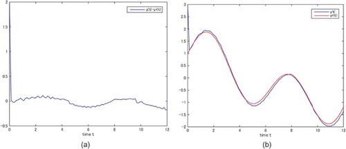
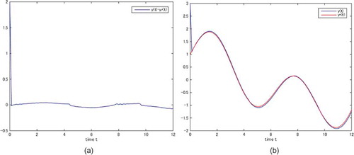
2. When the scaling gain $L$ is chosen as $L=300$, the tracking error obtained is about 0.075 as shown in Figure 2.

Figure 2. (a) Tracking error $y(t)-y_r(t)$ for L= 300. (b). The trajectories of $x_1(t)$,$y_r(t)$ for L= 300.

4. Conclusion

In this paper, we extend the result in (Alimhan et al., 2019) to solve the global practical tracking problem for a class of high-order nonlinear time-varying delays systems by state feedback. Under some mild-growth conditions, we first construct a state feedback controller with an adjustable scaling gain. Then, With the aid of a Lyapunov–Krasovskii functional, the scaling gain is adjusted to dominate the time-delay nonlinearities bounded by the growth conditions and make the tracking error arbitrarily small while all the states of the closed-loop system remain to be bounded.

Additional information

Funding

The work has been performed under grant projects of “Development of technologies for multilingual automatic speech recognition using deep neural networks” AP05131207 (2018–2020) at the Institute of Information and Computational Technologies CS MES Republic of Kazakhstan.

Notes on contributors

Keylan Alimhan

Keylan Alimhan received the M.S. degree in Information Sciences in 1998 from Tokyo Denki University (TDU), Japan and he finished his doctoral candidate course work in 2003 at TDU. In March 2009, he received the Doctor of Science degree in Mathematical Sciences from Graduate School of Science and Engineering of TDU. From 1985 to 1996, he served as an Assistant Professor in the Department of Mathematics, XU. From 2003 to 2004, he was a Research Associate in the Department of Information Sciences, TDU. From 2004 to present, he served as a Instructor, Assistant Professor and Research Fellow in School of Science and Engineering, TDU. Since September 2014, he has been with Faculty of Mechanics and Mathematics, Eurasian National University by named L.N.Gumilev as a Visiting Professor. His main research interests include nonlinear control theory, in particular, output feedback control of nonlinear systems and nonlinear robust control.

Appendix

To design state feedback controllers for the time-varying delay systems (1), we recall in this section the definition of homogeneous function and some useful lemmas to be used throughout this paper.

Definition A1 (Rosier, 1992). For a set of coordinates $x=\left(x_1,\dots ,x_n\right)\in R^n$ and an η-tuple $r=(r_1,\dots ,r_n)$ of positive real numbers we introduce the following definitions.

1. A dilation ${\mathrm{\Delta }}_s(x)$ is a mapping defined by ${\mathrm{\Delta }}_s^r(x)=\left(s^{r_1}{x}_1,\cdots ,s^{r_n}{x}_n\right),$ $\mathrm{\forall }x=(x_1,\dots ,x_n)\in R^n,$

   $\mathrm{\forall }s>0$, where $r_i$ are called the weights of the coordinate. For simplicity of notation, the dilation weight is denoted by $\mathrm{\Delta }=(r_1,\dots ,r_n)$.

2. A function $V\in C(R^n,R)$ is said to be homogeneous of degree $\tau$ if there is a real number $\tau \in R$

   such that $V({\mathrm{\Delta }}_s^r(x))=s^{\tau }V(x_1,\cdots ,x_n),\mathrm{\forall }x\in R^n-\left\{0\right\}$.

3. A vector field $f\in C(R^n,R^n)$ is said to be homogeneous of degree $\tau$ if the component $f_i$ is homogeneous of degree $\tau +r_i$ for each i, that is, $f_i({\mathrm{\Delta }}_s^r(x))=s^{\tau +r_i}{f}_i(x_1,\cdots ,x_n),$ $\mathrm{\forall }x\in R^n,$ $\mathrm{\forall }s>0,$ for $i=1,\dots ,n$.

4. A homogeneous$p$-norm is defined as ${∥x∥}_{\mathrm{\Delta },p}={\left({{\sum }_{i=1}^n\left|x_i\right|}^{p/r_i}\right)}^{1/p},\mathrm{\forall }x\in {\mathbb{R}}^n,p\ge 1$.

For the simplicity, write ${∥x∥}_{\mathrm{\Delta }}$ for ${∥x∥}_{\mathrm{\Delta },2}$.

Next, we introduce several technical lemmas which will play an important role and be frequently used in the later control design.

Lemma A1 (Rosier, 1992). Denote $\mathrm{\Delta }=(r_1,\dots ,r_n)$ as dilation weight, and suppose $V_1(x)$ and $V_2(x)$ are homogeneous functions with degree ${\tau }_1$ and ${\tau }_2$, respectively. Then, $V_1(x)V_2(x)$ is also homogeneous function with a degree of ${\tau }_1+{\tau }_2$ with respect to the same dilation Δ.

Lemma A2 (Rosier, 1992). Suppose $V:R^n\to R$ is a homogeneous function of degree $\tau$ with respect to the dilation weight $\mathrm{\Delta }$. Then, the following (i) and (ii) hold:

1. $\mathrm{\partial }V/\mathrm{\partial }{x}_i$ is also homogeneous of degree $\tau -r_i$ with $r_i$ being the homogeneous weight of $x_i$.

2. There is a constant $\sigma >0$ such that $V(x)\le \sigma {∥x∥}_{\mathrm{\Delta }}^{\tau }$. Moreover, if $V(x)$ is positive definite, there is a constant $\rho >0$ such that $\rho {∥x∥}_{\mathrm{\Delta }}^{\tau }\le V(x)$.

Lemma A3 (Polendo & Qian, 2006). For all $x,y\in R$ and a constant $p\ge 1$ the following inequalities hold:

1. ${\left|x+y\right|}^p\le 2^{p-1}\left|x^p+y^p\right|$, ${\left(\left|x\right|+\left|y\right|\right)}^{1/p}\le {\left|x\right|}^{1/p}+{\left|y\right|}^{1/p}$$\le 2^{\left(p-1\right)/p}{\left(\left|x\right|+\left|y\right|\right)}^{1/p}$

   If $p\in R_{odd}^{\ge 1}$, then

2. ${\left|x-y\right|}^p\le 2^{p-1}\left|x^p-y^p\right|$ and $\left|x^{1/p}-y^{1/p}\right|\le 2^{\left(p-1\right)/p}{\left|x-y\right|}^{1/p}.$

Lemma A4 (Polendo & Qian, 2007). Let $c,d$ be positive constants. Then, for any real-valued function $\gamma (x,y)>0$, the following inequality holds: .

${\left|x\right|}^c{\left|y\right|}^d\le \frac{c}{c+d}\gamma (x,y){\left|x\right|}^{c+d}+\frac{d}{c+d}{\gamma }^{-c/d}(x,y){\left|y\right|}^{c+d}.$

References

- Alimhan, K., & Inaba, H. (2008a). Practical output tracking by smooth output compensator for uncertain nonlinear systems with unstabilisable and undetectable linearization. International Journal of Modelling, Identification and Control, 5, 1–13. doi:10.1504/IJMIC.2008.021770
- Alimhan, K., & Inaba, H. (2008b). Robust practical output tracking by output compensator for a class of uncertain inherently nonlinear systems. International Journal of Modelling, Identification and Control, 4, 304–314. doi:10.1504/IJMIC.2008.021470
- Alimhan, K., & Otsuka, N. (2011). A note on practically output tracking control of nonlinear systems that may not be linearizable at the origin. Communications in Computer and Information Science, 256 CCIS, 17–25.
- Alimhan, K., Otsuka, N., Adamov, A. A., & Kalimoldayev, M. N. (2015). Global practical output tracking of inherently non-linear systems using continuously differentiable controllers. Mathematical Problems in Engineering, Article ID 932097, 10.
- Alimhan, K., Otsuka, N., Kalimoldayev, M. N., & Adamov, A. A. (2016). Further results on output tracking problem of uncertain nonlinear systems with high-order nonlinearities. International Journal of Control and Automation, 9, 409–422. doi:10.14257/ijca.2016.9.1.35
- Alimhan, K., Otsuka, N., Kalimoldayev, M. N., & Tasbolatuly, N. (2019). Output tracking by state feedback for high-order nonlinear systems with time-delay. Journal of Theoretical and Applied Information Technology, 97(3), 942–956.
- Chadli, M., & Borne, P. (2013). Multiple models approach in automation Takagi-Sugeno fuzzy systems. John Wiley & Sons. ISBN:9781848214125.
- Chadli, M., & Guerra, T. M. (2012). LMI solution for robust static output feedback control of discrete Takagi–Sugeno fuzzy models. IEEE Transactions on Fuzzy Systems, 20(6), 1160–1165. doi:10.1109/TFUZZ.2012.2196048
- Chadli, M., Maquin, D., & Ragot, J. (2002). Static output feedback for Takagi-Sugeno systems: An LMI approach. 10th Mediterranean Conference on Control and Automation.
- Chai, L. (2013). Global output control for a class of inherently higher-order nonlinear time-delay systems based on homogeneous domination approach. Discrete Dynamics in Nature and Society, Article ID 180717, 6.
- Gao, F., & Wu, Y. (2015). Further results on global state feedback stabilization of high-order nonlinear systems with time-varying delays. ISA Transactions, 55, 41–48. doi:10.1016/j.isatra.2014.08.014
- Gao, F., Wu, Y., & Yuan, F. (2016). Global output feedback stabilisation of high-order nonlinear systems with multiple time-varying delays. International Journal of Systems Science, 47(10), 2382–2392. doi:10.1080/00207721.2014.998318
- Gao, F., Yuan, F., & Wu, Y. (2013). Global stabilisation of high-order non-linear systems with time-varying delays. IET Control Theory & Applications, 7(13), 1737–1744. doi:10.1049/iet-cta.2013.0435
- Gong, Q., & Qian, C. (2005). Global practical output regulation of a class of non-linear systems by output feedback. Proceeding of the 44th IEEE Conference on Decision and Control, and the European Control Conference (pp. 7278–7283). Seville, Spain.
- Gong, Q., & Qian, C. (2007). Global practical output regulation of a class of nonlinear systems by output feedback. Automatica, 43(1), 184–189. doi:10.1016/j.automatica.2006.08.008
- Jia, X., & Xu, S. (2015). Global practical tracking by output feedback for nonlinear time-delay systems with uncertain polynomial growth rate. Proceeding of the 34th Chinese Control Conference (pp. 607–611).
- Jia, X., Xu, S., Chen, J., Li, Z., & Zou, Y. (2015). Global output feedback practical tracking for time-delay systems with uncertain polynomial growth rate. Journal of the Franklin Institute, 352, 5551–5568. doi:10.1016/j.jfranklin.2015.08.012
- Jia, X., Xu, S., & Ma, Q., Qi, Z., & Zou, Y. (2016). Global practical tracking by output feedback for a class of non-linear time-delay systems. IMA Journal of Mathematical Control and Information, 33, 1067–1080. doi:10.1093/imamci/dnv017
- Khalil, H. K. (1996). Nonlinear systems. Upper Saddle River, NJ: Prentice-Hall.
- Lin, W., & Pongvuthithum, R. (2003). Adaptive output tracking of inherently nonlinear systems with nonlinear parameterization. IEEE Transactions on Automatic Control, 48(10), 1737–1749. doi:10.1109/TAC.2003.817922
- Polendo, J., & Qian, C. (2006). A universal method for robust stabilization of nonlinear systems: Unification and extension of smooth and non-smooth approaches. Proceeding of the American Control Conference (pp. 4285–4290).
- Polendo, J., & Qian, C. (2007). A generalized homogeneous domination approach for global stabilization of inherently nonlinear systems via output feedback. International Journal of Robust and Nonlinear Control, 7(7), 605–629. doi:10.1002/rnc.1139
- Qian, C., & Lin, W. (2002). Practical output tracking of nonlinear systems with uncontrollable unstable linearization. IEEE Transactions on Automatic Control, 47, 21–36.
- Rosier, L. (1992). Homogeneous Lyapunov function for homogeneous continuous vector fields. Systems & Control Letters, 19, 467–473. doi:10.1016/0167-6911(92)90078-7
- Sun, Z., Xie, X., & Liu, Z. (2013). Global stabilization of high-order nonlinear systems with multiple time delays. International Journal of Control, 86, 768–778. doi:10.1080/00207179.2012.760046
- Sun, Z., Liu, Y., & Xie, X. (2011). Global stabilization for a class of high-order time-delay nonlinear systems. International Journal of Innovative Computing, Information and Control, 7, 7119–7130.
- Sun, Z. Y., & Liu, Y. G. (2008). Adaptive practical output tracking control for high-order nonlinear uncertain systems. Acta Automatica Sinica, 34, 984–989. doi:10.1016/S1874-1029(08)60048-8
- Yan, X., & Song, X. (2014). Global practical tracking by output feedback for nonlinear systems with unknown growth rate and time delay. The Scientific World Journal, Article ID 713081, 7.
- Zhai, J., & Fei, S. (2011). Global practical tracking control for a class of uncertain non-linear systems. IET Control Theory and Applications, 5, 1343–1351. doi:10.1049/iet-cta.2010.0294
- Zhang, N., Zhang, E., & Gao, F. (2014). Global stabilization of high-order time-delay nonlinear systems under a weaker condition. Abstract and Applied Analysis, Article ID 931520, 8.
- Zhang, X., Lin, W., & Lin, Y. (2017). Nonsmooth feedback control of time-delay nonlinear systems: A dynamic gain based approach. IEEE Transactions on Automatic Control, 62, 438–444. doi:10.1109/TAC.2016.2562059