One method of generating synthetic data to assess the upper limit of machine learning algorithms performance

Abstract

Based on statistics from the World Nuclear Association, Kazakhstan has the highest uranium production in the world. Most of the uranium in the country is mined via in-situ leaching and the accurate classification of lithologic composition using electric logging data is economically crucial for this type of mining. In general, this classification is done manually, which is both inefficient and erroneous. Information technology tools, such as predictive analytics with Supervised Machine Learning (SML) algorithms and Artificial Neural Networks (ANN) models, are nowadays widely used to automate geophysical processes, but little is known about their application for uranium mines. Previous experiments showed an ANN accuracy of about 60% in the task of lithological interpretation of logging data. To determine the upper limit of the accuracy of machine learning algorithms in such task and for indirect assessment of the experts’ influence, a digital borehole model was developed. This made it possible to generate a complete set of data avoiding subjective expert assessments. Using these data, the work of various ML algorithms, both simple (kNN) and deep learning models (LSTM), was evaluated.

KEYWORDS:

• Machine learning (ML)
• Supervised machine learning (SML)
• simulated borehole
• accuracy
• precision
• recall
• artificial neural network (ANN)
• SVM
• XGBOOST
• LSTM

PUBLIC INTEREST STATEMENT

Kazakhstan accounts for 40% of the world’s uranium mining, which is extracted by the method of in-situ leaching. Moreover, the correct interpretation of geophysical data plays an important role in the process of uranium production. This process is quite complex and time consuming. For a correct interpretation, as a rule, a lot of experience is required in a particular field. To increase the efficiency and accuracy, it is proposed to use machine learning algorithms that, using the experience of experts, could perform lithological classification automatically. In this work, we propose a method for generating “ideal” geophysical data for assessing the upper limit of the quality of classifiers and provide comparative results for evaluating classifiers of various types (artificial neural network, gradient boosting, support vector machines, Long short-term memory) on real data. The use of machine learning systems for the interpretation of geophysical data will improve the economic efficiency and environmental friendliness of uranium mining in Kazakhstan.

1. Introduction

Since 2009, Kazakhstan is the world leader in uranium mine production generating over one-third of the total uranium global volume. The uranium production has grown 3.5 times in the last 7 years in Kazakhstan, demonstrating a strong and compelling need in applying novel ideas and technologies for uranium mining. Optimization of uranium commercial production processes from mining ores to nuclear power is a cornerstone requirement for KazAtomProm, for example, which is an effective and sustainable Nationwide organization.

Automation of production processes, e.g. Geophysical Data Interpretation for Boreholes (GDIB) in uranium mines, is just one of many ways this optimization can be achieved. Erroneous and inaccurate results from geophysical data analysis may lead to serious financial losses on different levels: from overall decrease of active boreholes to unjustified labor cost and low volume production. GDIB processes can specifically be used for analyzing lithological composition of the borehole, while predictive analytics with SML algorithms and ANN models for automation and streamlining the overall analytical process.

The success of data interpretation processes depends on properly prepared input data. Quality, content, and format of the input data directly affect the machine learning processes, and subsequently the final accuracy of classification. The accuracy of automated log data classification to a great extent depends on expert’s manual assessment because it is used as input for training ML automatic classifiers. However, cross-comparison of assessments for core sampling provided by different experts shows significant discrepancies. Specifically, the difference between assessments grows higher with decreased value of geological samples (e.g. sandstones have more deviations in manual classification than claystones). Here, we aim to capture the nature of this phenomenon and to define the limits of automatic classification while applying ANN that are trained on expert assessment input data.

The following parts constitute our efforts and presented in this paper:

Part 1. Literature review, with delineation of known issues for ANN classification of log data from uranium mines;

Part 2. Synthetic Log Data;

Part 3. Algorithm of generating synthetic Log data;

Part 4. Brief description of used ML methods;

Part 5. Results with real and synthetic data;

Part 6. Conclusion, with summary of results and recommendations for the next set of analytical experiments design.

2. Literature review

Since 1970, the artificial neural network (ANN) modeling is widely used in petrography to analyze lithologic log data, to evaluate geo-mineral resources, for deep seismic sounding, and for many other geophysical analyses (Aleshin & Lyakhov, 2001; Baldwin, Bateman, & Wheatley, 1990; Benaouda, Wadge, Whitmark, Rothwell, & MacLeod, 1999; Borsaru, Zhou, Aizawa, Karashima, & Hashimoto, 2006; Kapur, Lake, Sepehrnoori, Herrick, & Kalkomey, 1998; Rogers, Chen, Kopaska-Merkel, & Fang, 1995; Rogers, Fang, Karr, & Stanley, 1992; Saggaf & Nebrija, 2003; Tenenev, Yakimovich, Senilov, & Paklin, 2002; Van der Baan & Jutten, 2000; Yelbig & Treitel, 2001). (Kostikov, 2007) thoroughly describes methods for boreholes geophysical data interpretation based on the transformation of log diagrams using multi-layer neural network. Several publications demonstrate the application of feedforward neural network for interpretation of geophysical data from uranium deposits (Amirgaliev, Iskakov, Kuchin, & Muhamediev, 2013a, 2013b; Muhamediyev, Amirgaliev, Iskakov, Kuchin, & Muhamedyeva, 2014a).

In Kazakhstan uranium is mined via sub-surface in-situ leaching of boreholes, which is one of the low-cost and ecologically safe mining methods (Yashin, 2008). Moreover, the cost-efficiency of uranium ore mining depends on the speed and accuracy of geophysical data and its interpretation. Most of the collected data generated via electricity-based methodology such as logging of apparent resistance (АR), spontaneous polarization potential (SP), and induction log (IL). Log results are usually presented as diagrams, which in turn used by experts to manually assess the depth and value of the uranium deposits. In the course of data interpretation, an expert usually extracts information about bedding rock layers and performs lithological classification describing borehole throughout its depth. This manual process of borehole core sampling data processing has inevitably slow rate of data generation and low accuracy. From uranium production point of view, the importance of electrical log data accuracy from uranium boreholes is hard to underestimate. Ultimately, these data define the location for a long-term installation of an expensive filter that is required for uranium sub-surface mining via in-situ leaching.

Here, we used historically generated classifications from two minefields (~200 boreholes) to train our ANN model with ML algorithms.

In general ANN models are capable of resolving poorly formalized tasks (Neurocomputers, 2004) however in our case, this approach is predisposed to several challenges:

1. Inconsistency of experts’ opinion in data assessment;

2. Requirement for equal and large number of examples from each class of data;

3. ANN inability to interpret resulting outcome;

4. Requirement for thorough preparation of input data prior to analysis (e.g. outliers’ removal, normalization, data smoothing).

There is a number of publications focused on tasks and issues related to automatic interpretation of log data from uranium deposits. For example, results of analytical testing with ANN as an approach for log data classification can be found in publications (Kuchin et al., 2011; Muhamedyev, Kuchin, & Muhamedyeva, 2012; xxxx, 2011), while several ML methods and their comparative results described in publications (Amirgaliev et al., 2014; Muhamedyev et al., 2015). There, it was shown that feedforward neural network demonstrates a much better classification’s quality when compared to k-nearest neighbor (k-NN) or support vector machine (SVM) algorithms. Furthermore, results from a combination of ML algorithms applied to a similar underlying task were reviewed in publications (Muhamediyev, Amirgaliev, Iskakov, Kuchin, & Muhamedyeva, 2014b; Muhamedyev, Iskakov, Gricenko, Yakunin, & Kuchin, 2014). This article raises the question of the upper limit of the quality of classification for various MO algorithms in relation to this problem.

3. Synthetic log data

Due to inherent issues with log data classification (e.g. limited information about actual distribution of lithotypes along the borehole axes), the accurate assessment of classification’s quality for real geophysical data is not feasible. Core sampling is usually done for just a few boreholes with limited interpretation throughout the well’s depth. That is why the system of ML classification relies on expert’s assessment data. In other words, the system of ML classification is trained primarily on expert’s opinion/assessment, assuming that it is accurate. This approach, however, leads to a value paradox where actual merit of such expert’s interpretation has many inherent contradictions.

As was mentioned above, our earlier experiments demonstrated that automatic classification with feedforward neural network generally performs with ~60% accuracy.

The question arises, is a good result or not, what the upper limit of the accuracy of ML algorithms in such a task to which you want to strive for. The answer will also allow indirectly assess the impact of the inconsistency of expert assessments.

To test the quality of ML system performance, one can generate synthetic dataset equivalent to real log data by one or several parameters. These synthetic data would fit basic physical criteria for log instruments and have properties of the ore from uranium deposits. Of course, such evaluation is not exhaustively complete, yet it can demonstrate algorithm’s potentials and limitations, as well as to indirectly provide us with insight on expert assessment’s value. Additionally, the extend of contradictions in expert’s assessment can be elucidated simply by comparing the results of assessment performed by several independent experts.

The only true and reliable definition of lithologic composition along the borehole axe comes from the actual coring (collection of ore samples from the well). However, even that does not assure complete information collection because the lithotype extraction from sedimentary layers (characteristic to uranium deposits in Kazakhstan), in general, does not exceed 80%. Moreover, additional errors are introduced during mapping the core sampling to the borehole depth and during core data description itself. It is challenging to identify and account for all these errors. When reliable information about lithologic composition of the borehole core section is lacking, and both electrical log data and coring provide just approximate values, the outcome from modeling of registered log signal for predefined distribution of lithotype along the borehole core with known physical properties seems not just practical, but best quality. Thus, this approach allows for the generation of artificial but fully defined log values, unmistakably linked to a specific kind of lithotypes.

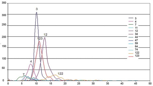
Physical properties of each type of lithotype (e.g. apparent resistance, AR) have specific range of values. Distribution of values within that range can be explored during geological expedition or in the laboratory. During geological expedition the coring is done, the laboratory analysis is performed, and physical property of each type of ore, including their characteristic AR values, is being registered (Methodical recommendations, 2003; Technical instruction, 2010). Examples of typical AR-values distribution are shown in Figure 1 (the diagram is a courtesy of GeoTechnoService organization). On the graph, the apparent resistance (ohm·m) is plotted along the X-axis, and the number of intervals having such resistance is plotted along the Y-axis. For example, for lithotype 3, the peak value indicates that at 310 intervals where this lithotype is present, the apparent resistance value is about 10 ohm·m. At the same time, number of intervals with AR value of more than 15 and less than 7 ohm·m is negligible. Explanation of lithotype codes is given in Appendix 1.

(https://drive.google.com/open?id=1jJugEzOckV4fM95bD4xg21AfK44NtlQt)

As you can see, there is a significant overlap between AR distributions for 13 lithotypes in GeoTechnoService study. The diagrams also suggest that a normal distribution curve within a given value range can be used for modeling in the first order of approximation. On the other hand, the values for spontaneous polarization potential (SP) are more complicated for simulation, because they depend on at least two external factors: properties of drilling solution and groundwater mineralization.

Figure 1. Distribution of AR values for 13 lithotypes

(Each lithotype is color/number coded).

Once the power distribution curve for lithotype layer is defined, the AR values are chosen for each 10cm-increment of sub-layer within that geological layer, which in turn allows to build an AR distribution curve throughout borehole’s core.

To accurately model the registered AR curve, it is also important to take into account the parameters of drilling instrument (probe type, distance between electrodes), borehole’s diameter, and properties of drilling solution among other factors. Thus, we develop an artificial AR log record, which would correspond to a given lithotype composition, and the validity of information about it will be 100% accurate. Same approach is used for modeling the SP distribution curve.

Synthetic AR and SP data can further be used for tuning and improving various ML algorithms. The best approximation of the model to actual conditions allows for increased accuracy of real data recognition and for outlining the upper limit of detection accuracy.

Process of synthetic data generation consists of three parts:

1. Lithological types generation

2. Physical properties values generation

3. Measuring process simulation

First, a sequence of lithologic layers is generated based on statistical distribution of lithotype occurrence (e.g. 20% of layers are clay, 50% are sand layers, etc.) and typical layer power for modeled horizon of the given minefield (e.g. 1–4 m for sand layer, 0.2–2 m of clay, 0.2–0.5 m of sandstones, etc.).

There is also an option to set a static layer distribution, for example, to copy lithological layers of an existing borehole. This option was used further in the section to validate the generation algorithm.

Then, for each 10-cm increment of sub-layer inside each of the generated layers, an AR value is generated using statistical distribution from existing data. In current implementation, a Gaussian distribution is used, since AR and SP values distribution is close to Gaussian, as illustrated by Figure 1.

The last step is measuring process simulation. Physical properties of drilling solution and groundwater, borehole diameter, and drilling instrument parameters may affect log-registered values for AR and SP. In our model, we used parameters of drilling instrument as main factors affecting registered values.

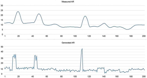
The logging data is measured with 10-cm increment; however, typical distance between electrodes is 1 m, which means that for measured value of each of the 10 cm interval is affected by physical properties of the surrounding soil. The extent to which the measured value is affected by surrounding soil is set by numerical coefficients, which are one of the parameters of the synthetic data generation process along with lithotypes and physical properties statistical distributions. Results for AR-values generation by the drilling instrument model are shown in Figure 2 (bottom plot shows generated AR values, while the top plot is the result of measurement simulation). The figure illustrates two main factors, which make classification based on measured physical values inherently difficult:

1. The measured data is very smooth, averaged, which means that the actual bounds of each layer are difficult to distinguish.

2. When measuring small layers with high AR value, the power of the layer can be not enough to saturate the measuring instrument, which leads to much lower AR value being measured. This problem can be partially solved by taking the curvature of the signal into account.

Figure 2. “Measured” and generated AR values

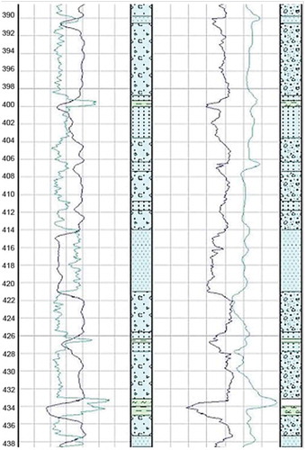
To validate models’ competence, we used some boreholes from our training set to model “measured” AR and SP values for a given distribution of lithotypes along borehole’s core. Results for one of the boreholes (Figure 3) show a nice alignment between modeled and actual log-data. The fact that the modeled AR diagram is smoother compared to actual data can be explained by the incomplete input of factors such as borehole diameter, errors of measurement, and other. The modeled SP diagram is more expressive than the actual one; however, it is practically impossible to find a good quality actual SP record as it requires special preparation (e.g. solution, measurement conditions) that is hard to fulfill.

Figure 3. Modeled (left column) and actual (right column) log-data for AR (blue) and SP (green) values

4. Brief description of used Ml methods

Machine learning methods are divided into two broad groups. (Hamza Awad Hamza et al., 2012; Muhamedyev, 2015; Oladipupo Ayodele, 2010):

- Unsupervised Learning (UL) (Hastie, Tibshirani, & Friedman, 2009).

- Supervised Learning (SL)(Kotsiantis, Zaharakis, & Pintelas, 2007).

UL methods solve the problem of clustering, when the set of not previously marked objects is divided into groups by an automatic procedure, based on the properties of these objects. (Barbakh, Ying, & Fyfe, 2009; Jain, Murty, & Flynn, 1999).

SL methods solve the problem of classification or regression. The task of classification arises when in a potentially infinite set of objects there are finite groups of objects in some way indicated. Usually, the formation of groups is performed by an expert. The classification algorithm should, using this initial classification as a model, assign the following unmarked objects to a particular group, based on the properties of these objects.

In our case, since we have data marked up by experts, it is advisable to apply a group of SL methods which include k-Nearest-Neighbor (k-NN) (Altman, 1992), Logistic regression, Decision Tree (DT), Support Vector Classifier (Cortes & Vapnik, 1995) and a large family of artificial neural networks (ANN) (The Neural Network Zoo Posted, 2019; Zhang, 2000) and compositions of algorithms, for example, using boosting.

We shall briefly describe the listed algorithms and how to call them in programs. Note that the description of the logistic regression is for reference only. The logistic regression model is useful for understanding the SVM and ANN algorithms. Among the many ANNs, we have chosen to apply the “classic” feedforward neural networks in the form of a multilayer perceptron (MLP) and one of the varieties of deep learning networks (LSTM), which is successfully used to analyze time series.

4.1. Logistic regression

The algorithm is used when it is necessary to divide objects of two classes, for example, into “negative” and “positive”. In this case, the hypothesis function is required to fulfill the condition

$0\le h_{\theta }(x)\le 1$, what is achieved using a sigmoidal (logistic) function

(1) $h_{\theta }(x)=\frac{1}{1+e^{-{\theta }^{T}x}},$(1)

where $\mathrm{\Theta }$ parameter vector, x is a vector of input variables.

Selection of parameters $\mathrm{\Theta }$ after selecting the hypothesis function is performed to minimize the cost function of the form

(2) $J(\theta )=\left[-\frac{1}{m}\sum _{i=1}^m{y}^{(i)}log(h_{\theta }(x^{(i)}))+(1-y^{(i)})log(1-h_{\theta }(x^{(i)}))\right]+\frac{\lambda }{2m}\sum _{j=1}^n{\theta }_j^2,$(2)

where m is the number of training examples, $y^{(i)}$ is the class of the i-th object, $\lambda$ is the regularization parameter that allows you to control the degree of generalization of the algorithm.

For large $\lambda$, the algorithm will form more smoothed boundaries between classes.

Minimization of the cost function is achieved using the gradient descent algorithm, but also use the Conjugate gradient (Møller, 1993), BFGS, L-BFGS (Liu & Nocedal, 1989) (below lbfgs)

Although the logistic regression algorithm was originally proposed for classifying into two classes or One-vs-all, however, the current version of this model allows classification of objects of several classes when the multi_class parameter is set. The main adjustable parameter C is the inverse regularization quantity. The smaller it is, the stronger the regularization, that is, the more smooth the line separates the classes. The algorithm is called from the library sklearn.linear_model

from sklearn.linear_model import LogisticRegression

A classifier is created using the following command

clf = LogisticRegression(C = 1, solver = “lbfgs”)

4.2. kNN

The algorithm (Dudani, 1976; K-nearest neighbor algorithm, 2012) is based on counting the number of objects of each class in a sphere (hypersphere) with a center in an object being classified. The classified object belongs to the class whose objects are most in this area. If the weights of objects are not the same, then instead of counting the number of objects, we can sum up their weights. Thus, if in a sphere around an object being classified there are 10 standard objects of class A weighing 2 and 15 erroneous/border objects of class B with weights 1, then the classified object will be classified as class A.

The weights of objects in a sphere can be represented as inversely proportional to the distance to a recognizable object. Thus, the closer the object, the more significant it is for a given recognizable object. Depending on the modification of the algorithm, distances can be estimated using different metrics (DistanceMetric.html, 2019).

As a result, the classifier can be described as:

(3) $a(u;X^l)=arg\underset{y\in Y}{max}\sum _{i=1}^l[y_u^{(i)}=y]w(i,u),$(3)

where w (i, u) is the weight of the i-th neighbor of the recognized object u; (u; X^l) is the class of the object u, recognized by the sample X^l.

In general, it is one of the fastest, but inaccurate classification algorithms. Loading the corresponding library and creating the classifier is performed by commands.

from sklearn import neighbors

clf = neighbors.KNeighborsClassifier(n_neighbors = 311, p = 3)

The specified parameters (n_neighbors = 311, p = 3) were found by the GridSearchCV utility.

4.3. SVM

In the general case, support vectors are constructed in such a way as to minimize the cost function of the form:

(4) $J(\mathrm{\Theta })=C\sum _{i=1}^m{y}^{(i)}{S}_1({\mathrm{\Theta }}^T{f_k}^{(i)}(x^{(i)}))+(1-y^{(i)})S_0({\mathrm{\Theta }}^T{f_k}^{(i)}(x^{(i)}))+\frac{1}{2}\sum _{j=1}^m{\theta }_j^2$(4)

where $S_1$ and $S_0$ functions replace $log(h_{\theta })$ and $1og(1-h_{\theta })$ in the expression for logistic regression (2). Usually $S_1$ and $S_0$ are piecewise linear functions.

$f_k$ is a kernel function that determines the significance of the objects of the training set in the feature space. Often, a Gaussian function ${f_k}^{(i)}(x^{(i)})=exp\left(\frac{|x-x^{(i)}{|}^2}{2{\delta }^2}\right)$ is used, which for any x allows us to estimate its proximity to and thus form the boundaries between classes closer or more distant from the reference object, setting the value of $\delta$.

С- is a regularization parameter ($C=1/\lambda$).

Example of using a classifier:

from sklearn.svm import SVC

SVMclassifier = svm.SVC(kernel = “rbf”,C = 50,000,gamma = 0.0001)

The specified classifier parameters were found by the GridSearchCV utility.

4.4. XGBoost

The XGBoost algorithm (Extreme Gradient Boosting) is based on the concept of gradient boost introduced in Riedman, (2001) and provides optimized distributed gradient boost on decision trees (About XGBoost, 2019). The essence of boosting is that after calculating the optimal values of the regression coefficients and obtaining the hypothesis function $h_{\theta }(x)$ using some algorithm (a), an error is calculated and a new function $h_{b\theta }(x)$ is selected, possibly using another algorithm (b), so that it minimizes the previous error

$h_{\theta }(x^{(i)})+h_{b\theta }(x^{(i)})-y^{(i)}\to min$

In other words, it is a matter of minimizing the function:

(5) $J_b=\sum _{i=1}^{m}L(y^{(i)},h_{\theta }(x^{(i)})+h_{b\theta }(x^{(i)}))$(5)

where L is the error function, taking into account the results of the algorithms a and b. If $J_b(\theta )$ is still large, the third algorithm is selected (c), etc. Often decision trees of relatively shallow depth are used as algorithms (a), (b), (c), etc. To find the minimum of the $J_b(\theta )$ function, the value of the error function gradient is used.

$L(y^{(i)},h_{\theta }(x^{(i)}){)}_{i=1}^m$

Considering that the minimization of the function $J_b(h_{b\theta }(x^{(i)}){)}_{i=1}^m$ is achieved in the direction of the anti-gradient of the error function, the algorithm (b) is adjusted so that the target values are not $(y^{(i)}{)}_{i=1}^m$ but the antigradient ($-L^{\prime }(y^{(i)},h_{\theta }(x^{(i)}){)}_{i=1}^m$), that is, when training the algorithm (b) instead of $(x^{(i)},y^{(i)})$ pairs, $(x^{(i)},-L^{\prime }(y^{(i)},h_{\theta }(x^{(i)}))$ pairs are used.

Library loading and classifier creation are performed by commands:

import xgboost

clf = xgboost.XGBClassifier(nthread = 1)

4.5. MLP

Multilayer artificial neural networks (multilayer perceptron) are one of the most popular classifiers especially for the case of several classes. To adjust the weights $\theta$ of the neural network (network training), a cost function resembling the logistic regression cost function is used.

(6) $J(\mathrm{\Theta })=-\frac{1}{m}[\sum _{i=1}^m\sum _{k=1}^K\hspace{0.17em}{y_k}^{(i)}log(h_{\mathrm{\Theta }}(x^{(i)}){)}_k+(1-{y_k}^{(i)})log(1-h_{\mathrm{\Theta }}(x^{(i)}){)}_k]+\frac{\lambda }{2m}\sum _{l=1}^{L-1}\sum _{i=1}^{S_l}\sum _{j=1}^{S_{l+1}}({\mathrm{\Theta }}_{ji}^l{)}^2,$(6)

where L is the number of layers of the neural network; $s_l$ the number of neurons in the l layer; K is the number of classes (equal to the number of neurons in the output layer); $\mathrm{\Theta }$ weights matrix.

To minimize the error function (training) of a multi-layer ANN, an error back propagation algorithm (Back Propagation Error BPE) (Werbos, 1974) and its modifications aimed at accelerating the learning process are used. Loading the classifier and creating the corresponding object is as follows:

from sklearn.neural_network import MLPClassifier

clf = MLPClassifier(hidden_layer_sizes = (Aleshin & Lyakhov, 2001, 2001), alpha = 5, random_state = 0, solver = “lbfgs”).

4.6. LSTM

Long short-term memory (LSTM) is a kind of recurrent neural networks that can memorize values for short or long periods of training.

When an error is back propagating across large networks, the error transmitted from the output to the input will gradually decrease until it becomes disappearing small. To reduce this effect, the concept of a constant error carousel (CEC) was introduced in (Hochreiter & Schmidhuber, 1997). The CEC property is achieved by using a linear unit with a fixed internal link (s), which is the central element of the LSTM, around which the entire so-called memory cell is built. The j-th LSTM cell is denoted$c_j$. In addition to the “normal” input signal, it receives a signal from a multiplicative output element (output gate out gate) and a multiplicative input element (input gate in gate) with sigmoidal activation functions (in later literature is called forget gate). Inside the cell, there is an input and hidden layer with sigmoidal activation functions and a linear link that process the listed set of signals.

Out gate values:

(7) $y^{ou{t}_j}(t)=f_{ou{t}_j}(ne{t}_{ou{t}_j}(t)),$(7)

In gate values:

(8) $y^{i{n}_j}(t)=f_{i{n}_j}(ne{t}_{i{n}_j}(t)),$(8)

Where:

(9) $ne{t}_{ou{t}_j}(t)=\sum _u{w}_{ou{t}_{ju}}{y}^u(t-1),$(9)

(10) $ne{t}_{i{n}_j}(t)=\sum _u{w}_{i{n}_{ju}}{y}^u(t-1),$(10)

Network output:

(11) $In=ne{t}_{cj}(t)=\sum _u{w}_{c_{ju}}{y}^u(t-1),$(11)

The processing process includes five main stages indicated in numbers in Figure 4.

1) $g(ne{t}_{cj}(t))$

2) $g(ne{t}_{cj}(t))y^{i{n}_j}(t)$

3) $s(0)=0,s_{cj}(t)=s_{cj}(t-1)+y^{i{n}_j}(t)g(ne{t}_{cj}(t))$

4) $h(s_{cj}(t))$

5) Out =$y^{c_j}(t)=y^{ou{t}_j}(t)h(s_{cj}(t))$

Figure 4. LSTM memory cell (Hochreiter & Schmidhuber, 1997)

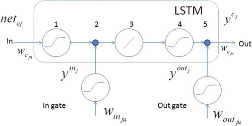
Such an architecture allows to “forget” that part of the information that is no longer needed in the new t + 1 step, while adjusting the weights of the input gate, and add a new piece of information, adjusting the weights of the output gate.

The LSTM network is constructed from a sequence of described cells so that the input signal is fed to the network inputs and input gates of all memory cells, and the output cells are fed to the inputs and input gates of the following memory cells (Figure 5) (Keras LSTM tutorial, 2019).

Figure 5. LSTM network architecture implemented in Keras

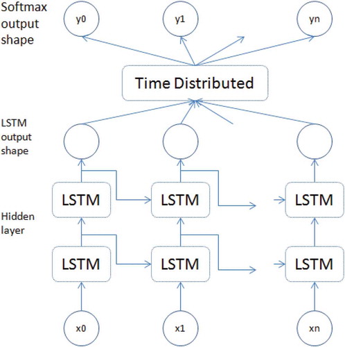
LSTM is effective in working with time series. The task of lithological classification can be considered as the task of working with a series of values, but not in time but in space (in depth).

Classifier loading and creating the corresponding object is as follows:

keras.layers.recurrent import LSTM

model = Sequential()

model.add(Bidirectional(LSTM(50, input_shape = (10, 2))))

5. Results with real and synthetic data

After linear normalization, the real and simulated data were fed to the input of several classifiers (ANN, kNN, SVM, XGBOOST, LSTM) in the form of a “floating window” (Figure 6).

The use of “floating data windows” is a common method of analyzing data sequences, for example, time series or, as in our case, the dependence of recorded physical parameters on the depth. Since the expert takes into account the form of the logging curve when evaluating the data, it is reasonable to submit to the input data in a form of floating window with the size of n + 1 + n points. That is, n measurements above, the current value and n measurements below the current value are considered. The next window is formed in a similar way, shifting one point below.

Figure 6. Floating data window

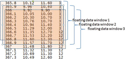
Since the logging probe length is 1 m, which corresponds to 10 depth measurements, it is natural to set n = 5. Presenting data in the form of a floating window allows, to some extent, to take into account the form of the curve, and not just the value of recorded parameter at a specific depth.

For each of the 36 boreholes from the dataset, its “ideal” variant was simulated. The boreholes were divided into training and test sets in the ratio of 30/6. It should be noted that for the correct division into training and test sets in this case it was impossible to use sklearn.model_selection.train_test_split or similar functions due to the presence of a floating window. Due to the fact that the classes are not balanced, the weighted F1 was chosen as the main metric of quality (algorithm performance). For example, one of the possible combinations (lithotype code: number of values): 6: 4504, 4: 8177, 3: 21,746, 1: 15,653, 5: 251, 7: 4494, 9: 5. For this reason, weighted precision (Prec), weighted recall (Recall) and weighted F1 are given in tables to assess algorithms performance.

Several models of classifiers ANN, LSTM, and XGBoost have been tested (Described in Appendix 2 https://drive.google.com/open?id=1eJk8XIeOfYoBCjvlKjbuBCAjWyDEHU8n). For each type of classifier, a model that showed on average the best result for all folds was selected. Since the classification result for ANN and LSTM depends on the initial initialization, in order to increase statistical reliability, training, and evaluation of the results were carried out five times. That is, each model of these two types of classifiers was re-initiated, trained, and evaluated. The full results of computational experiments are given in Appendix 3(https://drive.google.com/open?id=1al9QqJGydtAwNzapWribV3rBPzkSPdvC). The tables below show the results for different partitions. It can be seen that the accuracy of the classification significantly depends on the splitting, in addition, even on the ideal data; the accuracy of the classifiers differs significantly. The results of the classification are shown in Table 1.

Table 1. Results of classifiers on simulated data

Test boreholes	ANN				SVM				LSTM
	Acc	Prec	Recall	F1	Acc	Prec	Recall	F1	Acc	Prec	Recall	F1
0-5	0,856	0,869	0,856	0,857	0,842	0,857	0,842	0,846	0,855	0,872	0,855	0,857
6-11	0,859	0,864	0,859	0,854	0,831	0,826	0,831	0,829	0,879	0,878	0,879	0,875
12-17	0,819	0,835	0,819	0,820	0,804	0,818	0,804	0,805	0,853	0,863	0,853	0,855
18-23	0,923	0,924	0,923	0,922	0,905	0,904	0,905	0,904	0,940	0,939	0,940	0,938
24-29	0,912	0,912	0,912	0,911	0,891	0,891	0,891	0,888	0,950	0,950	0,950	0,950
30-35	0,897	0,902	0,897	0,896	0,892	0,891	0,892	0,891	0,951	0,952	0,951	0,951
MEAN	0,878	0,884	0,878	0,877	0,861	0,866	0,861	0,861	0,905	0,909	0,905	0,904
DISP	0,0016	0,0012	0,0016	0,0015	0,0017	0,0012	0,0017	0,0016	0,0022	0,0018	0,0022	0,0022

Table

Test boreholes	XGBOOST				KNN
	Acc	Prec	Recall	F1	Acc	Prec	Recall	F1
0-5	0,852	0,869	0,852	0,855	0,441	0,372	0,441	0,373
6-11	0,885	0,887	0,885	0,880	0,468	0,496	0,468	0,409
12-17	0,850	0,862	0,850	0,852	0,475	0,469	0,475	0,400
18-23	0,950	0,950	0,950	0,950	0,521	0,547	0,521	0,453
24-29	0,954	0,954	0,954	0,954	0,417	0,501	0,417	0,353
30-35	0,949	0,950	0,949	0,948	0,471	0,417	0,471	0,398
MEAN	0,907	0,912	0,907	0,907	0,466	0,467	0,466	0,398
DISP	0,0025	0,0019	0,0025	0,0024	0,0012	0,0040	0,0012	0,0012

The same classifiers have been applied to real data.

On real data, the accuracy of all classifiers is significantly lower, it is also clear that ANN, LSTM, XGBOOST show the best results. From Table 2 it can be seen that the splitting at which wells 24–29 fall into the test set leads to the worst results. In this regard, the idea arose to try to replace them with “ideal” generated data. Since the results depend on dataset splitting, for subsequent experiments we fixed splitting (0–6 test boreholes). The results are shown in Table 3 (ORIGINAL – source data, DATA_ID = True – mark synthetic data, DATA_ID = False – not mark synthetic data).

Table 2. Results of classifiers on real data

Test boreholes	ANN				SVM				LSTM
	Acc	Prec	Recall	F1	Acc	Prec	Recall	F1	Acc	Prec	Recall	F1
0-5	0,573	0,521	0,573	0,519	0,576	0,538	0,576	0,515	0,463	0,436	0,463	0,442
6-11	0,507	0,542	0,507	0,439	0,497	0,538	0,497	0,420	0,398	0,477	0,398	0,409
12-17	0,531	0,470	0,531	0,462	0,550	0,448	0,550	0,462	0,460	0,441	0,460	0,434
18-23	0,553	0,534	0,553	0,515	0,529	0,460	0,529	0,465	0,463	0,474	0,463	0,463
24-29	0,371	0,326	0,371	0,312	0,379	0,301	0,379	0,323	0,399	0,381	0,399	0,367
30-35	0,479	0,443	0,479	0,445	0,458	0,427	0,458	0,415	0,479	0,496	0,479	0,462
MEAN	0,502	0,473	0,502	0,449	0,498	0,452	0,498	0,433	0,444	0,451	0,444	0,430
DISP	0,0052	0,0067	0,0052	0,0056	0,0051	0,0077	0,0051	0,0042	0,0013	0,0017	0,0013	0,0014

Table

Test boreholes	XGBOOST				KNN
	Acc	Prec	Recall	F1	Acc	Prec	Recall	F1
0-5	0,547	0,523	0,547	0,506	0,388	0,315	0,388	0,321
6-11	0,528	0,554	0,528	0,491	0,444	0,473	0,444	0,364
12-17	0,525	0,481	0,525	0,453	0,432	0,368	0,432	0,348
18-23	0,550	0,536	0,550	0,515	0,452	0,448	0,452	0,383
24-29	0,395	0,372	0,395	0,343	0,365	0,365	0,365	0,292
30-35	0,507	0,509	0,507	0,495	0,401	0,415	0,401	0,335
MEAN	0,509	0,496	0,509	0,467	0,414	0,397	0,414	0,341
DISP	0,0033	0,0042	0,0033	0,0042	0,0012	0,0035	0,0012	0,0010

Table 3. Classification results for partial replacement of real data with simulated data

DATA ID	ANN				SVM				XGBOOST				KNN
	Acc	Prec	Recall	F1	Acc	Prec	Recall	F1	Acc	Prec	Recall	F1	Acc	Prec	Recall	F1
FALSE	0,525	0,500	0,525	0,493	0,567	0,518	0,567	0,509	0,515	0,497	0,515	0,494	0,382	0,314	0,382	0,304
MEAN	0,525	0,500	0,525	0,493	0,567	0,518	0,567	0,509	0,515	0,497	0,515	0,494	0,382	0,314	0,382	0,304
DISP	0,0002	0,0018	0,0002	0,0010	—–	—–	——	—–	—–	—–	—–	—–	—–	—–	—–	—–
TRUE	0,568	0,536	0,568	0,514	0,585	0,529	0,585	0,530	0,547	0,509	0,547	0,501	0,392	0,304	0,392	0,315
MEAN	0,568	0,536	0,568	0,514	0,585	0,529	0,585	0,530	0,547	0,509	0,547	0,501	0,392	0,304	0,392	0,315
DISP	0,0001	0,0002	0,0001	0,0001	—–	—–	——	—–	—–	—–	—–	—–	—–	—–	—–	—–
ORIGINAL	0,573	0,521	0,573	0,519	0,576	0,538	0,576	0,515	0,547	0,523	0,547	0,506	0,388	0,315	0,388	0,321

It can be seen that mixing real data with synthetic data without marking the latter leads to a drop in the accuracy of all classifiers. However, the use of labeled synthetic data slightly improves the accuracy of SVM. Next, an experiment was conducted in which the training set was formed from 30 real and 30 synthetic boreholes. The results are shown in Table 4.

Table 4. Classification results on a mixed dataset

DATA ID	ANN				SVM				XGBOOST				KNN
	Acc	Prec	Recall	F1	Acc	Prec	Recall	F1	Acc	Prec	Recall	F1	Acc	Prec	Recall	F1
FALSE	0,507	0,513	0,507	0,502	0,509	0,542	0,509	0,449	0,476	0,479	0,476	0,470	0,376	0,326	0,376	0,297
MEAN	0,507	0,513	0,507	0,502	0,509	0,542	0,509	0,449	0,476	0,479	0,476	0,470	0,376	0,326	0,376	0,297
DISP	0,0002	0,0003	0,0002	0,0003	—–	—–	——	—–	—–	—–	—–	—–	—–	—–	—–	—–
TRUE	0,544	0,527	0,544	0,510	0,537	0,553	0,537	0,466	0,510	0,487	0,510	0,469	0,391	0,321	0,391	0,322
MEAN	0,544	0,527	0,544	0,510	0,537	0,553	0,537	0,466	0,510	0,487	0,510	0,469	0,391	0,321	0,391	0,322
DISP	0,0007	0,0009	0,0007	0,0004	—–	—–	——	—–	—–	—–	—–	—–	—–	—–	—–	—–
ORIGINAL	0,573	0,521	0,573	0,519	0,576	0,538	0,576	0,515	0,547	0,523	0,547	0,506	0,388	0,315	0,388	0,321

It can be seen that the addition of synthetic data (assuming they are labeled) has no significant effect on the quality of classification. Additional experiments are needed to analyze synthetic data generation models.

Another parameter whose influence was investigated is the size of the floating window. Since the floating window cuts a part of the curve, not allowing it to be interpreted, certain restrictions are imposed on the size of the floating window, especially on its lower part. In this regard, an asymmetrical window was used, the size of n + 1 + m points where m was fixed, and n took values from 5 to 150. The results are shown in Table 5.

Table 5. Classification results for different sizes of a floating window

UP	ANN				SVM				LSTM
	Prec	Recall	F1	Var	Prec	Recall	F1	Var	Prec	Recall	F1	Var
5	0,521	0,573	0,519	0,0008	0,538	0,576	0,515	—	0,436	0,463	0,442	0,0010
10	0,517	0,537	0,499	0,0003	0,536	0,583	0,524	—	0,437	0,461	0,442	0,0005
25	0,542	0,557	0,521	0,0003	0,575	0,590	0,538	—	0,447	0,454	0,448	0,0012
50	0,524	0,542	0,516	0,0007	0,538	0,569	0,526	—	0,478	0,484	0,478	0,0003
75	0,517	0,545	0,508	0,0001	0,527	0,560	0,518	—	0,429	0,438	0,429	0,0003
100	0,490	0,515	0,495	0,0002	0,505	0,557	0,514	—	0,472	0,480	0,473	0,0003
150	0,489	0,508	0,491	0,0007	0,492	0,542	0,510	—	0,504	0,534	0,511	0,0002

Table

UP	XGBOOST				KNN
	Prec	Recall	F1	Var	Prec	Recall	F1	Var
5	0,523	0,547	0,506	—	0,315	0,388	0,321	—
10	0,524	0,542	0,498	—	0,323	0,396	0,328	—
25	0,528	0,540	0,499	—	0,361	0,384	0,319	—
50	0,521	0,538	0,496	—	0,305	0,392	0,325	—
75	0,535	0,548	0,502	—	0,303	0,389	0,325	—
100	0,544	0,553	0,510	—	0,315	0,396	0,337	—
150	0,565	0,565	0,525	—	0,305	0,379	0,333	—

A certain increase in the indicators of the XGBoost and LSTM classifiers can be noted.

The boreholes located nearby often have a similar distribution of rocks in depth, which is often used by an expert interpreter to refine and correct the results of lithological interpretation across boreholes (usually geological cross-sections are used for this purpose). Since the coordinates were available for each of the boreholes, the simplest way to use the information about the mutual arrangement of the boreholes was to submit the coordinates as training parameters. The results are shown in Table 6.

Table 6. Classification results when adding boreholes coordinates

Test boreholes	ANN				SVM				XGBOOST				KNN
	Acc	Prec	Recall	F1	Acc	Prec	Recall	F1	Acc	Prec	Recall	F1	Acc	Prec	Recall	F1
0–5	0,455	0,485	0,455	0,440	0,529	0,503	0,529	0,499	0,575	0,587	0,575	0,539	0,384	0,342	0,384	0,354
6–11	0,584	0,546	0,584	0,551	0,574	0,557	0,574	0,525	0,587	0,544	0,587	0,561	0,451	0,432	0,451	0,395
12–17	0,476	0,396	0,476	0,415	0,518	0,511	0,518	0,432	0,499	0,511	0,499	0,432	0.360	0,247	0,360	0,293
18–23	0,549	0,561	0,549	0,513	0,555	0,622	0,555	0,509	0,597	0,593	0,597	0,539	0,412	0,395	0,412	0,387
24–29	0,387	0,367	0,387	0,361	0,418	0,397	0,418	0,385	0,449	0,428	0,449	0,405	0,368	0,368	0,368	0,320
30–35	0,514	0,483	0,514	0,494	0,444	0,469	0,444	0,446	0,519	0,518	0,519	0,511	0,396	0,391	0,396	0,364
MEAN	0,494	0,473	0,494	0,462	0,506	0,494	0,506	0,468	0,538	0,530	0,538	0,498	0,395	0,363	0,395	0,352
DISP	0,0049	0,0061	0,0049	0,0049	0,0039	0,0072	0,0039	0,0028	0,0034	0,0037	0,0034	0,0041	0,0011	0,0041	0,0011	0,0015
ORIGINAL	0,502	0,473	0,502	0,449	0,498	0,452	0,498	0,433	0,509	0,496	0,509	0,467	0,414	0,397	0,414	0,341

We can conclude that the use of coordinates allowed us to achieve a slight increase in indicators. This is especially noticeable on fold 24–29, which is much worse than average.

6. Conclusion

Accurate interpretation of electric log data is vital for uranium production needs, specifically for selecting filter installation location when using the method of uranium extraction via sub-surface in-situ leaching of boreholes. In the process of data interpretation, an expert identifies bedding layers of lithotypes and practically performs lithologic classification by describing borehole structure throughout its depth.

To exclude the subjectivity of expert assessments, a digital model of the borehole was developed, which made it possible to estimate the upper limit of the accuracy of various MO algorithms.

On simulated data, the best result was shown by XGBoost, F1 = 0.907, followed by LSTM (F1 = 0.904). On real data, the results are significantly lower. The best results were shown by XGBoost (F1 = 0.467) and ANN (F1 = 0.449). One of the reasons for this discrepancy is probably the subjectivity (inconsistency) of expert assessments, which, due to the lack of objective data about the rocks, classifiers were trained.

Adding simulated data (assuming they are labeled) has practically no effect on the quality of the classification. It can be assumed that improving the quality of the results is possible with further adaptation of the methods for synthesizing artificial logging data to the existing physical logging model.

In general, it can be concluded that ANN, XGBoost, and LSTM are promising for solving the problem of lithological interpretation, as well as the need to assess and, if possible, take into account the inconsistency of expert assessments.

Acknowledgements

The authors are sincerely grateful to professors Janis Grundspenkis (Riga Technical University) and Edilkhan Amirgaliev (IICT MES RK) for fruitful discussions on log data processing, which contributed to a significant improvement in this work.

Additional information

Funding

This work was supported by the Ministry of Education and Science of the Republic of Kazakhstan [BR05236447].

Notes on contributors

Yan I. Kuchin

Yan I. Kuchin (shown on the photo) was born in 1980 in Almaty, Kazakhstan. Currently he is PhD student of Riga Technical University and programmer-engineer at the Institute of Information and Computing Technologies MES RK (IICT). His research interests include geophysics, machine learning, data processing, natural language processing, etc.

Ravil I. Mukhamediev

Ravil I. Muhkamedyev was born in 1959 in Irkutsk, Russia. He received an a Ph.D. Degree in Information Systems from Riga Civil Aviation Engineers Institute in 1987. Currently he holds the positions of professor at Satbayev University (SU) and leading researcher of IICT. His research interests include machine learning, natural language processing, decision support systems, scientometrics.

Kirill O. Yakunin

Kirill O. Yakunin was born in 1992 in Almaty, Kazakhstan. He is PhD student of SU and leading programmer-engineer at the IICT. His research interests include optimization, machine learning, data processing, natural language processing, etc.

References

- About XGBoost. 2019. https://xgboost.ai/about
- Aleshin, S. P., & Lyakhov, A. L. (2001). Neural network assessment of the mineral resource base of a region according to geophysical monitoring data. New Technologies, 1(31), 39–22. (In Russian).
- Altman, N. S. (1992). An introduction to kernel and nearest-neighbor nonparametric regression. The American Statistician, 46(3), 175–185.
- Amirgaliev, E., Isabaev, Z., Iskakov, S., Kuchin, Y., Muhamediyev, R., Muhamedyeva, E., & Yakunin, K. (2014). Recognition of rocks at uranium deposits by using a few methods of machine learning. In Soft computing in Machine Learning. (pp. 33–40). Cham: Springer.
- Amirgaliev, E. N., Iskakov, S. K., Kuchin, Y. I., & Muhamediev, R. I. (2013a). Integration of recognition algorithms of lithological types. Informatics problems. Siberian Branch of the Russian Academy of Sciences, 4(21), 11–20. (In Russian).
- Amirgaliev, E. N., Iskakov, S. K., Kuchin, Y. I., & Muhamediev, R. I. (2013b). Machine learning methods for rock recognition problems in uranium deposits. In Proceedings of the National Academy of Sciences of Kazakhstan (pp.82–88). (In Russian). doi:10.1177/1753193412453424.
- Ayodele, T. O. (2010). Types of machine learning algorithms. New Advances in Machine Learning, 3, 19–48.
- Baldwin, J. L., Bateman, R. M., & Wheatley, C. L. (1990). Application of a neural network to the problem of mineral identification from well logs. The Log Analyst, 3, 279–293.
- Barbakh, W. A., Ying, W., & Fyfe, C. (2009). Review of clustering algorithms. Non-standard parameter adaptation for exploratory data analysis. Studies in Computational Intelligence, 249, 7–28.
- Benaouda, B., Wadge, G., Whitmark, R. B., Rothwell, R. G., & MacLeod, C. (1999). Inferring the lithology of borehole rocks by applying neural network classifiers to downhole logs an example from the Ocean drilling program. Geophysical Journal International. doi:10.1046/j.1365-246X.1999.00746.x.
- Borsaru, M., Zhou, B., Aizawa, T., Karashima, H., & Hashimoto, T. (2006). Automated lithology prediction from PGNAA and other geophysical logs. Applied Radiation and Isotopes, 64, 272–282. doi:10.1016/j.apradiso.2005.07.012.
- Cortes, C., & Vapnik, V. (1995). Support-vector networks. Machine Learning, 20(3), 273–297. doi:10.1007/BF00994018.
- DistanceMetric.html. (2019). https://scikit-learn.org/stable/modules/generated/sklearn.neighbors.
- Dudani, S. A. (1976). the distance-weighted k-nearest-neighbor rule. Systems, Man and Cybernetics, SMC-6(4), 325–327. doi:10.1109/TSMC.1976.5408784.
- Friedman, J. H. (2001). Greedy function approximation: A gradient boosting machine. Annals of Statistics, 29(5), 1189-1232.
- Ibrahim, H. A. H., Nor, S. M., Mohammed, A., & Mohammed, A. B. (2012). Taxonomy of machine learning algorithms to classify realtime interactive applications. International Journal of Computer Networks and Wireless Communications, 2(1), 69–73.
- Hastie, T., Tibshirani, R., & Friedman, J. (2009). Unsupervised learning. (pp. 485–585). New York: Springer.
- Hochreiter, S., & Schmidhuber, J. (1997). Long short-term memory. Neural Computation, 9(8), 1735–1780. doi:10.1162/neco.1997.9.8.1735.
- Jain, A. K., Murty, M. N., & Flynn, P. J. (1999). Data clustering: A review. ACM Computing Surveys (CSUR), 31(3), 264–323. doi:10.1145/331499.331504.
- Kapur, L., Lake, L., Sepehrnoori, K., Herrick, D., & Kalkomey, C. Facies prediction from core and log data using artificial neural network technology. In SPWLA 39th annual logging symposium. Society of Petrophysicists and Well-Log Analysts.
- Keras LSTM tutorial. (2019). Keras LSTM tutorial How to easily build a powerful deep learning language model. https://adventuresinmachinelearning.com/keras-lstm-tutorial/.
- K-nearest neighbor algorithm. (2012, July 5). http://en.wikipedia.org/wiki/K-nearest_neighbor_algorithm. doi:10.1094/PDIS-11-11-0999-PDN.
- Kostikov, D. V. (2007). Instrumental tools for interpretation of well logging based on converted logging data using a multilayer neural network. dissertation, Ph.D. M: RSL. pp. 189. (In Russian). doi:10.1094/PDIS-91-4-0467B.
- Kotsiantis, S. B., Zaharakis, I., & Pintelas, P. (2007). Supervised machine learning: A review of classification techniques.Emerging artificial intelligence applications in computer engineering, 160, 3–24.
- Kuchin, Y. I., Muhamedyev, R. I., Muhamedyeva, E. L., Gricenko, P., Nurushev, Z., & Yakunin, K. (2011). The analysis of the data of geophysical research of boreholes by means of artificial neural networks. Computer Modelling and New Technologies, 15(4), 35–40.
- Kuchin, Y. I, Muhamedyev, R. I, Muhamedyeva, E. L, Gricenko, P, Nurushev, Z, & Yakunin, K. (2011). The analysis of the data of geophysical research of boreholes by means of artificial neural networks. Computer Modelling and New Technologies, 15(4), 35-40.
- Liu, D. C., & Nocedal, J. (1989). On the limited memory BFGS method for large scale optimization. Mathematical Programming, 45(1–3), 503–528. doi:10.1007/BF01589116
- Methodical recommendations. (2003). Methodical recommendations on a complex of geophysical methods of well research in underground leaching of uranium. Almaty: NAC Kazatomprom CJSC. LLP IVT. pp. 36. (In Russian).
- Møller, M. F. (1993). A scaled conjugate gradient algorithm for fast supervised learning. Neural Networks, 6(4), 525–533. doi:10.1016/S0893-6080(05)80056-5.
- Muhamediyev, R., Amirgaliev, E., Iskakov, S., Kuchin, Y., & Muhamedyeva, E. (2014a). Integration of results of recognition algorithms at the uranium deposits. Journal of ACIII, 18(3), 347–352.
- Muhamediyev, R., Amirgaliev, E., Iskakov, S., Kuchin, Y., & Muhamedyeva, E. (2014b). Integration of results of recognition algorithms at the uranium deposits. Journal of Advanced Computational Intelligence and Intelligent Informatics, 18(3), doi:10.20965/jaciii.2014.p0347.
- Muhamedyev, R. (2015). Machine learning methods: An overview. CMNT, 19(6), 14–29.
- Muhamedyev, R., Iskakov, S., Gricenko, P., Yakunin, K., & Kuchin, Y. 2014. Integration of results from recognition algorithms and its realization at the uranium production process. 8th IEEE International Conference AICT (pp. 188–191). Astana.
- Muhamedyev, R., Yakunin, K., Iskakov, S., Sainova, S., Abdilmanova, A., & Kuchin, Y. (2015). Comparative analysis of classification algorithms. Application of Information and Communication Technologies (AICT), 2015 9th International Conference (pp. 96–101). IEEE.
- Muhamedyev, R. I., Kuchin, Y. I., & Muhamedyeva, E. L. (2012). Geophysical research of boreholes: Artificial neural networks data analysis. Soft Computing and Intelligent Systems (SCIS) and 13th International Symposium on Advanced Intelligent Systems (ISIS), 2012 Joint 6th International Conference (pp. 825–829). IEEE.
- Neurocomputers. (2004). Textbook for universities. Moscow: Publishing House of Moscow State Technical University. N. E. Bauman. (In Russian).
- Rogers, S. J., Chen, H. C., Kopaska-Merkel, D. C., & Fang, J. H. (1995). Predicting permeability from porosity using artificial neural networks. AAPG Bulletin, 79(12), 1786–1797.
- Rogers, S. J., Fang, J. H., Karr, C. L., & Stanley, D. A. (1992). Determination of lithology from well logs using a neural network. AAPG Bulletin, 76(5), 731–739.
- Saggaf, M. M., & Nebrija, E. L. (2003). Estimation of missing logs by regularized neural networks. AAPG Bulletin, 8, 1377–1389. doi:10.1306/03110301030.
- Technical instruction. (2010). Technical instruction for conducting geophysical studies in wells in the reservoir infiltration of uranium deposits. Almaty: GRK LLP. 44 p. (In Russian).
- Tenenev, V. A., Yakimovich, B. A., Senilov, M. A., & Paklin, N. B. (2002). Intellectual systems for interpretation of well logging. Shtnyi Intelekt, 3, 338. (In Russian).
- The Neural Network Zoo Posted. (2019). The Neural Network Zoo Posted On September 14, 2016 By Fjodor Van Veen. http://www.asimovinstitute.org/neural-network-zoo/
- Van der Baan, M., & Jutten, C. (2000). Neural networks in geophysical applications. Geophysics, 65(4), 1032–1047. doi:10.1190/1.1444797.
- Werbos, P. (1974). Beyond regression: new tools for prediction and analysis in the behavioral sciences (pp. 38). Harvard University.
- Yashin, S. A. (2008). Underground borehole leaching of uranium in the fields of Kazakhstan. Mining Journal, 3, 45–49. (In Russain).
- Yelbig, K., & Treitel, S. (2001). computational neural networks for geophysical data processing. M. Mary (Editor). Poulton. 335. Elsevier.
- Zhang, G. P. (2000). Neural networks for classification: A survey. Ieee Transactions on Systems, Man, and Cybernetics—Part C: Applications and Reviews, 30(4). doi:10.1109/5326.897072.