Full article: Modeling and forecasting complex patterns of mineral production. Gold mining in Canada

Formulae display: $MathJax Logo$ ?Mathematical formulae have been encoded as MathML and are displayed in this HTML version using MathJax in order to improve their display. Uncheck the box to turn MathJax off. This feature requires Javascript. Click on a formula to zoom.

Abstract

The complex pattern of gold production in Canada, which differs from the classic Hubbert´s curve, is modeled, and a short-term forecast is made, via the Fundamental Equation of Mineral Production (FEMP).

For intervals of time with a variable production to reserves ratio, a discrete piecewise version of the equation updates the reserves and the Production to Reserves Ratio (PRR) by units of time. These piecewise linear portions of the PRR correspond to sub-cycles of rising and declining production embedded in the overall history of production.

This version of the FEMP allows modelling of any pattern of mineral production at a universal range of scales.

The Hubbert´s linearization indicates the official account of reserves underestimates the real amount of gold resources in Canada. The equivalence between the Hubbert’s formula and the FEMP is introduced. The Hubbert curve is shown as a case study of the Fundamental Equation, featured as the product of a quadratic function of the cumulative production and a rational function of the PRR with time. The forecast for Canada’s current gold production illustrates the metal output is about to peak with an all-time record high in the near future, unless new findings or influential global economic factors are introduced (i.e., a sharp and sustained growth of gold demand from regional markets), allowing an increase of the slope of the linear function featured by the PRR of the FEMP-based model.

Keywords:

PUBLIC INTEREST STATEMENT

The supply of raw mineral materials as a result of the mining of the resources is a vital element to provide a fair degree of security for the economic sustainability of the society. The modeling of such supply is the base for a rational planning of their exploitation. A variety of supply chains in different industrial and economic sectors depend upon reliable estimates of the availability of mineral stocks based on the models designed for that purpose. Among metallic minerals, the special role of gold as financial asset and reserves holdings for most countries makes it an attractive subject for studies about its production. Supported by elevated prices and solid project pipelines in key countries, global gold mine production will likely grow at a strong rate over the coming years. Although the case studied is the modeling of gold production at country scale, the methodology presented can be extended to the modeling of production of any mineral at a wide range of scales.

1. Introduction

The original disclosure of the Equations of Mineral Production (EMP) presented their strength to model and forecast the production of any mineral in an unlimited variety of scales (Perez Rodriguez, Citation2013a, Citation2013b). As a complement to the equations used to model and forecast mineral production profiles with ideal features (Perez Rodriguez, Citation2013b) in the present work, their use to model and forecast complex, non-ideal profiles of mineral production is featured.

The selected case study is the gold production in Canada, whose uneven record of production has resulted in a particularly intricate pattern (Wright, Citation2013). In the course of this study, a connection between the fundamental equation of the set and the Hubbert’s formula to model mineral production will be presented.

The traditional Hubbert’s method to model or forecast mineral production presents an ideal trend of rising, maintenance, and decline (Deffeyes, Citation2006; Hubbert, Citation1982). Its difficulties to approach real and complex production profiles led researchers to adapt or modify the original concept of the Hubbert model to embrace complicated ranges of production profiles (Mohr & Evans, Citation2010; Saraiva, Szklo, Lucena, & Chavez-Rodriguez, Citation2014). These methods tackle the need of both modeling the past and predicting the future of minerals under exploitation.

In that sense and scope, during the last decades since the disclose of Hubbert’s proposals, the use of its classic methodology for the modeling and prediction of mineral production at large scale has been usually applied for a diversity of cases. If the ideal and the real profile are kept approximately close, as happens, for instance, with crude oil production in the USA (Deffeyes, Citation2006; Pérez Rodríguez, Citation2013b), the original concept of the Hubbert’s curve fairly succeeds in its task. However, additions and refinements to give it the capability to go beyond archetypal production profiles have also been developed. This situation has led to the development of elaborate methods amplifying the original definition and possibilities of the Hubbert proposal, such as the multi-Hubbert model (Patzek & Croft, Citation2010; Saraiva et al., Citation2014), the combined generalized Hubbert–Bass model (Evans & Mohr, Citation2010), or the probabilistic model of the Hubbert’s curve (Bertrand, Citation2011).

Outside an initial rough appraisal, ideal models like Hubbert’s are not suitable to be applied directly to replicate or to predict patterns of production where there is a complex, non-ideal profile. These profiles, as in the case of gold mining in Canada, differ from the symmetrical Hubbert’s curve (Patzek, Citation2008; Vaccari, Mew, Scholz, & Wellmer, Citation2014), since scattered intervals of rises and falls are evidenced through time.

Real mineral production patterns like this raise several questions pending to answers (Bertrand, Citation2011), and notably among them, what factors lay deep in the roots of the dynamics of mineral production allowing ideal models to work or not, and how to grasp it?

The methodology and results hereby presented offer answers to such questions. They are based on the link between mineral production and several concomitant variables, provided by the fundamental equation of the set of EMP (Perez Rodriguez, Citation2013b).

The complex gold production of Canada provides grounds to show evidentiary pieces of a highly advantageous modeling and predictive tool based on the general expression of the Fundamental Equation of Mineral Production (FEMP) since this equation was designed to handle a universal range of production profiles.

The EMP in general, and the FEMP, in particular, provide the added value of being based on a time related functional relationship between reserves and the rate of production, rather than the classic approach that relies on trend analysis supported by the available data or the more sophisticated and newly arrived methods using elaborated curve fitting by detailed intervals of time. This departing difference between both approaches allows taking the best of them to get a more complete picture in order to predict or model mineral production.

We shall see evidence of a highly advantageous modeling and predictive tool, whose potential relies, among other aspects, on being capable of lever variation in time of the production to reserve ratio.

We shall see that the FEMP, in its limit expression, offers a viable alternative to address the matter of complex production patterns, based on the concept of the production to reserve ratio (Cf. Höök, Davidsson, Johansson, & Tang, Citation2014). The EMP provides the added value of being based on a time related functional relationship between reserves and the rate of production, rather than the classic approach that relies on trend analysis supported by the available data or the more sophisticated and newly arrived methods using elaborated curve fitting by detailed intervals of time. This provides grounds to compare both approaches and to take the best of them to get a more complete picture in order to predict or model mineral production.

The deduction of the EMP via mathematical induction from the assumptions of a constant PRR, known initial reserves, and the law of conservation of matter are departing suppositions. They can be treated with the flexibility to get insights in cases away from ideal points of departure. In that sense, it will be shown a piecewise approach can be set up with the EMP to model early stages of production, a plateau, and even irregular trends, without breaking the core of the postulations behind the EMP. The draft proposal of the use of versions of the FEMP that could be applied in a piecewise fashion was introduced by Perez Rodriguez (Citation2013b). Further development of this concept was made in a study of shale gas well production (Pérez Rodriguez, Citation2018). The importance of such forecasting techniques is pointed out as the wealth of corporations, countries, or regions is under scrutiny (Selvanathan & Selvanathan, Citation2003). Their strategic plans rely on production commitments (NRC, Citation2008; US HCNR, Citation2003), and among the great urges of our society, there is the need for reliable forecasts to be ready to prevent crises triggered by mineral depletion (Roper, Citation1976). As the fundamental equation considers the variations of the PRR with time, it addresses the issues of the real dynamics of mineral production. The equation is capable to yield an exact fitting of production profiles, however complex. This gives a viable alternative to skip the discrepancies between real production profiles and ideal models of production with symmetrical curves. For forecasting purposes, the variables of the fundamental equation can be operated to yield the result on production profiles of different future likely scenarios and conditions.

The modality of research applied to determine the connection between the variables involved in the EMP is in essence correlational, but once the functional link among the variables is stated, the experimental design could take place by inspecting the effects of controlled variables on the output of production or on other variables set up as dependent. Some explanatory research can be ascribed to the elucidation of the meaning of the production as a result of its dependence on the variables included in the EMP.

General objectives of the current study are:

To present further evidence of the general character of the fundamental equation of mineral production (FEMP), exposing its applicability to recreate complex mineral production profiles, and to make the diagnosis of the future trend of it.
To establish the distribution of PRR with time as a key factor to unravel the dynamics of mineral production, for both the FEMP and the Hubbert curve.
To establish conditions of equivalence between the FEMP and the Hubbert’s curve.
To illustrate how the study of the variation of the PRR with time explains whether or not ideal mineral production models match real production profiles.
To develop and release a methodology to model or predict complex patterns of production based on the trend analysis of the variables that give shape to the FEMP.

Specific objectives are:

To analyze the results of decomposing a real production profile in terms of the distribution with time of its reserves and PRR.
To apply the link of the FEMP with the PRR to model a selected example of complex mineral production.
To compare a complex real pattern of production with a piecewise model and the one provided by the classic Hubbert linearization and curve.
To provide a comparative example of forecasts based on a Hubbert-based classic projection and that made applying the fundamental Equationequation(2) $R (n) = R o {(1 - C)}^{n}$ (2) .

2. Set up of theoretical basis

This section consists of the next subjects:

2.1. The original version of the FEMP.

2.2. Set up of the discrete piecewise version of the FEMP.

2.3. Comparative study between the FEMP and the Hubbert’s curve.

2.1. The original version of the FEMP

Let’s first recall the starting set of the Equations of Mineral Production Forecast (EMP):

The FEMP, or fundamental equation of the set of EMP when the PRR is a constant, was introduced in Perez Rodriguez (Citation2013a), as the first one of a set comprising the following:

(1)

q (n) = C R o {(1 - C)}^{n - 1}

(1)

(2)

R (n) = R o {(1 - C)}^{n}

(2)

(3)

Q (n) = R o (1 - {(1 - C)}^{n})

(3)

Where:

n: years of production

R₀: Volume of Original Reserves

q(n): Production at the nth year

R(n): Volume of Remaining Reserves at the nth year

C: Average Production to Reserves Ratio.

Q(n): Cumulative production at the nth year. In this paper, this variable will also be represented by the letter Q, following the nomenclature of Claerbout and Muir (Citation2008).

For the purposes of the present study, the production-reserves ratio (PRR) for every year is defined as the respective production of that year divided by the reserves available at the beginning of the year. In the equations, it will be designated with a capital C when stand as a constant, and as C(n) when stand as a function variable with time.

2.2. Set up of the discrete piecewise version of the FEMP

The version of the FEMP in a piecewise manner can be thought in two ways. In one it is applied in discrete intervals of time. In another, each discrete interval of time is reduced to length one, and then it becomes (Perez Rodriguez, Citation2013b):

(4)

q (n) = C (n) R (n - 1)

(4)

As with this particular approach, the Reserves and the PRR are updated every time, it presents an alternative way to get a time-dependent expression of the FEMP without breaking the core of the postulations behind the EMP.

Let’s consider the case where the PRR changes linearly with time (n ≥ 1) according to an expression as follows

(5)

C (n) = C o + (n - 1) b

(5)

where b is a constant.

By accepting R(1–1) = R(0) = Ro, the reserves R(n-1) at time (n ≥ 2) become:

(6)

R (n - 1) = R (n - 2) (1 - C (n - 1))

(6)

Which is a result of the sequence:

For n = 2, R(1) = Ro (1-C(1)) = Ro (1-Co);

For n = 3, R(2) = R(1) (1-C(2)) = R(1) (1- (Co + b));

For n = 4, R(3) = R(2) (1-C(3)) = R(2) (1-(Co+2b))

This leads to the next expression for the Reserves at time n-1:

(7)

R (n - 1) = R o (1 - C o) (1 - C (1)) . . (1 - C (n - 2))

(7)

The combined assessment of EquationEquations (4)(4) $q (n) = C (n) R (n - 1)$ (4) –(Equation7(7) $R (n - 1) = R o (1 - C o) (1 - C (1)) . . (1 - C (n - 2))$ (7) ) results in the next:

(8)

q (n) = C (n) R (n - 1) = C (n) R o (1 - C o) (1 - C (1)) . . (1 - C (n - 2))

(8)

EquationEquation (8)(8) $q (n) = C (n) R (n - 1) = C (n) R o (1 - C o) (1 - C (1)) . . (1 - C (n - 2))$ (8) represents the general version of the FEMP when the PRR changes linearly with time, as provided by the combination of EquationEquations (4)(4) $q (n) = C (n) R (n - 1)$ (4) and Equation(5)(5) $C (n) = C o + (n - 1) b$ (5) .

We’ll review the capabilities of EquationEquation (8)(8) $q (n) = C (n) R (n - 1) = C (n) R o (1 - C o) (1 - C (1)) . . (1 - C (n - 2))$ (8) to model historic distributions of production data or to forecast future trends when linear changes of PRR are present. We shall see how it is suitable to be applied to accomplish both goals for the complex pattern of production display for the selected case studied. But first, the reader is invited to explore in the next section the connection between EquationEquation (4)(4) $q (n) = C (n) R (n - 1)$ (4) and the formulas of the Hubbert´s curve and linearization.

2.3. Comparative study between the FEMP and the Hubbert’s curve

For the use of this article, it is understood that initial reserves R₀ is equivalent to the expression of ultimate recovery Q_∞, and the cumulative production would be given as Q(n), as meant in the formulas of the Hubbert’s curve and linearization model (Deffeyes, Citation2006).

The non-linear expression of the Hubbert equation is (Claerbout & Muir, Citation2008):

(9)

q (n) = k Q (n) (\frac{(1 - Q (n)}{Q \infty}) = k Q (n) (\frac{(1 - Q (n)}{R o})

(9)

where k is a constant, known as the growth/decay parameter, which is found as the intercept of the straight line found by the Hubbert linearization with the axis q/Q.

Let’s establish what is the nature of the PRR as implied by the Hubbert’s model. The linear expression of the PRR through time, as offered by the logistic curve for the case under study, is a reflection of a more general feature of this model. Since

(10)

R (n - 1) = R (n) + P (n) = R o - Q (n) + P (n) = (R o - Q (n)) (1 + \frac{k Q (n)}{R o}) = (R o + k Q (n)) (1 - \frac{Q (n)}{R o})

(10)

Then, to obtain the PRR from the expression of the Hubbert’s linearization it can be done in two steps as follows:

First, the construction of an expression for the PRR based on the Hubbert linearization (Claerbout & Muir, Citation2008) can be derived by the division of EquationEquation (9)(9) $q (n) = k Q (n) (\frac{(1 - Q (n)}{Q \infty}) = k Q (n) (\frac{(1 - Q (n)}{R o})$ (9) by EquationEquation (10)(10) $R (n - 1) = R (n) + P (n) = R o - Q (n) + P (n) = (R o - Q (n)) (1 + \frac{k Q (n)}{R o}) = (R o + k Q (n)) (1 - \frac{Q (n)}{R o})$ (10) :

(11)

C (n) = \frac{P (n)}{R (n - 1)} = \frac{P (n)}{R (n) + P (n)} = \frac{k Q (n) (1 - \frac{Q (n)}{R o})}{R o + k Q (n) (1 - \frac{Q (n)}{R o})} = \frac{k Q (n)}{R o + k Q (n)}

(11)

Second, a rewriting and rearrangement of the variables of the expression for the Hubbert’s linearization of production lead to:

(12)

q (n) = k Q (n) (1 - \frac{Q (n)}{R o}) = \frac{k Q (n)}{R o + k Q (n)} R o + k Q (n) (1 - \frac{Q (n)}{R o}) = C (n) \frac{R o^{2} - k Q {(n)}^{2} + R o (k - 1) Q (n)}{R o}

(12)

EquationEquation (12)(12) $q (n) = k Q (n) (1 - \frac{Q (n)}{R o}) = \frac{k Q (n)}{R o + k Q (n)} R o + k Q (n) (1 - \frac{Q (n)}{R o}) = C (n) \frac{R o^{2} - k Q {(n)}^{2} + R o (k - 1) Q (n)}{R o}$ (12) suggests rethinking the Hubbert curve as one composed by the multiplication of two intervening factors, the PRR and a quadratic function of the cumulative production Q(n).

3. Methodology and results

EquationEquations (5)(5) $C (n) = C o + (n - 1) b$ (5) and (Equation6(6) $R (n - 1) = R (n - 2) (1 - C (n - 1))$ (6) ) point to the need of getting an estimate of Ro, and the calculation of the distribution in time of the PRR for the construction of a mineral production model based on the FEMP.

In the case of Ro, the addition of the volumes of reserves of all the gold mines in Canada is what Drake (Citation2018) provides as the input for the estimate of the official account of resources of this metal in the country.

However, as there is enough data in the historic record of production of Canada, in this study was used the estimation of the reserves as given by the Hubbert linearization plot (Q versus q/Q).

Having Ro, the historical distribution of the reserves and the PRR with time can be determined.

The reserves at a given time correspond to the subtraction of the cumulative production at that time from the original reserves. With EquationEquation (4)(4) $q (n) = C (n) R (n - 1)$ (4) the historic distribution of the PRR is determined using the known productions at a given times and the reserves available at the beginning of those times. A special attention will be paid to identify the presence of linear trends in subsets of the distribution with time of the PRR. If such trends are present, they can be characterized by EquationEquation (5)(5) $C (n) = C o + (n - 1) b$ (5) . Also, a piecewise model of production for each linear interval of the PRR can be constructed in base of EquationEquation (8)(8) $q (n) = C (n) R (n - 1) = C (n) R o (1 - C o) (1 - C (1)) . . (1 - C (n - 2))$ (8) . This latter equation could also be applied to forecast future outputs if there is a linear trend in the PRR during the most recent years of production.

3.1. Case study: gold mining in Canada

For this section, historical records of gold production in Canada were sourced from official (Drake, Citation2018) and private (24hgold, Citation2019; Holmes, Citation2019) studies.

Our first task demonstrates the use of EquationEquation (4)(4) $q (n) = C (n) R (n - 1)$ (4) to model the historic distribution of production outputs, especially in those intervals of time where the real profile departs from ideal models. Gold mining in Canada presents an excellent case to illustrate such departures.

In Figure the comparison between the plot of the Hubbert´s logistic curve (black curve) and the real dataset of production (green points) should be noted.

Figure 1. Gold production in Canada. Hubbert’s ideal curve (in black) and the distribution of real data (green points)

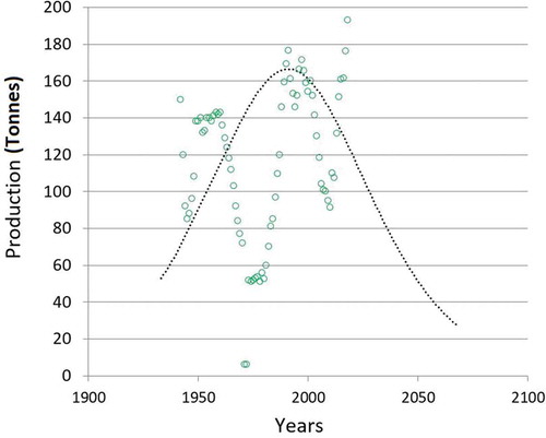
When the classic logistic curve created for gold production data is compared with the historic dataset of points, visible subsets are alternatively distributed in rising and falling trends above and below the Hubbert curve. This variance could be the determining factor to compensate or balance the uneven history of gold production in Canada, demonstrating a coincidence between the peak year indicated by the logistic curve, and the last reported one (1991) before 2018 (Cf. Wellmer & Scholz, Citation2016).

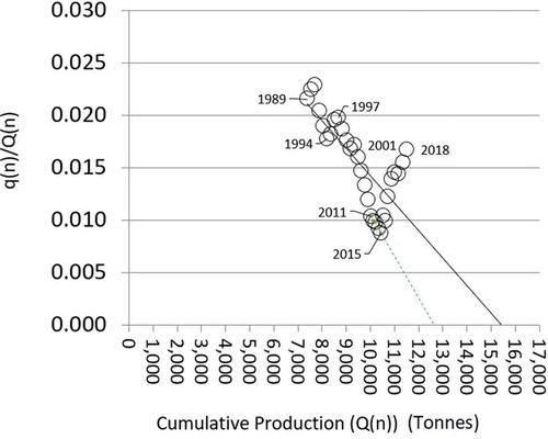
During the construction of the Hubbert model presented in Figure , an essential goal is to determine a range of initial reserves R₀ (equivalent to an estimated ultimate recovery (EUR), Q∞), with the assistance of the Hubbert’s linearization plot (Figure ). The plot illustrates an average value of 15,440 tonnes of ultimate reserves (black line), which could be considered as an optimistic one. If a conservative plot is obtained via a lower envelope line (green segmented line in the figure), made with a subset of border low-end distribution points (Karanki, Kushwaha, & Verma, Citation2009; Murtha, Citation1993), a figure of 12,600 tonnes results. In view of the, an average valuation that could be taken as a total mineral volume would be in the range of 14,000 tonnes. Alternatively, according to Drake (Citation2018), the official reserves are estimated as 11,403 tonnes. This calculation is derived from the addition of the 2010 official value of reserves (1,475 tonnes) plus the cumulative total production of 10,428 tonnes by December that year. The Hubbert linearization results indicate the need to review and upgrade this conservative estimation.

Figure 2. Gold mining in Canada. Hubbert’s linearization. Q(t) versus q(t)/Q(t) plot

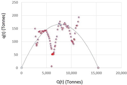
The EUR can be used with the production plot versus the cumulative production (Figure ), where the Hubbert linearization provides grounds to analyze the cumulative production as a quadratic function of the production (Deffeyes, Citation2006). In this instance, it is seen the extrapolation of the parabolic fit (blue curve and points) of a Hubbert curve-based distribution associated with an EUR of 15,400 tonnes. In a similar fashion to Figure , the red-blue points of the set of historic data of gold production are in sets scattered alternatively above and below respect to the ideal curve. The apex of the parabolic curve placed where the cumulative production equals half of the total reserves, matches the local peak of production achieved by 1991.

Figure 3. Gold mining in Canada. Plot of q(t) versus Q(t)

Having accomplished the reference goal for the total reserves or ultimate recovery, the next task is to figure an exact match between the historic data of Canada´s gold production and the concomitant distribution of points of the proposed model. This can be achieved by applying EquationEquation (4)(4) $q (n) = C (n) R (n - 1)$ (4) , considering the initial reserves as given by our estimate of Ro, and the model of the distribution with time of the PRR.

To illustrate the case, let’s examine in Figure the distribution of the PRR since the early forties of the 20^th century. It was constructed by the ratio between the yearly production outputs divided by the remaining reserves at the start of every year.

Figure 4. Gold mining in Canada. Distribution of PRR with time. Negative slope trends in green, moderately and high positive slope trends in brown and red, respectively

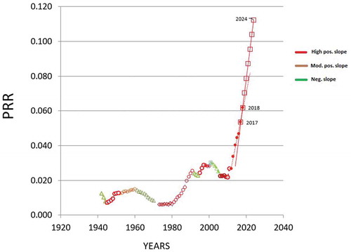
As stated by the definition of the remaining reserves, once a figure of initial reserves Ro is determined, they are calculated at every year by subtracting the cumulative production from Ro.

As seen in Figure , a piecewise model of the real PRR can be built as a succession of linear trends. High positive slope linear models (red points) of the PRR applies, as in the intervals of 1945 to 1951, 1978 to 1991. Moderate to low positive slopes linear models (brown points) are seen in the intervals from 1973 to 1980 or from 1952 to 1960. Negative slope linear models (in green) are appreciated during the early 1940s, the 1960s and from 2001 to 2007. There are no clear cases of a constant PRR with time, where EquationEquations (1)(1) $q (n) = C R o {(1 - C)}^{n - 1}$ (1) –(Equation3(3) $Q (n) = R o (1 - {(1 - C)}^{n})$ (3) ) could be applied to model production.

Let’s now proceed with the simulation to forecast the future trend of production.

To that end, it is sufficient to inspect the distribution of PRR with time for the last years of production. As seen in Figure , the points (red circles) from 2012 to 2018 result in a linear trend that could provide support for making a forecast based on applying EquationEquation (8)(8) $q (n) = C (n) R (n - 1) = C (n) R o (1 - C o) (1 - C (1)) . . (1 - C (n - 2))$ (8) . It is interesting to notice that if a line is built with 2015 and 2016, a backward match between the extrapolated values and the real ones of the previous years (down to 2012) can be verified.

However, for this case, the PRR of 2017 and 2018 will be used to build the equation and the linear trend (red squares and line). The reason is to account for the effect in the PRR of the discovery of fresh gold reserves in 2017 (Holmes, Citation2019), which created conditions for a clear increase of the slope of the PRR respect to the one for a distribution of points accounting the years prior to the discovery.

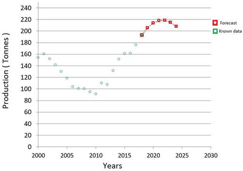
The distribution of recent (green points) and future production outputs (years 2019–2024, red squares and segment) is shown in Figure . The prediction is based on the linear extrapolation up to 2024 of the PRR line made from the 2017–2018 data as presented in Figure . It is seen that if the current linear trend of the PRR is kept during the next years, the production will likely reach successive record highs in excess of 200 tonnes, until a peak in the order or 220 tonnes will be achieved by 2022. However, if no new significant addition of reserves happens by then, by 2024 the production will fall to yields comparable to those seen by 2019.

Figure 5. Prediction of the gold production trend (years 2019–2024, red squares). Data of the historical record of recent production in green points

4. Discussion

The rising and falling subsets of historic records of gold production in Canada, although in clear departure from the ideal Hubbert model, seem to work out an overall balance that supports the coincidence between a real and a theoretical peak of production achieved by 1991, when the cumulative production amounted half of the total reserves diagnosed via the Hubbert linearization. The rudimentary fit between the ideal Hubbert curve and the real gold production in Canada points that a multi-Hubbert cycle analysis could offer a more suitable model than the one based on this traditional approach to reproduce the uneven historic record of the production of this mineral in Canada. The model of production provided by multi-Hubbert cycles would allow an upgraded recreation of the production as a result of the addition of inputs of factors that influence the mineral yields through time.

Comparing the initial reserves provided by the Hubbert´s linearization plot and the official values of reserves by Drake (Citation2018), there are evidences that the latter could underestimate the real amount of gold resources of Canada. This seems to be the case, since the estimation of reserves based on the Hubbert linearization or the q(t) vs Q(t) plot (Figure ) are in a range 10% to 35% higher than the official reserves, which were calculated in a traditional way from the collective contribution of appraised proven reserves of the gold mines in Canada.

The dissection of the formula of the Hubbert’s curve in the variables that define EquationEquation (12)(12) $q (n) = k Q (n) (1 - \frac{Q (n)}{R o}) = \frac{k Q (n)}{R o + k Q (n)} R o + k Q (n) (1 - \frac{Q (n)}{R o}) = C (n) \frac{R o^{2} - k Q {(n)}^{2} + R o (k - 1) Q (n)}{R o}$ (12) paves the way to understand the difference between the real and the ideal dynamic of mineral production.

One aspect that conditions the departure or coincidence of real profiles from the ideal Hubbert‘s curve lies on the differences or correspondences of the distribution with time of the PRR.

If the PRR of the real profile of production does not follow the expression given in EquationEquation (11)(11) $C (n) = \frac{P (n)}{R (n - 1)} = \frac{P (n)}{R (n) + P (n)} = \frac{k Q (n) (1 - \frac{Q (n)}{R o})}{R o + k Q (n) (1 - \frac{Q (n)}{R o})} = \frac{k Q (n)}{R o + k Q (n)}$ (11) , differences between the real trend of production and the Hubbert ideal curve will ensue.

The other aspect that set up the coincidence or difference between the real trend of production and the Hubbert ideal curve is whether or not the PRR equals EquationEquation (11)(11) $C (n) = \frac{P (n)}{R (n - 1)} = \frac{P (n)}{R (n) + P (n)} = \frac{k Q (n) (1 - \frac{Q (n)}{R o})}{R o + k Q (n) (1 - \frac{Q (n)}{R o})} = \frac{k Q (n)}{R o + k Q (n)}$ (11) and the distribution of reserves with time follows the quadratic factor present in the right member of EquationEquation (12)(12) $q (n) = k Q (n) (1 - \frac{Q (n)}{R o}) = \frac{k Q (n)}{R o + k Q (n)} R o + k Q (n) (1 - \frac{Q (n)}{R o}) = C (n) \frac{R o^{2} - k Q {(n)}^{2} + R o (k - 1) Q (n)}{R o}$ (12) .

In effect, from the comparison of EquationEquations (11)(11) $C (n) = \frac{P (n)}{R (n - 1)} = \frac{P (n)}{R (n) + P (n)} = \frac{k Q (n) (1 - \frac{Q (n)}{R o})}{R o + k Q (n) (1 - \frac{Q (n)}{R o})} = \frac{k Q (n)}{R o + k Q (n)}$ (11) , (Equation12(12) $q (n) = k Q (n) (1 - \frac{Q (n)}{R o}) = \frac{k Q (n)}{R o + k Q (n)} R o + k Q (n) (1 - \frac{Q (n)}{R o}) = C (n) \frac{R o^{2} - k Q {(n)}^{2} + R o (k - 1) Q (n)}{R o}$ (12) ) and (Equation4(4) $q (n) = C (n) R (n - 1)$ (4) ) it follows that the FEMP coincides with the Hubbert curve if C(n) follows the function given by EquationEquation (11)(11) $C (n) = \frac{P (n)}{R (n - 1)} = \frac{P (n)}{R (n) + P (n)} = \frac{k Q (n) (1 - \frac{Q (n)}{R o})}{R o + k Q (n) (1 - \frac{Q (n)}{R o})} = \frac{k Q (n)}{R o + k Q (n)}$ (11) and also:

(14)

R (n - 1) = \frac{R o^{2} - k Q {(n)}^{2} + R o (k - 1) Q (n)}{R o}

(14)

With EquationEquations (12)(12) $q (n) = k Q (n) (1 - \frac{Q (n)}{R o}) = \frac{k Q (n)}{R o + k Q (n)} R o + k Q (n) (1 - \frac{Q (n)}{R o}) = C (n) \frac{R o^{2} - k Q {(n)}^{2} + R o (k - 1) Q (n)}{R o}$ (12) and (Equation14(14) $R (n - 1) = \frac{R o^{2} - k Q {(n)}^{2} + R o (k - 1) Q (n)}{R o}$ (14) ), the grounds to investigate the equivalence between the Hubbert model and the general expression of the FEMP (EquationEquation (4)(4) $q (n) = C (n) R (n - 1)$ (4) have been found. In this sense, the compliance of the Hubbert model with the LCM would be warranted, as far as the distribution of reserves in this model observes the identity featured by EquationEquation (14)(14) $R (n - 1) = \frac{R o^{2} - k Q {(n)}^{2} + R o (k - 1) Q (n)}{R o}$ (14) , which was derived from an expression constructed following the LCM (EquationEquation (10)(10) $R (n - 1) = R (n) + P (n) = R o - Q (n) + P (n) = (R o - Q (n)) (1 + \frac{k Q (n)}{R o}) = (R o + k Q (n)) (1 - \frac{Q (n)}{R o})$ (10) ).

A crucial result of the comparative study between the Hubbert model and the general expression of the FEMP (EquationEquation (4)(4) $q (n) = C (n) R (n - 1)$ (4) ), is that the coincidence between them occurs when the PRR of the FEMP coincides with that of the Hubbert model (EquationEquation (10)(10) $R (n - 1) = R (n) + P (n) = R o - Q (n) + P (n) = (R o - Q (n)) (1 + \frac{k Q (n)}{R o}) = (R o + k Q (n)) (1 - \frac{Q (n)}{R o})$ (10) ), which is nonlinear.

Coming back to the FEMP, from EquationEquation (4)(4) $q (n) = C (n) R (n - 1)$ (4) it is inferred that the production can be envisioned as a composite function of the distribution with time of the reserves and the PRR.

Provided that the change of the reserves with time depends only on the successive subtractions of production yields from a known initial volume of them, the focus on the analysis of EquationEquation (4)(4) $q (n) = C (n) R (n - 1)$ (4) would rest on the behavior of the PRR through time. Of special interest in this matter would be the projection of the trend of the PRR component of the fundamental equation to forecast future outputs of mineral production.

In the case examined, although the PRR displays a consistent positive linear trend during almost a decade, it was considered most appropriate to use the two very last years after the finding of nearly 800 tonnes of new gold reserves in British Columbia in 2017 to make the forecast analysis. The effect in the increase of the PRR of the sudden availability of such whooping amount of reserves deserved such a treatment. Had this fortuitous discovery not been made, a larger set of points could easily be used to make the linear extrapolation that supported the forecast made.

There are possibilities for uncontrolled effects of variables not included in the FEMP that could significantly alter patterns of production. Examples include discoveries of massive mineral accumulations (several hundreds of tonnes) of relatively easy short-term development, that could increase the reserves and the PRR in a fashion not foreseeable before such findings, or technological breakthroughs that could increase the reserves and the PRR out of resources at hand but previously uneconomical to develop, as happened with the shale oil and gas revolution during the last decade. The effect on mine production (and on the PRR) of some factors, like economic growth of regional markets can be reviewed with the results found and serve as a reference for possibilities of their influence in shaping future trends. For instance, the sharp increase in the PRR and of production during the 1980s (Figures and ) is in accord not only with the new reserves available to develop in the country through the massive discovery at Hemlo (Ontario) in the early 1980s (Barnes, Citation1995; Colvine, Citation1983) but also with a global economic trend attributed to a response for rise in gold demand from Asian markets during that time (Wiggins, Citation2003).

Other examples but in the opposite direction could be mismanagements or disruptions of mineral development plans leading to falls in production not in agreement with availability of the resource, as has recently been seen in the oil production of Venezuela since 2016, or during the 1990s in Kuwait right after the invasion by Iraq. The influence of factors like these, which depend upon on political scenarios, has the caveat that for social sciences it has been shown that there is only a short time span for reliable predictions of future events (Tetlock, Citation2013). One way to handle such scenarios could be to make probabilistic forecasts considering wide ranges of production that for countries with a record of political instability could embrace such extreme possibilities.

However, an in deep interpretation of the meaning of the patterns of the PRR with time in terms of several factors other than addition of reserves (economic, political or social stress) is still pending to be analyzed. It is left for future studies and further development of the proposals introduced in the present work.

The meaning of the patterns of the PRR with time in terms of several factors (economic, political, social stress or the lack of it) is still to be analyzed. It is left for future studies and further development of the proposals introduced in the present work.

One interesting aspect to consider about the use of the plot of the PRR for forecasting is that only two consecutive initial points of a trend would suffice to identify the line that would regulate the production for the next years. For instance, in Figure it is seen that the linear trend given by the set of PRR for 2010 to 2011 would suffice to predict the PRR for the following next six years of known production rates. The plot in Figure shows that the linear trends of positive slope have run for as long as a dozen of years (as for the interval 1980–1991) or as short as for three years (as for the interval 1995 to 1997). One crucial guideline to decide whether or not to extrapolate a linear trend of positive slope beyond the three years threshold seems to be a fair estimation of the continuity or not of the conditions supporting such linear increase of the PRR with time.

Analysts using means of forecasting other than the FEMP (Galbraith, Citation2019; Holmes, Citation2019; Mining Technology, Citation2019) coincide with a near term prediction of steady increase of production in Canada as the one made in base of the trend of the latest linear of the PRR. These independent examinations support a fast-national growth of gold production in Canada that is expected to last for several years, with continued ramp-up and additional startups in Nunavut Territory, northern Quebec, British Columbia and Nova Scotia. With these developments is expected to be a more than satisfactory compensation of the decline from mines in Manitoba, Saskatchewan and the Yukon (Mining Technology, Citation2019; NRCAN, Citation2019). In the short-term Canada is likely to become the fourth-largest gold-producing country at global scale, passing the U.S. in national gold production (Galbraith, Citation2019). Although the analysis made with the FEMP shows the reaching of a peak in the order of 220 tonnes by the mid-2020s, there has been at least one more optimistic prediction pointing that the heavy flow in the exploration sector provides grounds for Canada to reach 300 tonnes of annual gold production by this same time (Jamasmie, Citation2018).

Among the multiple directions for future research it can be mentioned comparative studies between the FEMP and predictive models other than the Hubber curve, like Decline Curve Analysis (DCA, Ilk, Rushing, Perego, & Blasingame, Citation2008) or time series analysis (Elliot & Timmermann, Citation2016; Goodwin, Citation2015; Makridakis, Wheelwright, & Hyndman, Citation2008; Selvanathan & Selvanathan, Citation2003). The incorporation of the FEMP as a resource in Machine Learning algorithms dedicated to the modeling and forecasting of mineral production is also a subject for future investigations (Cf. Tamimi, Samani, Minaei, & Harirchi, Citation2019). A combination of the aforementioned with revisions to figure key predictor variables besides the ones considered in the EMP to account with in the forecast of mineral production (Elliot & Timmermann, Citation2016) will help to concentrate in the effects of those aspects of the universe of information that are critical rather than nonessential for prediction purposes (Gigerenzer, Citation2013). Other subjects to be mentioned are There are significant options of research streaming from the robust foundation of the FEMP on the LCM. Among them, there are ongoing projects about a transition of the equation from mineral production into subjects of operational research (modeling of work production), theoretical physics contemplated in the theory of conservation of energy (Yuhua, Citation2014) and in material flow analysis (Brunner & Rechberger, Citation2017).

5. Conclusions

The overall picture provided by the traditional Hubbert curve applied to model gold production in Canada suffices to identify the EUR, a historic peak of production correlative with the depletion of half of the reserves, and the likely current degree of exploitation of the resource. However, a multi-Hubbert model could provide a more comprehensive grasp of the uneven record of production of the mineral than the basic model given by the traditional approach.

The study of gold reserves in Canada via the Hubbert´s linearization indicates the official account of reserves underestimates in a likely range from 10% to 35% the real amount of gold resources of the country.

A piecewise discrete version of the FEMP where the PRR can be discretized in linear segments is introduced. This presents a complementary resource to the FEMP based on a constant PRR to model mineral production when the PRR is not constant but changes with time.

The results presented offer the conditions of equivalence between Hubbert’s formulation and the FEMP. The formula of the Hubbert’s curve of production can be divided into the contribution of the distribution with time of the remaining reserves and the PRR, the two variables considered in the FEMP.

The general capability of the FEMP to model historic profiles of production, however complex, relies on fitting the distribution with time of the PRR, as an independent variable, to an adequate linear or nonlinear trend. This provides a viable alternative to skip the discrepancies between real production profiles and ideal models of production with symmetrical curves.

The fundamental equation considers the variations of the PRR with time and addresses the issues of the real dynamics of mineral production. The factors affecting the dynamics, disregarding what they could be, are truly reflected in the PRR.

The advantage of the FEMP respect to ideal models, like the classic Hubbert curve or those empirically derived like the ones of DCA, is that it is built upon the LCM, which enables it to model complex patterns of mineral production, however complex, with a faithful reproduction of its features under the frame of a natural law.

A unique differentiator of the FEMP from other models is the identification and study of the distribution of linear patterns in the PRR with time. The study of these linear patterns facilitates insights about the causes behind definite trends followed by mineral production during the intervals of time investigated. This has a significant impact in the understanding of the process modelled, which provides a significant contribution to the methodologies in use in this field of research.

The analysis of the trend posed by the last years of the PRR is vital to extrapolate its behavior in the future and to predict the production using the FEMP.

In the case of gold mining in Canada, the linear trend of positive slope displayed by the PRR of this activity during recent years shows that unless there is another significant increase of fresh reserves by new discoveries and/or the influence of global economic factors, leading to a rise the gradient of the linear function of the PRR, the output of the metal will continue to reach ever-increasing peaks until an all-time record high is to be achieved by the mid of the next decade.

Acknowledgements

To my patroness and patrons for the favors received during the progress of this project, especially during July 15 and 11, respectively.

To my wife and daughters for their care, company and understanding of the sacrifices of solitude work.

Additional information

Funding

The author received no direct funding for this research.

Notes on contributors

Sergio Pérez Rodríguez

Sergio Perez Rodriguez works as a Field Researcher in the Energy & Natural Resources division of a London-based data and analytics firm. Prior to that he was a Basin Researcher for the same company, committed for a half-decade to do intelligence analysis for exploration of sedimentary basins in Latin America. Among other projects in geoscience, it has been dedicated to innovation in the modeling and forecast of mineral production through the conception and development of the Equations of Mineral Production, one of the topics of research whose results has divulged during the last decade and a half in several journals and conferences. Sergio has a degree in Engineering Geology by the Universidad Central de Venezuela, and a Postgraduate Diploma in Geology and a Master in Science, both granted by Royal Holloway, University of London.

References

24hgold.com. (2019). Statistics: All countries. 24hgold.com. Retrieved from http://www.24hgold.com/english/stat_all_countries.aspx
Google Scholar
Barnes, M. (1995). Gold in Ontario. Boston: Boston Mills Press.
Google Scholar
Bertrand, M. (2011). Oil production: A probabilistic model of the Hubbert curve. Applied Stochastic Models in Business and Industry, 27(4), 434–16. doi:10.1002/asmb.851
Web of Science ®Google Scholar
Brunner, P. H., & Rechberger, H. (2017). Handbook of material flow analysis: For environmental, resource, and waste engineers. Boca Raton: CRC Press LLC.
Google Scholar
Claerbout, J., & Muir, F. (2008). Hubbert math. Sepstanford.edu. Retrieved from http://sepwww.stanford.edu/sep/jon/hubbert.pdf
Google Scholar
Colvine, A. C. (1983). The geology of gold in Ontario. Ontario: Ontario Ministry of Natural Resources.
Google Scholar
Deffeyes, K. (2006). Beyond oil. The view from Hubbert’s. Peak: Hill and Wang.
Google Scholar
Drake, A. (2018). Canadian reserves of selected major metals and recent production decisions. Natural Resources Canada. Nrcan.gc.ca. Retrieved from https://www.nrcan.gc.ca/mining-materials/exploration/8294#t2
Google Scholar
Elliot, G., & Timmermann, A. (2016). Economic forecasting. Princeton: Princeton University Press.
Google Scholar
Evans, G., & Mohr, S. (2010, October 10). The generalized Hubbert curve. The Oil Drum. Retrieved from http://theoildrum.com/node/7072
Google Scholar
Galbraith, C. (2019). 2019 gold output to hit new record high of 109.6 Moz. S&P Global. Market Intelligence. Retrieved from https://www.spglobal.com/marketintelligence/en/news-insights/trending/zhSggm-ztc-nJuneeXr2dQ2
Google Scholar
Gigerenzer, G. (2013). Smart heuristics. In J. Brockman (Ed.), Thinking: The new science of decision-making, problem-solving, and prediction (pp. 39–54). New York, NY: Harper.
Google Scholar
Goodwin, N. (2015). Bridging the gap between deterministic and probabilistic uncertainty quantification using advanced proxy based methods. SPE Reservoir Simulation Symposium 2015 (Vol. 3, pp. 1796–1868). New York, NY: Curran Associates.
Google Scholar
Holmes, F. (2019). Top 10 gold producing countries. U.S. Global Investors. Insight for Investors. Retrieved from http://www.usfunds.com/investor-library/frank-talk/top-10-gold-producing-countries/#.XgvOH_x7nRZ
Google Scholar
Höök, M., Davidsson, S., Johansson, S., & Tang, X. (2014). Decline and depletion rates of oil production: A comprehensive investigation. Philosophical Transactions of the Royal Society A, 372, 20120448. doi:10.1098/rsta.2012.0448
Web of Science ®Google Scholar
Hubbert, M. K. (1982). Techniques of prediction as applied to production of oil and gas. NBS special publication. US Department of Commerce, 631, 1–121.
Google Scholar
Ilk, D., Rushing, J. A., Perego, A. D., & Blasingame, T. A. (2008). Exponential vs. hyperbolic decline in tight gas sands — Understanding the origin and implications for reserve estimates using arps’ decline curves. SPE 116731. SPE Annual Technical Conference and Exhibition, Denver, CO, ATCE 2008 (Vol. 7, pp. 4637–4659). New York, NY: Curran Associates.
Google Scholar
Jamasmie, C. (2018). GOLD: Canada could be world’s second biggest gold producer. Canadian Mining Journal News. Retrieved from http://www.canadianminingjournal.com/news/gold-canada-worlds-second-biggest-gold-producer/
Google Scholar
Karanki, D., Kushwaha, H., & Verma, A. (2009). Uncertainty analysis based on probability bounds (p-box) approach in probabilistic safety assessment. Risk Analysis, 29, 662–675. doi:10.1111/j.1539-6924.2009.01221.x
PubMed Web of Science ®Google Scholar
Makridakis, S., Wheelwright, S. C., & Hyndman, R. J. (2008). Forecasting methods and applications (3rd ed.). New Delhi: Wiley India.
Google Scholar
Mining Technology. (2019). Canada’s gold production to reach 7.6Moz by 2023. Comments. Retrieved from https://www.mining-technology.com/comment/canadas-gold-production/
Google Scholar
Mohr, S. H., & Evans, G. M. (2010). Combined generalized Hubbert-Bass model approach to include disruptions when predicting future oil production. Natural Resources, 1(1), 28–33. doi:10.4236/nr.2010.11004
Google Scholar
Murtha, J. A. (1993). Decisions involving uncertainty – An @Risk tutorial for the petroleum industry. Newfield: Palisade Corporation.
Google Scholar
NRC- National Research Council. (2008). Minerals, critical minerals, and the U.S. economy. Washington, DC: National Academies Press.
Google Scholar
NRCAN- Natural Resources Canada. (2019). Gold Facts. Minerals and Metals Facts. Retrieved from https://www.nrcan.gc.ca/our-natural-resources/minerals-mining/minerals-metals-facts/gold-facts/20514
Google Scholar
Patzek, T. W. (2008). Exponential growth, energetic Hubbert cycles, and the advancement of technology. Archives of Mining Sciences, 53(2), 131–159.
Web of Science ®Google Scholar
Patzek, T. W., & Croft, G. D. (2010). A global coal production forecast with multi-Hubbert cycle analysis. Energy, 35, 3109–3122. doi:10.1016/j.energy.2010.02.009
Web of Science ®Google Scholar
Pérez Rodriguez, S. (2013a). Methodology and equations of mineral production forecast. Part I. Crude oil in the UK and Gold in Nevada, USA. Prediction of late stages of production. Open Journal of Geology, 3, 352–360. doi:10.4236/ojg.2013.35040
Google Scholar
Pérez Rodriguez, S. (2013b). Methodology and Equations Of Mineral Production Forecast. Part II. The fundamental equation. Crude oil production in USA. Open Journal of Geology, 3, 384–395. doi:10.4236/ojg.2013.36044
Google Scholar
Pérez Rodriguez, S. (2018). Lessons learned from a shale gas hallmark well in the eagle ford formation: The Case of the emergente–1 well, the first shale gas well in Mexico. Gulf Coast Association of Geological Societies Transactions, 68, (pp.747).
Google Scholar
Roper, L. D. (1976). Where have all the metals gone? Blacksburg, Virginia: Virginia Polytechnic Institute and State University. Retrieved from http://www.roperld.com/science/minerals/metalgon.pdf
Google Scholar
Saraiva, T., Szklo, A., Lucena, A., & Chavez-Rodriguez, M. (2014). Forecasting Brazil’s crude oil production using a multi-Hubbert model variant. Fuel, 115(1), 24–31. doi:10.1016/j.fuel.2013.07.006
Web of Science ®Google Scholar
Selvanathan, S., & Selvanathan, E. A. (2003). Gold production in Western Australia. In M. Tcha (Ed.), Gold and the modern world economy (pp.161–188). London: Routledge.
Google Scholar
Tamimi, N., Samani, S., Minaei, M., & Harirchi, F. (2019). An artificial intelligence decision support system for unconventional field development design. Proceedings of the 7th Unconventional Resources Technology Conference 2019 (pp. 503–513). Tulsa: SEG. doi:10.1177/1753193419826486
Google Scholar
Tetlock, P. (2013). How to win at forecasting. In J. Brockman (Ed.), Thinking: The new science of decision-making, problem-solving, and prediction (pp. 18–38). New York, NY: Harper.
Google Scholar
US HCNR-United States. Congress. House. Committee on Resources. Subcommittee on Energy and Mineral Resources. (2003). The role of strategic and critical minerals in our national and economic security: Oversight hearing before the Subcommittee on energy and mineral resources of the committee on resources, U.S. house of representatives, one hundred eighth congress, first session, Thursday, July 17, 2003. Washington, DC: U.S. G.P.O.
Google Scholar
Vaccari, D. A., Mew, M., Scholz, R. W., & Wellmer, F. W. (2014). Exploration: What reserves and resources? In R. W. Scholz, A. H. Roy, F. S. Brand, D. T. Hellums, & A. E. Ulrich (Eds.), Sustainable phosphorus management: A global transdisciplinary roadmap (pp. 129–151). Dordrecht: Springer.
Google Scholar
Wellmer, F. W., & Scholz, R. W. (2016). Peak minerals: What can we learn from the history of mineral economics and the cases of gold and phosphorus? Mineral Economics, 30(2), 79–93.
Web of Science ®Google Scholar
Wiggins, C. (2003). Western Australia commodity outlook: Gold. In M. Tcha (Ed.), Gold and the modern world economy (pp.8–18). London: Routledge.
Google Scholar
Wright, S. (2013). Global gold-mining trends 3. Zealllc.com. Retrieved from http://www.zealllc.com/2013/ggmt3pf.htm
Google Scholar
Yuhua, F. (2014). Unified theory of natural science so far and FTL problems. In F. Smarandache (ed.). Proceedings of the First International Conference on Superluminal Physics & Instantaneous Physics as New Fields of Research (pp. 58–82). Columbus: Education Publisher.
Google Scholar

Modeling and forecasting complex patterns of mineral production. Gold mining in Canada