An optimization model of make or buy decision and quality improvement of components using rebate

Abstract

The aim of this research is to develop a make or buy decisions optimization model involving rebate for quality improvement to minimize a total cost comprising of manufacturing cost, quality loss, and lateness cost by taking into consideration the process capability, production capacity, supplier capacity, costumer demand, due date, and process routing. Several constraints are imposed in the model include tolerance limits, process variance of the components, minimum number of the selected machine or supplier, and the quality level before and after rebate. A numerical example is given to show the application of the model. The optimization results show that the inclusion of the rebate to the model gives benefits to the system by improving the quality and reducing the quality loss. From the analysis, prevention cost has the most significant impact on suppliers total cost.

Keywords:

• make or buy
• optimization
• quality improvement
• rebate
• tolerance

PUBLIC INTEREST STATEMENT

This paper discusses the decisions that must be made in a manufacturing company concerning several important issues. First, how to determine simultaneously which component should be made in-house and which ones must be outsourced along with the respective allocation of the components. Second, how the company improve the quality of components using rebates especially for the components purchased from the suppliers. The paper shows that rebates consider as an effective way to improve the quality of components through process improvements in suppliers side. Three quality costs are considered in this paper, namely prevention cost, appraisal cost, and failure cost. Among those costs, prevention cost give the most significant impact on the total cost of suppliers.

1. Introduction

Manufacturing companies have to set appropriate strategies to win the competition in a competitive market. According to Porter (1980), business strategy is needed by a company in order to be competitive in the market. There are three factors affecting the business strategy of the company, namely quality improvement, cost reduction, and on-time delivery (Hallgren & Olhager, 2006). Quality improvement deals with reducing the product or component variance (Ding et al., 2000). Higher product or component variance will result in lower quality. Hence, the company has to maintain and even improve its product quality by reducing the variance.

Improving quality of a product or component is not an easy task. Hence, a proper tolerance design is necessary to control the variance of the product (Mustajib & Irianto, 2010). Tolerance serves to limit the variability around the product quality characteristics target. According to Zhang (1996), tolerance is a critical issue in product and process design stage, since it will become the connector between product requirement and manufacturing cost. The tighter the tolerance of a component, the higher the manufacturing cost, and conversely the looser the tolerance of a component the lower the manufacturing cost (Chase et al., 1990). Quality loss will be incurred when product quality does not conform to the predetermined quality target. Therefore, quality improvement has to be performed continuously by reducing the variance of the product (Harrington, 1987).

The last factor of competitive strategy is on-time delivery where the company should deliver the orders on time, since the lateness will have a negative impact on costumer’s satisfaction. There will be an opportunity loss due to unsatisfied customers in the form of the number of orders received by the company. The lateness can be minimized using an appropriate production scheduling, so all orders can be completed and delivered to customers on time.

To satisfy customer demand, the company has three alternative policies, namely in-house production (make), outsourcing (buy), or mixed between make and buy. According to Rosyidi et al. (2014), there are three main factors that must be considered in make or buy decisions, namely production capacity, process capability, and technological capability. Production capacity deals with the ability to fulfill the quantity of demand. Process capability is the measure of a process to achieve component or product specifications, while technological capability deals with the ability to produce certain type of components.

Outsourcing is not a simple activity since it deals with critical decision making to determine appropriate suppliers from whom the components should be purchased (Teeravaraprug, 2008). Banaeian et al. (2015) pointed that supplier selection is a very crucial decision for company performance. Uncertainty in term of supply, process, and demand make the outsourcing even more complex (Angkiriwang et al., 2014). Subramanian et al. (2014) summarized that outsourcing complexity mainly deals with the interaction of system members and will have an impact on the transaction costs, supply risk, supplier responsiveness, and supplier innovation.

In suppliers selection, one of manufacturer concerns deals with the problems of components quality level in terms of both yield and quality cost (Montgomery, 2001). Within the scope of supply chain, both manufacturer who delivers the final product to customer and suppliers who supply components to manufacturer, have a significant impact on the product quality level (Kusukawa et al., 2006). The improvement of quality components will reduce the total cost and increases the efficiency of supply chain.

In current practice, make or buy decisions do not only deal with determining which components must be purchased from the suppliers, but also deal with determining the suppliers for certain production or manufacturing processes (Bardhan et al., 2006; Maia et al., 2015). According to the survey conducted by Peerless Research Group (2016), the majority (84%) of organizations outsource their production to some extent. There are two main reasons for this outsourcing: reduce manufacturing costs and the need for manufacturer to increasingly focus on their core competencies. Hence, the company has to outsource part or all of their manufacturing operations to third-party manufacturers (subcontractors) (Sousa & Voss, 2007).

Make or buy analysis and quality improvement has attracted many researchers. Mustajib and Irianto (2010) developed an integrated model for process selection and quality improvement in a multistage process production. Teeravaraprug (2008) formulated a model of outsourcing and vendor selection based on Taguchi loss function. Oncu et al. (2003) presented make or buy analysis using analytical hierarchy process for local manufacturer and import decision procurement system in Turkey. Duarte et al. (2016) presented a dynamic optimization strategy to formulate and solve the problem to find the optimum quality improvement for a given company. The problem was characterized by the level of quality and the efficiency of transforming investment into tangible quality improvements using in prevention-appraisal-failure (PAF) approach. Rosyidi et al. (2016a) developed a process selection model to minimize manufacturing cost, quality loss, and lateness cost. The model is then extended by considering multistage manufacturing processes, quality improvement efforts involving learning and forgetting curve, and equipment investment and profit sharing (Rosyidi et al., 2014, 2016b; Pratama et al., 2018; Rosyidi & Pratama, 2018; Sofiana et al., 2019)

Those above research dealt with the development of make or buy analysis and quality improvement models without taking into consideration the component quality improvement. Several strategies can be used in quality improvement. For example, quality investment can be used as a strategy to improve component quality produced both in-house and outsource. Rosyidi et al. (2016c; 2016d) developed optimization models using this strategy to determine optimal learning investments. Another strategy in quality improvement is by giving some incentives to the respective managers as developed by Veldman and Gaalman (2014). The incentive is also important for suppliers to increase their effort in quality improvement. Using this strategy, Kusukawa et al. (2006) developed an optimization model in the form of profit sharing which known as rebate.

The model in this paper is developed based on the research of Rosyidi et al. (2016b) and Kusukawa et al. (2006). The former research deals with process/suppliers selection and component allocation to the selected process/suppliers. The later deals with how to improve the quality of components that purchased from the suppliers. Hence, the later research implicitly assumed that all the needed components are outsourced, while in real world there are many companies not outsourced all their needed components. Hence, at least three contributions are given by this paper. First, it helps the decision makers in making important decisions about design and manufacturing simultaneously. Second, the quality improvement decisions are also determined from the model, mainly for the outsourced component through rebates. Third, the model consider scheduling decisions which will minimize the production lead time and hence reduce the product delivery lateness. Furthermore, the analysis about rebates must be made earlier along with the make or buy analysis so the manufacturer knows how the rebates will affect the total cost and components allocation. Hence, the aim of this research is to develop a make or buy decision model considering quality improvement with rebate to minimize a total cost comprising of manufacturing cost, quality loss, and lateness cost. The model will help a manufacturer in making decisions concerning make or buy and the order allocation to determine optimum rebate for related suppliers who exceeds the target quality set by the manufacturer. Table 1 shows the position of this research relative to other relevant research.

Table 1. Position of the proposed model

Researchers	Process stage		Suppliers		Process selection	Supplier selection	Component allocation	Quality improvement
	Single	Multi	Single tier	Multi tier				Learning investment	Rebates
Kusukawa et al. (2006)	X	√	X	√	X	X	X	X	√
Rosyidi et al. (2014)	√	X	√	X	√	√	X	X	X
Rosyidi et al. (2016a)	√	X	√	X	√	√	X	X	X
Rosyidi et al. (2016b)	X	√	√	X	√	√	√	X	X
Rosyidi and Pratama (2018)	X	√	√	X	√	√	√	√	X
Pratama et al. (2018)	X	√	√	X	√	√	√	√	X
Sofiana et al. (2019)	√	X	X	√	X	X	X	√	√
This research	X	√	X	√	√	√	√	X	√

2. Model development

2.1. Notations

I	=	Component index, i = 1,2, …,I
J	=	Supplier index, j = 1,2, …, J
M	=	Machine index, m = 1,2, …, M
k	=	Stage index, k = 1,2, …, K
h	=	Predecessor supplier index, h = 1,2, …, H
Mimk	=	Manufacturing cost of component i in machine m at stage k
ximk	=	Allocation of component i in machine m at stage k
bimk	=	Binary of component i in machine m at stage k
cij	=	Manufacturing cost of component i at supplier j
xij	=	Allocation of component i at supplier j
bij	=	Binary of component i at supplier j
A	=	Coefficient of quality loss
TR	=	Assembly tolerance limit
σA2	=	Assembly variance
qh*	=	Optimum quality level of supplier h before rebate
qh**	=	quality level of supplier h after rebate
qj*	=	Optimum quality level of supplier j before rebate
qj**/	=	Optimum quality level of supplier j after rebate
Lhj	=	Failure cost of supplier j received from supplier h
mj	=	Prevention cost of supplier j
dj	=	Appraisal cost of supplier j
rj	=	Total quality level impact at supplier j
ᴷj	=	Variable remuneration of supplier j
Uj	=	Fix remuneration of supplier j
D	=	Demand of final product
E(S)asm	=	Expected scrap in assembly process
E(S)com	=	Expected scrap in manufacturing process
SCasm	=	Scrap cost per unit product in assembly process
SCcom	=	Scrap cost per unit product in manufacturing process
y	=	Lateness time
L	=	Lateness cost
TC	=	Expected total cost
$\frac{\delta R}{\delta xi}$	=	Partial derivative equation of component i functional dimension
$t_{imk}$	=	Tolerance of component i in machine m at stage k
$t_{ij}$	=	Tolerance of component i from supplier j
Cp	=	Process capability index
kim	=	Production capacity of component i in machine m
kij	=	Production capacity of component i in supplier j
${\sigma }_{zi}^2$	=	Variation of stock removal of component i
${\sigma }_{\delta i}^2$	=	Variance of processing component i
$s_{imk}^b$	=	Production starting time for component i in machine m, stage k, and sequence b
$s_{imk}^a$	=	Production starting time for component i in machine m, stage k, and sequence a
$p_{imk}^a$	=	Processing time of component i in machine m, stage k, and sequence a
$C{S}^{\ast }$	=	Total cost of all suppliers before setting rebate
$C{S}^{\ast \ast }$	=	Total cost of all suppliers after setting rebate
$W$	=	Total time production
$w_{max}$	=	Total completion time of manufacturing process
$w_{ass}$	=	Total assembly time
$W_T$	=	Due date

2.2. System description

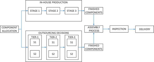
In this paper, we consider a system consists of single manufacturer with multi-tier suppliers. The manufacturer produces an assembly product in which the components are provided in-house and/or outsourced. Figure 1 shows the system considered in this paper.

Figure 1. The systems of the developed model.

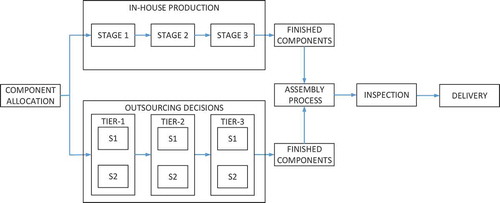
In making decision, the components are manufactured in multistage processes. Each type of component has different process routing. The manufacturer has several production stations in which each station has identical machines with different characteristics in term of tolerance, manufacturing cost, and processing time. Each machine has certain process capability and production capacity which will constrain the allocation decision in manufacturing process. In buy decision, the manufacturer performs supplier selection and component allocation to the selected suppliers. The outsourcing involves multitiers suppliers in which each supplier has capability to process the needed components. Each supplier has the same opportunity to supply the component and has different characteristics in term of tolerance, manufacturing cost, and processing time.

Predecessor supplier represents the first-tier supplier provides semifinished components to a subsequent supplier in the second tier. The last-tier suppliers deliver the finished components to the manufacturer. Each supplier has its own quality level with two quality costs, namely failure and appraisal costs. Subsequent suppliers incur not only failure cost due to the quality level in their own process, but also the failure cost from the quality level at the process of related predecessor supplier. If a predecessor supplier performs quality improvement on a certain component process, then it will increase the component quality level at subsequent supplier. Due to the efforts in quality improvement by each supplier then if the quality level of each supplier exceeds certain quality standard denoted by T and set by the manufacturer, then each respective supplier will receive a rebate from the manufacturer or subsequent supplier.

2.3. Rebates model

The rebates model used in this paper is taken from the research of Kusukawa et al. (2006). Their paper includes several costs such as failure and appraisal cost which resulted from outsourcing processes. The model calculates all of suppliers quality loss. In this research, Equations (1)(1) $C_{hj}\left(q_j\right)=x_{ij}{\sum }_{hϵS}\left(1-q_h\right)l_{hj}$(1) –(15) are taken from Kusukawa et al. (2006). Equation (1)(1) $C_{hj}\left(q_j\right)=x_{ij}{\sum }_{hϵS}\left(1-q_h\right)l_{hj}$(1) expresses the failure cost of each supplier. Subsequent suppliers incurs not only failure cost of the quality level of their own process, but also a part of failure cost caused by quality level at the process of the related predecessor suppliers.

(1) $C_{hj}\left(q_j\right)=x_{ij}{\sum }_{hϵS}\left(1-q_h\right)l_{hj}$(1)

In this paper, prevention and appraisal costs are considered as a single cost referred to as appraisal cost. Equation (2)(2) $C_{hj}\left(q_j\right)=m_j^{\frac{qj}{rj}}+d_j$(2) expresses the appraisal cost incurred by each supplier. When the predecessor suppliers perform quality improvement, then the appraisal cost of subsequent suppliers will decrease, due to the decrease of component inspection cost.

(2) $C_{hj}\left(q_j\right)=m_j^{\frac{qj}{rj}}+d_j$(2)

In this paper, the rebate will be determined by the quality level. If a supplier is able to increase the quality level and exceed the predetermined quality standard set by the manufacturer, then the supplier will receive rebate from the manufacturer. Equation (3)(3) $R_j\left(q_j\right)=\left\{\begin{array}{c}{\kappa }_j\left(q_j-T_j\right)+U_j,\left(q_j\ge T_j\right)\\ 0,\left(q_j<T_j\right)\end{array}\right.$(3) shows the formulation of the rebate.

(3) $R_j\left(q_j\right)=\left\{\begin{array}{c}{\kappa }_j\left(q_j-T_j\right)+U_j,\left(q_j\ge T_j\right)\\ 0,\left(q_j<T_j\right)\end{array}\right.$(3)

The optimum quality level at a supplier’s process j before applying rebate system is formulated in Equation (4)(4) $q_j^{\ast }=r_j\frac{{\gamma }_j-ln{\delta }_j+ln{r}_j^{\ast }}{{\delta }_j}$(4) .

(4) $q_j^{\ast }=r_j\frac{{\gamma }_j-ln{\delta }_j+ln{r}_j^{\ast }}{{\delta }_j}$(4)

Equation (5)(5) ${\gamma }_j=ln{x}_{ij}{l}_{jj}$(5) shows the formula of ${\gamma }_j$. Equation (6)(6) ${\delta }_j=ln{m}_j$(6) is used to calculate the ${\delta }_j$. Equation (7)(7) $r_j^{\ast }={\prod }_{h\in S}{w}_{hj}^{\ast }$(7) shows the calculation of the multiple impact of quality level at predecessor suppliers to the subsequent suppliers before rebate $\left(r_j^{\ast }\right)$. Equation (8)(8) $w_{hj}^{\ast }=\left\{\begin{array}{c}{q}_h^{\ast },ifsupplierhispredecessorofsupplierj\\ 1,otherwise\end{array}\right.$(8) determines the impact of quality level of predecessor supplier h, to the subsequent supplier j.

(5) ${\gamma }_j=ln{x}_{ij}{l}_{jj}$(5)

(6) ${\delta }_j=ln{m}_j$(6)

(7) $r_j^{\ast }={\prod }_{h\in S}{w}_{hj}^{\ast }$(7)

(8) $w_{hj}^{\ast }=\left\{\begin{array}{c}{q}_h^{\ast },ifsupplierhispredecessorofsupplierj\\ 1,otherwise\end{array}\right.$(8)

The optimum quality level at a supplier j after applying the rebate system is given by Equation (9)(9) $q_j^{\ast \ast }=r_j\frac{{\epsilon }_j-ln{\delta }_j+ln{r}_j^{\ast \ast }}{{\delta }_j}$(9) .

(9) $q_j^{\ast \ast }=r_j\frac{{\epsilon }_j-ln{\delta }_j+ln{r}_j^{\ast \ast }}{{\delta }_j}$(9)

Equation (10)(10) ${\epsilon }_j=ln{x}_{ij}{r}_j{\sum }_{j\in S}{l}_{hj}$(10) shows the calculation of ${\epsilon }_j$. Equation (11)(11) $r_j^{\ast \ast }={\prod }_{h\in S}{w}_{hj}^{\ast \ast }$(11) expresses the calculation of multiple impact of quality level at predecessor suppliers to the subsequent suppliers after rebate $r_j^{\ast \ast }$.

(10) ${\epsilon }_j=ln{x}_{ij}{r}_j{\sum }_{j\in S}{l}_{hj}$(10)

(11) $r_j^{\ast \ast }={\prod }_{h\in S}{w}_{hj}^{\ast \ast }$(11)

(12) $w_{hj}^{\ast \ast }=\left\{\begin{array}{c}{q}_h^{\ast \ast },ifsupplierhispredecessorofsupplierj\\ 1,otherwise\end{array}\right.$(12)

A supplier will receive variable remuneration if exceeds the quality target and the remuneration is assumed to be linear with the quality improvement of the supplier. The optimum variable remuneration and the optimum standard value of quality level at supplier j are expressed in Equations (13)(13) ${\kappa }_j=max(\frac{{m_j}^{\frac{q_j^{\ast \ast }}{r_j^{\ast \ast }}}ln{m}_j}{r_j^{\ast \ast }}-x_{ij}\left(1-q_h^{\ast \ast }\right)l_{jj},0)$(13) and (14(14) $T_j=q_j^{\ast \ast }-\frac{C_j\left(q_j^{\ast \ast }\right)-\left(1-\rho \right)C_j\left(q_j^{\ast }\right)-U_j}{{\kappa }_j}$(14) ), respectively.

(13) ${\kappa }_j=max(\frac{{m_j}^{\frac{q_j^{\ast \ast }}{r_j^{\ast \ast }}}ln{m}_j}{r_j^{\ast \ast }}-x_{ij}\left(1-q_h^{\ast \ast }\right)l_{jj},0)$(13)

(14) $T_j=q_j^{\ast \ast }-\frac{C_j\left(q_j^{\ast \ast }\right)-\left(1-\rho \right)C_j\left(q_j^{\ast }\right)-U_j}{{\kappa }_j}$(14)

Fix remuneration will be received by suppliers if they achieve the optimum standard value of quality level which determined by the manufacturer. The optimum fix remuneration is shown in Equation (15)(15) $U_j=C_j\left(q_j^{\ast \ast }\right)-\left(1-\rho \right)C_j\left(q_j^{\ast }\right)-{\kappa }_j\left(q_j^{\ast \ast }-q_j^{\ast }\right)$(15) .

(15) $U_j=C_j\left(q_j^{\ast \ast }\right)-\left(1-\rho \right)C_j\left(q_j^{\ast }\right)-{\kappa }_j\left(q_j^{\ast \ast }-q_j^{\ast }\right)$(15)

2.4. The objective function

The objective function of the model is to minimize the total cost consists of manufacturing cost, quality loss, and lateness cost.

2.4.1. Manufacturing cost

The manufacturing cost of component i processed in machine m at stage k is denoted by M_imk and the manufacturing cost of component i provided by supplier j is denoted by c_ij. Equation (16)(16) ${\sum }_{i=1}^I{\sum }_{m=1}^M{\sum }_{k=1}^K{M}_{imk}{x}_{imk}{b}_{imk}+{\sum }_{i=1}^I{\sum }_{j=1}^J{c}_{ij}{x}_{ij}{b}_{ij}$(16) shows the formulation of manufacturing cost.

(16) ${\sum }_{i=1}^I{\sum }_{m=1}^M{\sum }_{k=1}^K{M}_{imk}{x}_{imk}{b}_{imk}+{\sum }_{i=1}^I{\sum }_{j=1}^J{c}_{ij}{x}_{ij}{b}_{ij}$(16)

2.4.2. Quality costs

The quality costs comprise of Taguchi quality loss and scrap cost in manufacturing and assembly process, and failure and appraisal costs from the purchased components. Equation (17)(17) $QL=\frac{A}{T^2}{\sum }_{i=1}^I{\sigma }_i^2$(17) expresses the formulation of Taguchi quality loss of the final product. The variance of the final product is expressed as the summation of its components variance.

(17) $QL=\frac{A}{T^2}{\sum }_{i=1}^I{\sigma }_i^2$(17)

The components variance in Equation (17)(17) $QL=\frac{A}{T^2}{\sum }_{i=1}^I{\sigma }_i^2$(17) comes from in-house production and outsourcing. The formulation of component variance resulted from different sources is expressed in Equation (18)(18) ${\sigma }_i^2=\frac{\sum \left(x_{imk}\left({\sigma }_{imk}^2\right)\right)+\sum \left(x_{ij}\left({\sigma }_{ij}^2\right)\right)}{D_i}$(18) .

(18) ${\sigma }_i^2=\frac{\sum \left(x_{imk}\left({\sigma }_{imk}^2\right)\right)+\sum \left(x_{ij}\left({\sigma }_{ij}^2\right)\right)}{D_i}$(18)

On the other hand, assembly variance has an impact to the scrap cost. The estimation of scrap resulted from the assembly process is expressed in Equation (19)(19) $E\left(S\right)=1-{\int }_{LSL}^{USL}f\left(x\right)dx$(19) .

(19) $E\left(S\right)=1-{\int }_{LSL}^{USL}f\left(x\right)dx$(19)

where,

(20) $f\left(x\right)=\frac{1}{\sqrt{2\pi {\sigma }_{ASM}}}{e}^{-\left(\frac{1}{2}\right){\left(\frac{x-\mu }{{\sigma }_{ASM}}\right)}^2}$(20)

(21) ${\sigma }_{ASM}=\sqrt{{\sigma }_1^2+{\sigma }_2^2+\dots +{\sigma }_i^2}$(21)

2.4.3. Lateness cost

Lateness cost is the penalty cost for the manufacturer when the total production time exceeds the due date. Equation (22)(22) $W=w_{max}+w_{ass}$(22) expresses the formulation of the lateness.

(22) $W=w_{max}+w_{ass}$(22)

(23) $W-w_T=\left\{\begin{array}{c}y,ifW>w_T\\ 0,ifW\le w_T\end{array}\right.$(23)

The resulted formulation of objective function is shown in Equation (24)(24) $\begin{array}{rl}& MInTC={\sum }_{i=1}^I{\sum }_{m=1}^M{\sum }_{k=1}^K{M}_{imk}{x}_{imk}{b}_{imk}+{\sum }_{i=1}^I{\sum }_{j=1}^J{c}_{ij}{x}_{ij}{b}_{ij}+\frac{A}{T{R}^2}{\sigma }_A^2+\\ & \left(\left({\sum }_{j=1}^J\left(xij\sum _{hϵS}\left(1-q_h\right)l_{hj}\right)\right)\right)+\left({\sum }_{j=1}^J\left(m_j^{\frac{qj}{rj}}+d_j\right)\right)-\left({\sum }_{j=1}^J\left({\kappa }_j\left(q_j-T_j\right)+U_j\right)\right)+\\ & D(E{\left(S\right)}_{asm})S{C}_{asm}+D(E{\left(S\right)}_{komp})S{C}_{komp}+yL\end{array}$(24)

(24) $\begin{array}{rl}& MInTC={\sum }_{i=1}^I{\sum }_{m=1}^M{\sum }_{k=1}^K{M}_{imk}{x}_{imk}{b}_{imk}+{\sum }_{i=1}^I{\sum }_{j=1}^J{c}_{ij}{x}_{ij}{b}_{ij}+\frac{A}{T{R}^2}{\sigma }_A^2+\\ & \left(\left({\sum }_{j=1}^J\left(xij\sum _{hϵS}\left(1-q_h\right)l_{hj}\right)\right)\right)+\left({\sum }_{j=1}^J\left(m_j^{\frac{qj}{rj}}+d_j\right)\right)-\left({\sum }_{j=1}^J\left({\kappa }_j\left(q_j-T_j\right)+U_j\right)\right)+\\ & D(E{\left(S\right)}_{asm})S{C}_{asm}+D(E{\left(S\right)}_{komp})S{C}_{komp}+yL\end{array}$(24)

2.5. Constraints of the model

(1) Assembly tolerance

Equation (25)(25) ${\sum }_{i=1}^I{\sum }_{m=1}^M{\sum }_{k=1}^K{\left[\frac{\delta R}{\delta xi}\right]}^2{\sigma }_{imk}^2{b}_{imk}+{\sum }_{i=1}^I{\sum }_{j=1}^J{\left[\frac{\delta R}{\delta xi}\right]}^2{\sigma }_{ij}^2{b}_{imk}\le {\sigma }_R^2$(25) is required as the quality constraint to ensure that the maximum accumulation of components tolerance may not exceed the assembly tolerance.

(25) ${\sum }_{i=1}^I{\sum }_{m=1}^M{\sum }_{k=1}^K{\left[\frac{\delta R}{\delta xi}\right]}^2{\sigma }_{imk}^2{b}_{imk}+{\sum }_{i=1}^I{\sum }_{j=1}^J{\left[\frac{\delta R}{\delta xi}\right]}^2{\sigma }_{ij}^2{b}_{imk}\le {\sigma }_R^2$(25)

(2) In-house production and supplier capacity

Equations (26)(26) ${\sum }_{i=1}^I{x}_{imk}{b}_{imk}\le k_{im,}\text{forallm},k$(26) and (27(27) ${\sum }_{i=1}^I{x}_{ij}{b}_{ij}\le kij,\mathrm{\forall }j$(27) ) express the constraint functions of in-house production and supplier capacities, respectively. Those constraints are needed to ensure that the allocation of components will not exceed the machine and supplier capacities.

(26) ${\sum }_{i=1}^I{x}_{imk}{b}_{imk}\le k_{im,}\text{forallm},k$(26)

(27) ${\sum }_{i=1}^I{x}_{ij}{b}_{ij}\le kij,\mathrm{\forall }j$(27)

(3) The number of component demand

The number of components produced by the manufacturer or purchased from the suppliers must be equal to the final demand of the final product. Equation (28)(28) ${\sum }_{m=1}^M{x}_{imk}{b}_{imk}+{\sum }_{j=1}^J{x}_{ij}{b}_{ij}=D_i,\mathrm{\forall }i,k$(28) shows the formulation of this constraint.

(28) ${\sum }_{m=1}^M{x}_{imk}{b}_{imk}+{\sum }_{j=1}^J{x}_{ij}{b}_{ij}=D_i,\mathrm{\forall }i,k$(28)

(4) Minimum number of selected process/suppliers

This constraint is needed to ensure that at least one process/supplier is selected for each component to ensure the availability of the components for final assembly. The formula of this constraint is expressed in Equation (29)(29) ${\sum }_{m=1}^M{b}_{imk}+{\sum }_{j=1}^J{b}_{ij}\ge 1,\mathrm{\forall }i$(29) .

(29) ${\sum }_{m=1}^M{b}_{imk}+{\sum }_{j=1}^J{b}_{ij}\ge 1,\mathrm{\forall }i$(29)

(5) Stock removal

The stock removal is the layer removed from the surface of a work piece in a certain machining process. Stock removal constraint will ensure the machining of final processes at every stage will not exceed the component final tolerance. Equation (30)(30) ${\sigma }_{zi}^2\ge {\sigma }_{\delta i}^2+{\sigma }_{\delta i-1}^2$(30) expresses this constraint.

(30) ${\sigma }_{zi}^2\ge {\sigma }_{\delta i}^2+{\sigma }_{\delta i-1}^2$(30)

(6) Production process sequence

Each component has its own routing. Hence, a sequence constraint is needed to ensure that the sequence of the production process follows the routing of each component. Equation (31)(31) $s_{imk}^b-s_{imk}^a\ge p_{imk}^a$(31) shows the formulation of this constraint.

(31) $s_{imk}^b-s_{imk}^a\ge p_{imk}^a$(31)

(7) Binary constraints

Binary constraints are needed to represent the selection process (1 if selected and 0 otherwise). Equations (32)(32) $b_{imk}\in \left[0,1\right]$(32) and (33(33) $b_{ij}\in \left[0,1\right]$(33) ) show the formulation of these constraints for process and suppliers selected, respectively.

(32) $b_{imk}\in \left[0,1\right]$(32)

(33) $b_{ij}\in \left[0,1\right]$(33)

(8) Maximum quality level before and after rebate

Quality-level constraint is needed to ensure that the maximum quality level of each supplier will not exceed 100%. Equations (34)(34) $q_j^{\ast }\le 1$(34) and (35(35) $q_j^{\ast \ast }\le 1$(35) ) show the formulation of these constraints.

(34) $q_j^{\ast }\le 1$(34)

(35) $q_j^{\ast \ast }\le 1$(35)

(9) Standard quality level

Quality level after rebate of supplier j must be set higher than the quality level before rebate. This constraint must be set to compensate the rebate expenses by the manufacturer to increase the efforts of suppliers in quality improvement. Equation (36)(36) $T_j^{\ast \ast }\ge q_j^{\ast }$(36) shows the constraint.

(36) $T_j^{\ast \ast }\ge q_j^{\ast }$(36)

(10) Ratio of reduction cost for all suppliers in supply chain

Reduction cost ratio constraint is needed to avoid negative total cost of suppliers after rebate, and to avoid the total cost of all suppliers before rebate is smaller than the total cost of all suppliers after rebate. Equation (37)(37) $0\le \frac{C{S}^{\ast }-C{S}^{\ast \ast }}{C{S}^{\ast }}\le 1$(37) shows the formulation of this constraint.

(37) $0\le \frac{C{S}^{\ast }-C{S}^{\ast \ast }}{C{S}^{\ast }}\le 1$(37)

3. Numerical example and analysis

3.1. Numerical example

A numerical example is given to show the application of the model. The assembly product for the numerical example is taken from Cao et al. (2009). The product consists of three components, namely revolution axis, end shied nut, and sleeve. The routing process of each component does not reflect the real process of the component, instead of it is just hypothetical one. The company has two stations in which each station has three identical machines with different characteristics in term of tolerance, processing time, and manufacturing cost. Table 2 shows the characteristics of each machine at the first stage of production. The machine characteristics for the second stage of production are shown in Table 3, while the production capacity of each machine in each station can be seen in Table 4.

Table 2. Machines characteristics at station 1

Components	Machine 1			Machine 2			Machine 3
	Tolerance (mm)	Manufacturing cost (IDR)	Processing time (minute)	Tolerance (mm)	Manufacturing cost (IDR)	Processing time (minute)	Tolerance (mm)	Manufacturing cost (IDR)	Processing time (minute)
1	0.008	8000	9	0.005	10,000	14	0.003	12,000	13
2	0.008	9000	10	0.005	11,500	15	0.003	13,000	14
3	0.008	12,000	12	0.005	13,000	18	0.003	15,000	16

Table 3. Machines characteristics at station 2

Components	Machine 1			Machine 2			Machine 3
	Tolerance (mm)	Manufacturing cost (IDR)	Processing time (minute)	Tolerance (mm)	Manufacturing cost (IDR)	Processing time (minute)	Tolerance (mm)	Manufacturing cost (IDR)	Processing time (minute)
1	0.006	11,000	12	0.0045	12,000	9	0.007	8000	15
2	0.006	13,500	14	0.0045	14,000	9	0.007	8500	16
3	0.006	15,000	17	0.0045	16,000	10	0.007	10,000	18

Table 4. Machines capacity

Capacity (Unit)
Station 1			Station 2
Machine 1	Machine 2	Machine 3	Machine 1	Machine 2	Machine 3
165	150	180	175	180	120

All machines and suppliers are assumed to have the same capability index of 1.25. The coefficient of Taguchi quality loss is assumed to be IDR 200,000. The scrap cost for each component is assumed to be IDR 25,000 per component and the scrap cost for assembly is assmed to be IDR 50,000 per assembly product.

The suppliers in this system consist of two tiers in which each tier consists of two suppliers. The suppliers in the first tier produce semifinished components and deliver them to the suppliers in the second tier. The second-tier suppliers perform the final process of components and deliver them to the manufacturer. Each supplier has different characteristics in term of manufacturing cost, tolerance, and processing time. Tables 5 and 6 show the characteristics of each supplier in first and second tiers, respectively, while their capacities are presented in Table 7. Table 8 shows the failure cost of each supplier and Table 9 shows the appraisal cost of supplier.

Table 5. Characteristic supplier at first tier

Components	Supplier 1			Supplier 2
	Tolerance (mm)	Manufacturing cost (IDR)	Processing time (minute)	Tolerance (mm)	Manufacturing cost (IDR)	Processing time (minute)
1	0.001	36,000	25	0.002	33,000	20
2	0.001	37,000	32	0.002	31,000	24
3	0.001	38,000	35	0.002	30,000	31

Table 6. Characteristic supplier at second tier

Components	Supplier 3			Supplier 4
	Tolerance (mm)	Manufacturing cost (IDR)	Processing time (minute)	Tolerance (mm)	Manufacturing cost (IDR)	Processing time (minute)
1	0.003	23,000	15	0.0025	30,000	10
2	0.003	21,000	16	0.0025	31,000	12
3	0.003	24,000	17	0.0025	30,000	15

Table 7. Supplier capacity

Capacity (Unit)
Tier 1		Tier 2
Supplier 1	Supplier 2	Supplier 3	Supplier 4
90	80	90	80

Table 8. The failure cost of suppliers

Failure cost
j/o	1	2	3	4	5
1	10,000	0	0	0	0
2	0	10,000	0	0	0
3	10,000	10,000	42,000	0	0
4	15,000	15,000	0	37,500	0
5	0	0	20,000	20,000	32,500

Table 9. The appraisal cost of suppliers

Appraisal and prevention cost
	1	2	3	4	Manufacturer
mj	10,500	10,250	17,000	15,000	35,000
dj	5000	5000	5000	5000	15,000

The Optquest of Crystal Ball software is used to solve the model. The Optquest is an advanced optimization feature of Crystal Ball software. It surpasses the limitations of genetic algorithm optimizers because it uses multiple complimentary search methodologies, including advanced tabu search and scatter search (Oracle Corporation, 2008). The decision variables of the model are the allocation of components and the quality level of suppliers. The allocation of the component set as discrete and the quality level of the suppliers set as continuous variables. The model runs in 4000 iterations, and achieved the optimum after 2000 iterations and get steady conditions afterward. The optimal component allocations are shown in Tables 10 and 11 for in-house and outsource, respectively.

Table 10. Result of component allocation at each machine

Component	Station 1			Station 2
	Machine 1	Machine 2	Machine 3	Machine 1	Machine 2	Machine 3
1	5	0	160	0	165	0
2	155	0	0	35	0	120
3	5	150	0	140	15	0

Table 11. Result of allocation at each supplier

Component	Station 1		Station 2
	Supplier 1	Supplier 2	Supplier 3	Supplier 4
1	5	5	5	5
2	10	10	10	10
3	10	10	10	10

Tables 12 and 13 show the optimum quality level at each supplier before and after rebate. This quality level affects the quality loss of the supplier. From the optimization results, the component quality level of manufacturer performs quality improvement. Table 14 shows the optimum standard of quality level at each supplier after rebate. Table 15 shows the total rebate received by each supplier. In Table 15, the rebate for supplier 5 (manufacturer) indicates the payment of rebate for its predecessor supplier, because the manufacturer received components with better quality.

Table 12. Optimum quality level at each supplier before rebate

qj*
	Supplier 1	Supplier 2	Supplier 3	Supplier 4	Manufacturer
Component 1	1.00	1.00	0.44	0.77	1.00
Component 2	1.00	1.00	0.39	0.55	1.00
Component 3	1.00	0.95	0.80	0.70	1.00

Table 13. Optimum quality level at each supplier after rebate

qj**
	Supplier 1	Supplier 2	Supplier 3	Supplier 4	Manufacturer
Component 1	1.00	1.00	1.00	1.00	1.00
Component 2	1.00	1.00	1.00	1.00	1.00
Component 3	1.00	0.97	1.00	1.00	1.00

Table 14. Rebate received by each supplier and manufacturer

Rebate
Supplier 1	Supplier 2	Supplier 3	Supplier 4	Total
IDR 38,629	IDR 41,412	IDR 3,685	IDR 28,588	IDR 112,313

Table 15. Quality loss cost of each supplier (IDR)

	Supplier 1	Supplier 2	Supplier 3	Supplier 4	Total
Before rebate	50,549.18	55,051.63	188,514.54	206,214.46	521,659.74
After rebate	21,971.82	23,928.87	81,940.17	89,633.66	226,745.84

Table 16 shows the optimization results of the model in this paper and the model of Rosyidi et al. (2016b). From the table, we can see that the current model gives slightly higher total cost (less than 1%) than Rosyidi et al. (2016b). But in term of quality loss, this model gives about 17.7% lower cost than Rosyidi et al. (2016b). This means that the rebates can be used to effectively decrease the quality loss due to highly quality improvement in suppliers side.

Table 16. The Comparison optimization results of the developed models and the models of Rosyidi et al. (2016b)

Manufacturer (The proposed model)							Manufacturer (Rosyidi et al., 2016b)
	Stage 1			Stage 2				Stage 1			Stage 2
	Machine 1	Machine 2	Machine 3	Machine 1	Machine 2	Machine 3		Machine 1	Machine 2	Machine 3	Machine 1	Machine 2	Machine 3
Component 1	5	0	160	0	165	0	Component 1	165	10	0	175	0	0
Component 2	155	0	0	35	0	120	Component 2	0	15	160	0	120	55
Component 3	5	150	0	140	15	0	Component 3	0	125	0	0	60	65
Supplier							Supplier
	First tier		Second tier					First tier		Second tier
	Supplier 1	Supplier 2	Supplier 3	Supplier 4				Supplier 1	Supplier 2	Supplier 3	Supplier 4
Component 1	5	5	5	5			Component 1	0	0	0	0
Component 2	10	10	10	10			Component 2	0	0	0	0
Component 3	10	10	10	10			Component 3	0	50	50	0
Cost		Cost
Manufacturing cost	IDR 11,177,500.00	Manufacturing cost	IDR 10,980,000.00
Manufacturing cost of supplier	IDR 3,030,000.00	Purchasing cost	IDR 2,700,000.00
Total quality loss	IDR 624,739.00	Quality loss	IDR 735,239.00
Lateness cost	IDR 0	Lateness cost	IDR 307,500.00

3.2. Sensitivity analysis

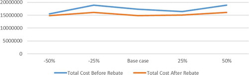
Sensitivity analysis is performed to study the impact the model parameters toward the quality improvement level at suppliers side and objective function. Those model parameters that we investigate for their impact on both quality improvement level and objective function are appraisal cost, failure cost, and prevention cost. Those model parameters are changed by 25% and 50% higher and lower from the base case. We first investigate how the failure cost influence the model’s behavior. Figure 2 shows the impact of the change of failure cost to total suppliers cost. There are no specific pattern of the total suppliers cost due to decreasing or increasing the failure cost. But if we compare the quality level both before and after rebates of all suppliers, then higher failure cost will increase the quality levels. This behavior reveals that higher failure cost will prevent the system to produce high defect products. The differences between total suppliers cost before and after rebates range from 9.5% to 14.6% which considered as significant.

Figure 2. The impact of appraisal cost to total suppliers cost.

We further analyse the impact of appraisal cost to the suppliers quality improvement level and suppliers total cost. Figure 3 shows the impact of appraisal cost to suppliers total cost. The figure shows higher appraisal cost will lowering the suppliers total cost. This results show that higher appraisal cost will increase the quality level of component produced by the suppliers. The differences between total suppliers cost before and after rebates range from 3.8% to 14.9% which considered as significant.

Figure 3. The impact of appraisal cost to total supplier cost.

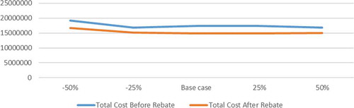
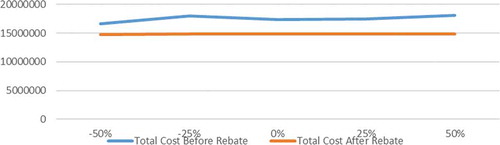
Figure 4 shows the impact of prevention cost to total suppliers cost. The figure shows that there are relatively no changes in total suppliers cost after rebate. There are also relatively no changes in suppliers quality level. This behavior shows that prevention cost relatively has no significant effects on quality level and its improvement. The differences between total suppliers cost before and after rebates range from 11.4% to e17.9% which considered as significant. From all quality cost, the prevention cost gives the most significant difference in suppliers total cost before and after rebate.

Figure 4. The impact of prevention cost to total suppliers cost.

4. Conclusions

In this paper, we proposed an optimization model to determine the optimum allocation of component to improve the quality level of suppliers and minimizing the total cost comprises of manufacturing cost, quality loss, and lateness cost. Rebate is used to increase the effort of supplier to improve the quality of components. The manufacturer will receive components with higher quality after rebate. From the optimization results, the quality level of components after rebate is higher than the quality level of component before rebate. Hence, the quality loss of supplier is reduced after rebate. We found from sensitivity analysis that the failure cost, appraisal cost, and prevention cost have significant impacts on the total suppliers cost. Among those costs prevention cost gives the most significant effect on total suppliers cost. For future research, the model can be extended by involving learning investments and analyse the effects of forgetting or remanufacturing decisions to the system.

Cover Image

Source: Author

Additional information

Funding

The authors received no direct funding for this research.

Notes on contributors

Cucuk Nur Rosyidi

Cucuk Nur Rosyidi is a Professor in Industrial Engineering Department at Universitas Sebelas Maret Surakarta. His research interests include make or buy decision modeling, product design and development, and quality engineering. He currently serves as the head of a research group, namely Center of Research in Manufacturing Systems (CRiMS) which focuses on several issues in design and production optimization including inventory.

Namrotul Uela Fatakunul Imamah

Namrotul Uela Fatakunul Imamah is an alumni of Industrial Engineering Department at Universitas Sebelas Maret Surakarta. She finished the undergraduate program in 2017 and currenly works at a big manufacturing company in Jakarta, Indonesia. Her research interest is mainly in the field of production system.

Wakhid Ahmad Jauhari

Wakhid Ahmad Jauhari is a lecturer in Industrial Engineering Department at Universitas Sebelas Maret Surakarta. His master degree was obtained from Institut Teknologi Sepuluh Nopember Surabaya, Indonesia in the field of Supply Chain Management. His research interests are in the fields of supply chain and inventory control, mathematical modeling, and optimization.

References

- Angkiriwang, R., Pujawan, I. N., & Santosa, B. (2014). Managing uncertainty through supply chain flexibility: Reactive vs. proactive approach. Production and Manufacturing Research, 2(1), 50–22. https://doi.org/10.1080/21693277.2014.882804
- Banaeian, N., Mobli, H., Nielsen, I. E., & Omid, M. (2015). Criteria definition and approaches in green supplier selection – A case study for raw material and packaging of food industry. Production and Manufacturing Research, 3(1), 149–168. https://doi.org/10.1080/21693277.2015.1016632
- Bardhan, I., Whitaker, J., & Mithas, S. (2006). Information technology, production process outsourcing, and manufacturing plant performance. Journal of Management Information Systems, 23(2), 13–40. https://doi.org/10.2753/MIS0742-1222230202
- Cao, Y., Mao, J., Ching, H., & Yang, J. (2009). A robust tolerance optimization method based on fuzzy quality loss. Institution of Mechanincal Engineers, Part C: Journal of Mechanical Engineering Science, 223(11), 2647–2653. SAGE Publishing. https://doi.org/10.1243/09544062JMES1451
- Chase, K. W., Loosli, B. G., Greenwood, W. H., & Hauglund, L. F. (1990). Least cost tolerance allocation for mechanical assemblies with automated process selection. Manufacturing Review, 3(1), 49–59. http://adcats.et.byu.edu/Publication/89-4/Proc_Sel_Paper1.PDF
- Ding, Y., Ceglarek, D., Jin, J., & Shi, J. (2000). Process-oriented tolerances synthesis for multistage manufacturing system. American Society of Mechaninal Engineers, Manufacturing Engineering Division, MED, 11, 15–22.
- Duarte, B. P., Oliveira, N. M., & Santos, L. O. (2016). Dynamics of quality improvement programs - optimal investment policies. International Journal of Computers and Industrial Engineering, 91, 215–228. https://doi.org/10.1016/j.cie.2015.11.020
- Group, P. R. (2016). Outsourcing manufacturing: A 20/20 view. E2Open and Supply Chain Management Review.
- Hallgren, M., & Olhager, J. (2006). Differentiating manufacturing focus. International Journal of Production Research, 44(18–19), 3863–3878. https://doi.org/10.1080/00207540600702290
- Harrington, H. J. (1987). Poor quality cost. ASQC New York Press.
- Kusukawa, E., Kudo, K., & Ohta, H. (2006). Rebate system for quality improvement under supply chain environment. International of Federation Automatic Control Proceedings Volumes, 12(1), 617–622. https://doi.org/10.3182/20060517-3-FR-2903.00315
- Maia, L. C. C., Fonseca, E. R., de Castro, M., & Carrijo, M. C. (2015). The production outsourcing in emerging countries: The analysis of the opportunities under the theory of costs economy. Proceedings of 26 th production and operation management annual conference, Washington, DC, USA
- Montgomery, D. C. (2001). Introduction to statistical quality control. John Wily&Sons.
- Mustajib, M. I., & Irianto, D. (2010). An integrated model for process selection and quality improvement in multi-stage processes. Journal of Advanced Manufacturing Systems, 9(1), 31–48. https://doi.org/10.1142/S0219686710001788
- Oncu, A. A., Oner, M. A., & Basoglu, N. (2003). Make or Buy analysis for local manufacture or import decisions in defense system procurments using AHP: The case of Turkey. Portland international conference on management of engineering and technology, Portland, USA
- Oracle Corporation. (2008). One-minute spotlight optquest: finding the best solutions under uncertain conditions.Oracle Corporation.
- Porter, M. (1980). Competitive Strategy. Free Press.
- Pratama, M. A., Rosyidi, C. N., & Pujiyanto, E. (2018). Two stages optimization model on make or buy analysis and quality improvement considering learning and forgetting curve. Journal of Industrial Engineering and Management, 11(4), 794–813. https://doi.org/10.3926/jiem.2615
- Rosyidi, C. N., Akbar, R. R., & Jauhari, W. A. (2014). Make or buy analysis model based on tolerance design to minimize manufacturing cost and quality loss. Makara Journal of Technology, 18(2), 86–90. https://doi.org/10.7454/mst.v18i2.400
- Rosyidi, C. N., Fatmawati, A., & Jauhari, W. A. (2016a). An integrated optimization model for product design and production allocation in a make to order manufacturing system. International Journal of Technology, 7(5), 819–830. https://doi.org/10.14716/ijtech.v7i5.1173
- Rosyidi, C. N., Nugroho, A. W., Jauhari, W. A., Suhardi, B., & Hamada, K. (2016c). Quality improvement by variance reduction of component using learning investment allocation model. International conference on industrial engineering and engineering management, IEEM 2016, Bali, Indonesia (pp. 391–394). https://doi.org/10.1109/IEEM.2016.7797903.
- Rosyidi, C. N., Pamungkas, I. P. B., Jauhari, W. A., Suhardi, B., & Hamada, K. (2016d). An investment allocation model for quality improvement to reduce component variances at manufacturer and supplier side to maximize the return on investment.International conference on industrial engineering and engineering management, IEEM 2016, Bali, Indonesia (pp. 1713–1716). https://doi.org/10.1109/IEEM.2016.7798170
- Rosyidi, C. N., & Pratama, M. A. (2018). Two-stage optimization model for process/supplier selection, component allocation, and quality improvement. Cogent Engineering, 5(1), 1–16. https://doi.org/10.1080/23311916.2018.1557504
- Rosyidi, C. N., Pratama, M. A., Jauhari, W. A., Hamada, K., & Suhardi, B. (2016b). Make or buy analysis model in a multi-stage manufacturing process. International conference on industrial engineering and engineering management, IEEM 2016, Bali, Indonesia. https://doi.org/10.1109/IEEM.2016.7798022
- Sofiana, A., Rosyidi, C. N., & Pujiyanto, E. (2019). Product quality improvement model considering quality investment in rework policies and supply chain profit sharing. Journal of Industrial Engineering International, 15(4), 637–649. https://doi.org/10.1007/s40092-019-0309-7
- Sousa, R., & Voss, C. A. (2007). Operational implications of manufacturing outsourcing for subcontractor plants: An empirical investigation. International Journal of Operations & Production Management, 27(9), 974–997. https://doi.org/10.1108/01443570710775829
- Subramanian, N., Abdulrahman, M. D., & Rahman, S. (2014). Sourcing complexity factors on contractual relationship: Chinese suppliers’ perspective. Production & Manufacturing Research, 2(1), 558–585. https://doi.org/10.1080/21693277.2014.949361
- Teeravaraprug, J. (2008). Outsourcing and vendor selection model based on taguchi loss function. Songklanakarin Journal of Science and Technology, 30(4), 523–530. https://rdo.psu.ac.th/sjstweb/journal/30-4/0125-3395-30-4-523-530.pdf
- Veldman, J., & Gaalman, G. (2014). A model of strategic product quality and process improvement incentives. International Journal of Production Economics, 149, 202–210. https://doi.org/10.1016/j.ijpe.2013.03.002
- Zhang, G. (1996). Simultaneous tolerancing for design and manufacturing. International Journal of Production Research, 34(12), 3361–3382. https://doi.org/10.1080/00207549608905095