Derivation of closed-form expression for optimal base stock level considering partial backorder, deterministic demand, and stochastic supply disruption

Abstract

In the presence of stochastic supply disruption, the optimal variables of an inventory policy must be determined appropriately. Considering a two-echelon system comprised of a supplier and a retailer, the objective of this research is to help the retailer derives the optimal base stock level that achieves the minimum costs per unit of time regarding the stochastic unavailability of the supplier. The expression of the optimal base stock level is determined in closed-form in consideration of a continuous random variable of a disruption length together with a partial backorder of shortage inventory. A solution method which facilitates the retailer to derive the correct expression for the optimal base stock level is proposed. The applicability of the proposed solution method is illustrated through numerical experiments.

Keywords:

• supply disruption
• periodic review base stock policy
• closed-form expression
• optimal base stock level
• partial backorder

PUBLIC INTEREST STATEMENT

Considering the effect of supply disruption to derive an optimal inventory policy is essential in order for a firm to achieve the minimum costs per unit of time. In this research work, a solution method that helps derive the optimal variable of an inventory policy is proposed. For the sake of reality, the proposed solution method is based on the premise that the disruption length is an independent variable, and the shortage inventory can be either lost sale, full backorder, or partial backorder. Implementing the proposed method, it requires a few steps; therefore, a manager conveniently derives the optimal inventory policy in the presence of stochastic supply disruption.

1. Introduction

Adopting an outsourcing strategy, a firm gains competitive advantage from focussing only on a few business core competencies that substantially enhances the firm’s performance (Prahalad & Hamel, 1990). This strategy allows the firm not only to increase the return on investment but also to concentrate more on the marketing and sale functions to leverage the firm’s buying power (De Kok & Graves, 2003). Nevertheless, the letting of suppliers to supply goods instead of manufacturing products in-house inevitably exposes the firm to uncertain supply problems. There are various types of uncertain supply problems that a firm could face, such as quality of supply batch, limited capacity of supply, yield, and supply disruption.

Supply disruption causes the firm to experience a shortage of input materials, stock out, loss of goodwill, and increased costs, as a result of the temporary unavailability of supply sources. There are various causes of the supply disruption problem, including labor strike at a supplier’s facility (Parlar & Perry, 1996), fire at a sub-supplier’s facility (Norrman & Jansson, 2004), supplier’s production problem (Greising & Johnsson, 2007). Considering some practical examples of the effect of supply disruption, Ericsson encountered a shortage of electronic chips from a supplier who ran into some trouble, and the loss was 400 USD million due to inability to respond to key customer demand during a peak selling season (Norrman & Jansson, 2004). The delivery delay for a newly launched product, the Boeing 787 Dreamliner, cut off cash flow by 2.5 USD billion due to a screw supply shortage problem (Greising & Johnsson, 2007). Therefore, in the presence of stochastic supply disruption, some strategies must be employed properly, and Tomlin (2006) proposed a list of strategies as well as discussing the situations where the appropriate strategies could be employed. Focussing on inventory holding strategy, its concept is to hold extra inventory to increase responsiveness during a supply disruption period.

This research work considers a two-echelon system comprising a supplier, who randomly runs into problems leading to unavailability to respond to orders temporarily, and a retailer, who has to devise an inventory policy to manage the supply disruption problem. Neither order too much nor too few is good for the retailer. The question regarding the optimal inventory policy, therefore, arises. The retailer applies a periodic review base stock policy. Ordinarily, at a review point in time, the retailer places an order, and the receipt is immediate. However, faced with the supplier’s troubles, the retailer must wait until the supplier resolves the troubles before placing an order. The time elapsed from the occurrence of a disruption to the end of the disruption refers to the disruption length. There are two cases of disruption length found in the existing literature, i.e., a multiple of inventory review intervals, and continuous length. Considering the continuous length of supply disruption gains advantage in that it not only helps derive a more precise optimal level of base stock but also presents the reality (Saithong & Luong, 2019). Thus, we consider it in this study. Unmet demand from on-hand inventory is partially back-ordered, and the rest is lost sale. The component of total costs comprises time-dependent holding costs (monetary unit per unit and per unit of time), backorder costs (monetary unit per unit and per unit of time), and lost sale costs (monetary unit per unit). The objective of this study is to derive the optimal base stock level for the retailer, which helps achieve the minimum costs per unit of time.

Taking into consideration the continuous variable of supply disruption length together with the partial backorder of shortage inventory to derive the optimal variable in a closed-form expression leads to practical situations that facilitate managers to derive the optimal level of base stock precisely. Even though some of the existing literature deals with such a problem, a few studies considered the continuous variable of supply disruption length. Since treating the disruption length as an independent continuous random variable could be more realistic and could help derive an accurate optimal level of base stock, we should include this feature in the model. Even if Hsieh and Putera (2018) and Saithong and Luong (2019) considered the continuous variable of supply disruption length, they did not consider the partial backorder, and the optimal inventory policy variable cannot be derived in a closed-form expression. Another important feature is the way to handle the shortage inventory of the retailer. Three possible cases may happen, i.e., lost sale, partial backorder, and full backorder. Although De and Mahata (2020) and Taleizadeh and Dehkordi (2017) considered the partial backorder and the optimal inventory policy variables can be derived in a closed-form expression, they did not consider the continuous length of supply disruption. To the best of our knowledge, none of the existing literature derives the closed-form expression for the optimal base stock level under a periodic review base stock inventory system by taking into consideration the continuous variable of disruption length together with the partial backorder of shortage inventory. Therefore, this study aims to fulfill this research gap.

The remaining sections of this paper are organized as follows. The existing literature related to the derivation of optimal inventory policy will be reviewed. Next, the problem definition will be addressed, and we will formulate the problem analytically. After that, numerical experiments will be conducted. Lastly, we will draw conclusions as well as provides directions for further research.

2. Literature review

Parlar and Berkin (1991) were one of the first to investigate the supply disruption effect on a traditional EOQ model. The mathematical model developed by Parlar and Berkin (1991) was revised by Berk and Arreola‐Risa (1994). Parlar et al. (1995) considered a periodic review inventory policy with backlogging under both stochastic supply disruption effect and stochastic demand. The supply process follows a geometric distribution so that inventory can only be either replenished or unfulfilled. Parlar and Perry (1996) studied the effect of having multiple supply sources where each supply source randomly runs into problems so that it cannot respond to an order. The result reveals that the optimal inventory policy approaches an EOQ model as the number of sources of supply becomes larger. Mohebbi (2003) investigated the stochastic supply disruption effect on a continuous review inventory system. It was assumed that the demand follows a compound Poisson distribution, and the lead time follows an Erlang distribution. The exact analytical expression of the costs is presented, and numerical experiments are conducted in order to derive the optimal inventory policy variables. Relaxing the assumption of an Erlang distributed lead time of Mohebbi (2003), Mohebbi (2004) considered Hyperexponentially distributed lead time. Atasoy et al. (2012) examined the value of information when the information about supply availability can be provided by the supplier in advance. The value of the information depends on the degree of stationary of supply availability; that is, the value of the information increases with the degree of supply variability. Schmitt and Snyder (2012) considered both disruption and yield uncertainty to derive the optimal base stock level. Lewis et al. (2013) dealt with temporary closure in a port-of-entry problem by using an inventory holding strategy and examined the effect of the temporary closure on supply chain costs. Ciarallo and Niranjan (2014) took a capacity-constrained problem characterized as the all-or-nothing type into consideration for deriving the optimal order-up-to level. Firouzi et al. (2014) considered an (s,S) periodic review inventory system under stochastic supply disruption for two products. The proposed model helps determine the optimal production quantity, where there are switching costs between these two products. Hsieh and Putera (2018) examined the manufacturer’s decision sourcing from an unreliable supplier. Both optimal order quantity and optimal restoration capacity, which helps minimize total costs, are derived through numerical experiments. Sevgen and Sargut (2019) examined the importance of the non-zero re-order point in a continuous review system when both supplier and retailer are subject to stochastic disruption. The results reveal cost savings from the non-zero re-order policy in certain cases. Saithong and Luong (2019) investigated the supply disruption effect on a periodic review base stock inventory system. They considered the supply disruption length as a continuous random variable, and the optimal policy variable can always be derived. Furthermore, the numerical results confirm the importance of taking into consideration the continuous stochastic variable of disruption length. Saithong and Luong (in press) considered an (r,S) continuous review inventory policy. The function of the expected cost per unit of time is analytically formulated, and the existence of optimal policy variables are confirmed through numerical experiments. It should be noted that none of the above papers derives the optimal inventory policy variables in a closed-form expression.

Of the existing literature that derives the optimal variables in a closed-form expression, Güllü et al. (1999) considered three possible supply states in the derivation of optimal order-up-to level, namely, fully available, fully unavailable, and incompletely available. A simple newsboy-like formula is proposed in order to derive the optimal variables of the inventory policy in the case of all-or-nothing supply states. Li et al. (2004) investigated the case demand depends on the state of the supplier, and the supply status is formulated by using an alternating renewal process. Warsing et al. (2013) derived the optimal base stock level in a closed-form expression for some distributions of demand. Konstantaras et al. (2019) derived a closed-form expression for optimal variables in an (S,T) periodic review system. Both continuous and end-of-period cost accounting schemes are considered.

Due to the merits of closed-form expression, some of the existing literature put effort into the approximation of the optimal inventory policy variables. Heimann and Waage (2007) provided closed-form approximate expressions for optimal variables of a (Q,r) continuous review system in the case where the supplier randomly runs into disruption. Qi et al. (2009) studied the case where both the supplier and retailer are subject to disruption and proposed a closed-form approximate formula for the optimal order quantity as well as the error bounds. Schmitt et al. (2010) developed a closed-form approximation for the optimal base stock level. Snyder (2014) introduced an effective approximation of the EOQ model in which the theoretical and numerical bounds on error in the cost are proposed. Bakal et al. (2017) investigated the value of allowing disruption order, which is placed right at the beginning of the disruption period. Allowing the disruption order, the cost significantly reduces. Furthermore, a simple heuristic is proposed, which helps determine the optimal disruption order.

Some existing literature considers supply disruption as a result of the rejection of a defective supply batch. Skouri et al. (2014) derived an exact expression for the optimal order quantity when the supply batch was considered defective and was rejected on arrival. The shortage inventory was fully backordered. Later, Salehi et al. (2016) relaxed the assumption of the full backorder of shortage inventory and considered the case of a partial backorder and proposed a solution method. Taleizadeh and Dehkordi (2017) considered the sampling inspection policy in addition to partial backorder and a possibly defective supply batch. Subsequently, relaxing the assumption of full payment at the time of the retailer’s receipt, Taleizadeh (2017) considered the case of advance payment, proposing a solution algorithm and conducting numerical examples as well as sensitivity analyses. De and Mahata (2020) considered various cost components as a linguistic triangular dense fuzzy lock set in order to determine the optimal length of the consecutive supply batch and the optimal time fraction of positive inventory level in an inventory cycle.

Of the recent literature considering various types of uncertainty to acquire the optimal inventory policy, Jauhari et al. (2017) investigated into a production-inventory system considering imperfect production, partial backorder, and inspection error to optimize the vendor’s production rate, buyer’s review period length, and the number of deliveries. Relaxing the assumptions of fixed ordering cost and vendor’s fixed set up cost, Jauhari and Saga (2017) considered fuzzy ordering cost and reducible setup cost. Besides, considering the impact of carbon incentive and penalty policy, Saga et al. (2019) determined the optimal inventory decisions under the constrained service level. Fathalizadeh et al. (2019) considered the effect of product deterioration and the stochastic inflation rate to determine the optimal inventory policy. A comparison between the average annual cost modeling method and the discounted costs modeling method was made. Zhang et al. (2019) studied a system comprised of a manufacturer, a backup manufacturer, and multiple distributors. The distributors could receive goods from the backup manufacturer and/or other distributor, and a robust emergency strategy was designed to tackle the supply disruption problem. Lücker et al. (2019) tackled the supply disruption problem by using inventory and reserve capacity. The optimal inventory levels and the reserve capacity production rate were derived.

For other interesting literature, Shahbaz et al. (2019) addressed the effect of the disruption problem on public sector construction projects. The disruption problem caused cost overruns and delays. Flexibility and collaboration with stakeholders were the approaches used to tackle the problem. Orgeldinger (2018) presented different approaches to mitigate the market risks in banks’ trading systems based on a specified standard. The new implementation could not only mitigate risks but also reduce operational implementation burdens. Spilbergs (2020) investigated the risk drivers of housing loans in the presence of a financial crisis. It was found that various drivers could have an effect on total risks: unemployment, income, GDP, house price index, wage growth, credit history, etc.

Focusing on a periodic review base stock policy, to the extent of our knowledge, none of the existing literature derives the optimal variable in a closed-form expression based simultaneously on a continuous variable of the disruption length and partial backorder of shortage inventory. Table 1 shows the comparison between the existing literature and this research work. Even though Hsieh and Putera (2018) and Saithong and Luong (2019) considered the continuous variable of the disruption length, however, the shortage inventory was fully back-ordered, and the issue of a closed-form expression for the optimal variable was not of interest. Even though Salehi et al. (2016), Taleizadeh and Dehkordi (2017), Taleizadeh (2017), and De and Mahata (2020) considered the partial backorder of shortage inventory and derived the optimal variables of an inventory policy in closed-form expressions, however, the disruption length is a multiple of the review intervals. The closed-form expression gain benefits, as discussed in Heimann and Waage (2007), Qi et al. (2009), Schmitt et al. (2010), and Snyder (2014), and the importance of considering the disruption length as an independent variable from the inventory review interval is discussed in Saithong and Luong (2019). In summary, this research work contributes to the literature by taking the continuous variable of the supply disruption length together with the partial backorder of shortage inventory into consideration for deriving the optimal base stock level in a closed-form expression.

Table 1. The comparison between the existing literature and the present research work

Authors	Continuous variable of supply disruption length	Partial backorder	Exact closed-form expressions for optimal variables
Parlar et al. (1995)
Güllü et al. (1999)			●
Li et al. (2004)			●
Schmitt et al. (2010)
Atasoy et al. (2012)
Schmitt and Snyder (2012)			●
Lewis et al. (2013)			●
Warsing et al. (2013)			●
Ciarallo and Niranjan (2014)
Firouzi et al. (2014)
Skouri et al. (2014)			●
Salehi et al. (2016)		●	●
Taleizadeh (2017)		●	●
Taleizadeh and Dehkordi (2017)		●	●
Hsieh and Putera (2018)	●
Konstantaras et al. (2019)			●
Saithong and Luong (2019)	●
De and Mahata (2020)		●	●
This research work	●	●	●

3. Problem description and mathematical model formulation

Taking the two-echelon system into consideration, the supplier randomly runs into problems, and the retailer has to devise an inventory policy to help mitigate the effect of stochastic supply disruption. The retailer operates under a periodic review base stock policy in which the retailer inspects the inventory position at every fixed interval (the review interval) and places an order so that the inventory position is brought up-to the level of base stock. After placing the order, the receipt will be immediate if the supplier is available. Nevertheless, if the supply is disrupted at the retailer’s inventory review point in time, the retailer is not allowed to place an order and is obligated to wait until the supplier turns to be available. The duration the retailer waits for placing the order is random and does not depend on the inventory review interval. Unmet demand from inventory is partially back-ordered and the rest is lost sale. The retailer’s interest is to determine the optimal base stock level which helps minimize the costs per unit of time.

According to the above problem description, the following are assumed.

• The demand per day is a constant, i.e., demand is deterministic.

• The stochastic supply disruption profile is considered, i.e., the disruption length and disruption arrival are exponentially distributed.

• Only effective supply disruption is considered; that is, it always delays the retailer’s order once it occurs.

Then, the list of notations used in this research is as shown in Table 2.

Table 2. List of notations

Notation	Description
$\lambda$	The arrival rate of supply disruption
$\mu$	Parameter of exponential distribution representing the length of a supply disruption
$\beta$	The fraction of amount of demand that is back-ordered
$D$	Demand per day
$C_H$	Inventory holding costs per unit per day
$C_S$	Costs of lost sale per unit
$C_B$	Costs of backorder per unit per day
$X$	The random variable representing the time until an arrival of supply disruption which is assumed to follow an exponential distribution with rate $\lambda$, i.e., the density function of X is $f_X(x)=\lambda e^{-\lambda x}$
$Y$	The random variable representing the length of a supply disruption which is assumed to follow an exponential distribution with rate$\mu$, i.e., the density function of Y is$f_Y(y)=\mu e^{-\mu y}$
$N$	The random variable representing the number of inventory cycles in a renewal cycle
$T$	Length of an inventory review period
${\left.A\right|}_{A>T}$	The random variable representing the length of the last inventory cycle in a renewal cycle
$Z$	The random variable representing the length of a renewal cycle
$W$	The random variable representing the time elapsed from the last order placing before a disruption occurs until the arrival of the disruption
$S$	Base stock level
$i$	Indices of possible scenarios of a renewal cycle: $i=1$: The case when inventory is shortage in non-disrupted cycles $i=2$: The case when inventory is not shortage in non-disrupted cycles
$TC{U}^{\left\{i\right\}}\left(S\right)$	Total costs per day, as a function of $S$, for case $i$
$ND{C}^{\left\{i\right\}}$	Total costs in a non-disrupted cycle for case $i$
$D{C}^{\left\{i\right\}}$	Total costs in the disrupted cycle, i.e., the last inventory cycle, for case $i$
$S^{\ast \left\{i\right\}}$	Optimal base stock level for case $i$
$S^{\ast }$	Optimal base stock level
$TCU\left(S^{\ast }\right)$	The minimum cost per time unit

Because the retailer’s interest is to minimize the total costs per day, the renewal reward theorem is used to formulate the retailer’s expected cost per day function (Ross, 1996). The length of a renewal cycle is the interval between the occurrences of two consecutive disruptions, as seen in Figure 1. A renewal cycle contains both inventory cycles in which disruption does not take place (non-disrupted inventory cycles) and an inventory cycle in which supply disruption takes place. The length of an inventory cycle is measured from the two consecutive receipts (receipt-to-receipt). For non-disrupted inventory cycles, the inventory cycle length is the same as the inventory review interval. On the other hand, the length of the last inventory cycle is perhaps longer than the inventory review interval due to the unavailability of supply ceasing the retailer’s order. The illustration of the possible scenarios of a renewal cycle is depicted in Figure 1.

Figure 1. Possible cases of renewal cycle in the presence of supply disruption.

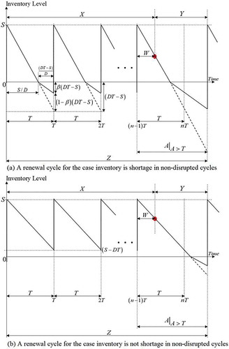
There are two possible scenarios for a renewal cycle in the presence of supply disruption, as seen in Figure 1(a and b). It should be noted that where shortage inventory is fully backordered and supply disruption does not exist (supply is always available), there will be a planned backorder for each inventory cycle, and the formula that helps derive the optimal base stock level appears in general text-books, such as Axsäter (2015). In the presence of stochastic supply disruption, the optimal base stock level is supposed to be higher than this level. Therefore, the stochastic supply disruption will raise the optimal base stock level and causes either of the cases. We will derive the closed-form expression of the optimal base stock level for each case and provide a solution method in order to identify the right scenario of a renewal cycle so that we can derive the correct expression of the optimal base stock level.

The remaining parts of this section are organized as follows. The derivation of the optimal base stock level in the presence of stochastic supply disruption is shown in subsection 3.1. For more detail, in this subsection, the expected cost functions and the corresponding components are analyzed regarding the possible scenarios of a renewal cycle. Then, in subsection 3.2, a solution method that helps derive the correct expression for the optimal base stock level is proposed.

3.1. Optimal base stock level in the presence of stochastic supply disruption

As introduced earlier, there are two possible cases of a renewal cycle, and we need to formulate the expected costs per day function for these two cases separately. In this section, we discuss these two cases, and the optimal base stock level for each case is addressed.

3.1.1. Optimal base stock level for the case inventory is shortage in non-disrupted cycles

Before deriving the optimal base stock level, which helps minimize the total costs per day for this case, we first need to formulate the function of expected costs per day. The total costs in a renewal cycle include holding costs, backorder costs, and lost sale costs. In a renewal cycle, there are $\left(E\left[N\right]-1\right)$ cycles in which supply disruption is not effective and a cycle in which supply disruption is effective. Therefore, the expected costs for the case of ineffective supply disruption is $E\left[ND{C}^{\left\{1\right\}}\right]\left(E\left[N\right]-1\right)$, and for the case of effective supply disruption, the expected costs is $E\left[D{C}^{\left\{1\right\}}\right]$. Regarding the cycle length, the expected cycle length for the case of effective disruption and ineffective disruption are $E\left[{\left.A\right|}_{A>T}\right]$ and $T$, respectively. Incorporating these two cases and dividing by the expected renewal cycle length, the expected total costs per day can be derived as:

(1) $E\left[TC{U}^{\left\{1\right\}}\left(S\right)\right]=\frac{E\left[ND{C}^{\left\{1\right\}}\right]\left(E\left[N\right]-1\right)+E\left[D{C}^{\left\{1\right\}}\right]}{E\left[Z\right]}=\frac{E\left[ND{C}^{\left\{1\right\}}\right]\left(E\left[N\right]-1\right)+E\left[D{C}^{\left\{1\right\}}\right]}{T\left(E\left[N\right]-1\right)+E\left[{\left.A\right|}_{A>T}\right]}$(1)

In order to derive $E\left[TC{U}^{\left\{1\right\}}\left(S\right)\right]$, we need to determine $E\left[N\right]$, $E\left[{\left.A\right|}_{A>T}\right]$, $E\left[ND{C}^{\left\{1\right\}}\right]$, and $E\left[D{C}^{\left\{1\right\}}\right]$ accordingly. We will determine these components in the following subsections.

3.1.1.1. Determination of $E\left[N\right]$

Referring to Saithong and Luong (2019), the random variable $N$ has a relationship with the random variable $X$. By definition, $E\left[N\right]=\sum _{n=1}^{\mathrm{\infty }}nP\left\{N=n\right\}$ and $P\left\{N=n\right\}=P\left\{\left(n-1\right)T\le X\le nT\right\}$. $E\left[N\right]$ can be expressed as

(2) $E\left[N\right]=\frac{1}{1-e^{-\lambda T}}$(2)

3.1.1.2. Determination of $f_{{\left.A\right|}_{A>T}}(a)$ and $E\left[{\left.A\right|}_{A>T}\right]$

From Figure 1, it can be seen that the random variable ${\left.A\right|}_{A>T}$ has a relationship with both the random variable $W$ and the random variable $Y$, namely, ${\left.A\right|}_{A>T}=W+Y$. The probability density function of ${\left.A\right|}_{A>T}$ can be determined from the convolution of $W$ and $Y$. The derivation of $f_{{\left.A\right|}_{A>T}}(a)$ is shown in Saithong and Luong (2019). Then, by definition, $E\left[{\left.A\right|}_{A>T}\right]={\int }_T^{\mathrm{\infty }}a{f}_{{\left.A\right|}_{A>T}}(a)da$. Referring to Saithong and Luong (2019), the expressions of $f_{{\left.A\right|}_{A>T}}(a)$ and $E\left[{\left.A\right|}_{A>T}\right]$ follow:

(3) $f_{{\left.A\right|}_{A>T}}(a)=\mu e^{-\mu \left(a-T\right)};a>T$(3)

(4) $E\left[{\left.A\right|}_{A>T}\right]=T+\frac{1}{\mu }$(4)

3.1.1.3. Determination of $E\left[ND{C}^{\left\{1\right\}}\right]$

For the total costs in a non-disrupted cycle, it consists of inventory holding costs, backorder costs, and lost sale costs. The inventory holding costs is $C_H\left(\frac{S}{2}\right)\left(\frac{S}{D}\right)$. The costs of backorder is $C_B\left(\frac{\beta \left(DT-S\right)}{2}\right)\left(\frac{DT-S}{D}\right)$. The costs of lost sale is $C_S\left(1-\beta \right)\left(DT-S\right)$. Therefore, $E\left[ND{C}^{\left\{1\right\}}\right]$ can be derived as:

(5) $E\left[ND{C}^{\left\{1\right\}}\right]=\frac{C_H{S}^2}{2D}+\frac{C_B\beta {\left(DT-S\right)}^2}{2D}+C_S\left(1-\beta \right)\left(DT-S\right)$(5)

3.1.1.4. Determination of $E\left[D{C}^{\left\{1\right\}}\right]$

In order to derive $E\left[D{C}^{\left\{1\right\}}\right]$, we need to determine $E\left[{\left.D{C}^{\left\{1\right\}}\right|}_{\left.A\right|A>T=a}\right]$ first. Utilizing the computing of the expectation by conditioning technique, we will get $E\left[D{C}^{\left\{1\right\}}\right]=\underset{T}{\overset{\mathrm{\infty }}{\int }}E\left[{\left.D{C}^{\left\{1\right\}}\right|}_{\left.A\right|A>T=a}\right]f_{{\left.A\right|}_{A>T}}(a)da$. From Figure 2, evaluating at ${\left.A\right|}_{A>T}=a$, the expected holding costs, backorder costs, and lost sale costs are $C_H\left(\frac{S}{2}\right)\left(\frac{S}{D}\right)$, $C_B\left(\frac{\beta \left(Da-S\right)}{2}\right)\left(\frac{Da-S}{D}\right)$, and $C_S\left(1-\beta \right)\left(Da-S\right)$, respectively. Then, $E\left[{\left.D{C}^{\left\{1\right\}}\right|}_{\left.A\right|A>T=a}\right]$ can be derived as:

$E\left[{\left.D{C}^{\left\{1\right\}}\right|}_{\left.A\right|A>T=a}\right]=\frac{C_H{S}^2}{2D}+\frac{C_B\beta {\left(Da-S\right)}^2}{2D}+C_S\left(1-\beta \right)\left(Da-S\right)$

Figure 2. The last inventory cycle when $i=1$.

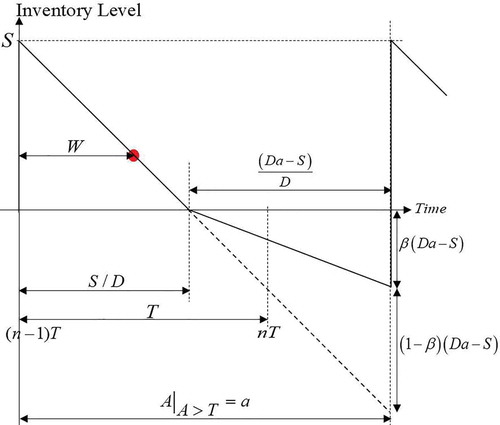
The first term of the above equation represents the expected holding costs, which can be determined from the $C_H$ value multiplies by the area under the inventory level curve when inventory is holding in Figure 2. The second term represents the expected backorder costs. It can be determined from the $C_B$ value multiplies by the area under the inventory level curve when the inventory is shortage, but back-ordered in Figure 2. The last term represents the costs of lost sale of shortage inventory. The lost sale costs can be determined from the $C_S$ value multiplies by the number of units of lost sale. After that, $E\left[D{C}^{\left\{1\right\}}\right]$ can be derived as:

$E\left[D{C}^{\left\{1\right\}}\right]=\underset{T}{\overset{\mathrm{\infty }}{\int }}\left(\frac{C_H{S}^2}{2D}+\frac{C_B\beta {\left(Da-S\right)}^2}{2D}+C_S\left(1-\beta \right)\left(Da-S\right)\right)f_{{\left.A\right|}_{A>T}}(a)da$

From (3), $f_{{\left.A\right|}_{A>T}}(a)=\mu e^{-\mu \left(a-T\right)}$ and the above equation yields:

$\begin{array}{rl}& E\left[D{C}^{\left\{1\right\}}\right]=\underset{T}{\overset{\mathrm{\infty }}{\int }}\left(\frac{C_H{S}^2}{2D}\right)\left(\mu e^{-\mu \left(a-T\right)}\right)da+\underset{T}{\overset{\mathrm{\infty }}{\int }}\left(\frac{C_B\beta {\left(Da-S\right)}^2}{2D}\right)\left(\mu e^{-\mu \left(a-T\right)}\right)da\\ & +\underset{T}{\overset{\mathrm{\infty }}{\int }}{C}_S\left(1-\beta \right)\left(Da-S\right)\left(\mu e^{-\mu \left(a-T\right)}\right)da\end{array}$

Finally, we have:

(6) $E\left[D{C}^{\left\{1\right\}}\right]=\frac{C_H{S}^2}{2D}+C_B\beta \left(\frac{D{T}^2}{2}+\frac{S^2}{2D}+\left(T+\frac{1}{\mu }\right)\left(\frac{D}{\mu }-S\right)\right)+C_S\left(1-\beta \right)\left(D\left(T+\frac{1}{\mu }\right)-S\right)$(6)

3.1.1.5. Optimal base stock level for the case$i=1$

The optimal base stock level, which helps achieve the minimum$E\left[TC{U}^{\left\{1\right\}}\left(S\right)\right]$, can be derived from $\frac{dE\left[TC{U}^{\left\{1\right\}}\left(S\right)\right]}{dS}=0$. Therefore, we need to know the exact expression of $E\left[TC{U}^{\left\{1\right\}}\left(S\right)\right]$ first and, by replacing all corresponding components in (1) with $E\left[N\right]$, $E\left[ND{C}^{\left\{1\right\}}\right]$, $E\left[{\left.A\right|}_{A>T}\right]$, $E\left[D{C}^{\left\{1\right\}}\right]$ derived in (2), (5), (4), and (6), respectively, we will have:

(7) $E\left[TC{U}^{\left\{1\right\}}\left(S\right)\right]=\frac{\left[\begin{array}{c}\left(\frac{C_H{S}^2}{2D}+\frac{C_B\beta {\left(DT-S\right)}^2}{2D}+C_S\left(1-\beta \right)\left(DT-S\right)\right)\left(\frac{e^{-\lambda T}}{1-e^{-\lambda T}}\right)\\ +\left(\begin{array}{c}\frac{C_H{S}^2}{2D}+C_B\beta \left(\frac{D{T}^2}{2}+\frac{S^2}{2D}+\left(T+\frac{1}{\mu }\right)\left(\frac{D}{\mu }-S\right)\right)\\ +C_S\left(1-\beta \right)\left(D\left(T+\frac{1}{\mu }\right)-S\right)\end{array}\right)\end{array}\right]}{\left(\frac{T}{1-e^{-\lambda T}}+\frac{1}{\mu }\right)}$(7)

The expression of $S^{\ast \left\{1\right\}}$ and the proof of convexity function are determined by Proposition 1.

Proposition 1.

(i) $E\left[TC{U}^{\left\{1\right\}}\left(S\right)\right]$ is convex in $S$;

(ii) $S^{\ast \left\{1\right\}}=\frac{D\left(\frac{C_S\left(1-\beta \right)}{\left(1-e^{-\lambda T}\right)}+C_B\beta \left(\frac{T}{\left(1-e^{-\lambda T}\right)}+\frac{1}{\mu }\right)\right)}{\left(\frac{C_H+C_B\beta }{\left(1-e^{-\lambda T}\right)}\right)}$.

Proof.

(i) Taking the derivative of (7) with respect to $S$, we have:

$\frac{dE\left[TC{U}^{\left\{1\right\}}\left(S\right)\right]}{dS}=\frac{\left[\begin{array}{c}\left(\frac{C_{H}S}{D}-C_B\beta T+\frac{C_B\beta S}{D}-C_S\left(1-\beta \right)\right)\left(\frac{e^{-\lambda T}}{1-e^{-\lambda T}}\right)\\ +\left(\frac{C_{H}S}{D}-C_B\beta \left(T+\frac{1}{\mu }\right)+\frac{C_B\beta S}{D}-C_S\left(1-\beta \right)\right)\end{array}\right]}{\left(\frac{T}{1-e^{-\lambda T}}+\frac{1}{\mu }\right)}$

$\frac{d^{2}E\left[TC{U}^{\left\{1\right\}}\left(S\right)\right]}{d{S}^2}=\frac{\left[\left(\frac{C_H}{D}+\frac{C_B\beta }{D}\right)\left(\frac{e^{-\lambda T}}{1-e^{-\lambda T}}\right)+\left(\frac{C_H}{D}+\frac{C_B\beta }{D}\right)\right]}{\left(\frac{T}{1-e^{-\lambda T}}+\frac{1}{\mu }\right)}=\frac{\left(\frac{C_H+C_B\beta }{D}\right)\left(\frac{1}{1-e^{-\lambda T}}\right)}{\left(\frac{T}{1-e^{-\lambda T}}+\frac{1}{\mu }\right)}>0$

Therefore, $E\left[TC{U}^{\left\{1\right\}}\left(S\right)\right]$ is convex in $S$□

$(\mathrm{i})\frac{dE\left[TC{U}^{\left\{1\right\}}\left(S^{\ast \left\{1\right\}}\right)\right]}{dS}=\frac{\left[\begin{array}{c}\left(\frac{C_H{S}^{\ast \left\{1\right\}}}{D}-C_B\beta T+\frac{C_B\beta S^{\ast \left\{1\right\}}}{D}-C_S\left(1-\beta \right)\right)\left(\frac{e^{-\lambda T}}{1-e^{-\lambda T}}\right)\\ +\left(\frac{C_H{S}^{\ast \left\{1\right\}}}{D}-C_B\beta \left(T+\frac{1}{\mu }\right)+\frac{C_B\beta S^{\ast \left\{1\right\}}}{D}-C_S\left(1-\beta \right)\right)\end{array}\right]}{\left(\frac{T}{1-e^{-\lambda T}}+\frac{1}{\mu }\right)}=0$

$S^{\ast \left\{1\right\}}=\frac{D\left(\frac{C_S\left(1-\beta \right)}{\left(1-e^{-\lambda T}\right)}+C_B\beta \left(\frac{T}{\left(1-e^{-\lambda T}\right)}+\frac{1}{\mu }\right)\right)}{\left(\frac{C_H+C_B\beta }{\left(1-e^{-\lambda T}\right)}\right)}$

□

3.1.2. Optimal base stock level for the case of no shortage inventory in non-disrupted cycles

As with the determination of $E\left[TC{U}^{\left\{1\right\}}\left(S\right)\right]$, $E\left[TC{U}^{\left\{2\right\}}\left(S\right)\right]$ can be determined as:

(8) $E\left[TC{U}^{\left\{2\right\}}\left(S\right)\right]=\frac{E\left[ND{C}^{\left\{2\right\}}\right]\left(E\left[N\right]-1\right)+E\left[D{C}^{\left\{2\right\}}\right]}{T\left(E\left[N\right]-1\right)+E\left[{\left.A\right|}_{A>T}\right]}$(8)

It should be noted that $E\left[N\right]$ and $E\left[{\left.A\right|}_{A>T}\right]$ are the same as the case $i=1$ and can be derived from (2) and (4), respectively. Therefore, the remaining terms are $E\left[ND{C}^{\left\{2\right\}}\right]$, and $E\left[D{C}^{\left\{2\right\}}\right]$. We will determine these two components in the following subsections.

3.1.2.1. Determination of$E\left[ND{C}^{\left\{2\right\}}\right]$

The total costs in a non-disrupted cycle when inventory is not shortage consists only inventory holding costs and can be derived as:

(9) $E\left[ND{C}^{\left\{2\right\}}\right]=\frac{C_{H}T\left(2S-DT\right)}{2}$(9)

3.1.2.2. Determination of $E\left[D{C}^{\left\{2\right\}}\right]$

There are two possible scenarios for the last inventory cycle when $i=2$, as seen in Figure 3. The technique utilized to compute $E\left[D{C}^{\left\{2\right\}}\right]$ is the same as the technique utilized to compute $E\left[D{C}^{\left\{1\right\}}\right]$, namely, $E\left[D{C}^{\left\{2\right\}}\right]=\underset{T}{\overset{\mathrm{\infty }}{\int }}E\left[{\left.D{C}^{\left\{2\right\}}\right|}_{\left.A\right|A>T=a}\right]f_{{\left.A\right|}_{A>T}}(a)da$. Therefore, $E\left[D{C}^{\left\{2\right\}}\right]$ can be determined as:

$\begin{array}{rl}& E\left[D{C}^{\left\{2\right\}}\right]=\underset{T}{\overset{\frac{S}{D}}{\int }}\left(\frac{C_H\left(2S-Da\right)a}{2}\right)f_{{\left.A\right|}_{A>T}}(a)da+\underset{\frac{S}{D}}{\overset{\mathrm{\infty }}{\int }}\left(\frac{C_H{S}^2}{2D}\right)f_{{\left.A\right|}_{A>T}}(a)da\\ & +\underset{\frac{S}{D}}{\overset{\mathrm{\infty }}{\int }}\left(\frac{C_B\beta {\left(Da-S\right)}^2}{2D}\right)f_{{\left.A\right|}_{A>T}}(a)da+\underset{\frac{S}{D}}{\overset{\mathrm{\infty }}{\int }}\left(C_S\left(1-\beta \right)\left(Da-S\right)\right)f_{{\left.A\right|}_{A>T}}(a)da\end{array}$

Figure 3. The possible scenarios of the last inventory cycle when $i=2$.

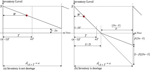
From (3), $f_{{\left.A\right|}_{A>T}}(a)=\mu e^{-\mu \left(a-T\right)}$ and the above equation yields:

(10) $\begin{array}{rl}& E\left[D{C}^{\left\{2\right\}}\right]=\frac{C_H\left(S-DT\right)}{\mu }+\frac{C_{H}D}{{\mu }^2}\left(e^{-\mu \left(\frac{S-DT}{D}\right)}-1\right)+\frac{C_{H}T\left(2S-DT\right)}{2}\\ & +\left(\frac{C_S\left(1-\beta \right)D{e}^{-\mu \left(\frac{S-DT}{D}\right)}}{\mu }\right)+\left(\frac{C_B\beta D{e}^{-\mu \left(\frac{S-DT}{D}\right)}}{{\mu }^2}\right)\end{array}$(10)

3.1.2.3. Optimal base stock level for the case$i=2$

Substitute $E\left[N\right]$, $E\left[{\left.A\right|}_{A>T}\right]$, $E\left[ND{C}^{\left\{2\right\}}\right]$, and $E\left[D{C}^{\left\{2\right\}}\right]$ derived in (2), (4), (9), and (10), respectively, for each corresponding component in (8), $E\left[TC{U}^{\left\{2\right\}}\left(S\right)\right]$ can be determined as:

$E\left[TC{U}^{\left\{2\right\}}\left(S\right)\right]=\frac{E\left[ND{C}^{\left\{2\right\}}\right]\left(E\left[N\right]-1\right)+E\left[D{C}^{\left\{2\right\}}\right]}{T\left(E\left[N\right]-1\right)+E\left[{\left.A\right|}_{A>T}\right]}=\frac{\left(\frac{C_{H}T\left(2S-DT\right)}{2}\right)\left(\left(\frac{1}{1-e^{-\lambda T}}\right)-1\right)+\left[\begin{array}{c}\frac{C_H\left(S-DT\right)}{\mu }+\frac{C_{H}D}{{\mu }^2}\left(e^{-\mu \left(\frac{S-DT}{D}\right)}-1\right)+\frac{C_{H}T\left(2S-DT\right)}{2}\\ +\left(\frac{C_S\left(1-\beta \right)D{e}^{-\mu \left(\frac{S-DT}{D}\right)}}{\mu }\right)+\left(\frac{C_B\beta D{e}^{-\mu \left(\frac{S-DT}{D}\right)}}{{\mu }^2}\right)\end{array}\right]}{T\left(\left(\frac{1}{1-e^{-\lambda T}}\right)-1\right)+\left(T+\frac{1}{\mu }\right)}$

Finally, we have:

(11) $E\left[TC{U}^{\left\{2\right\}}\left(S\right)\right]=\frac{\left[\begin{array}{c}\frac{C_H\left(S-DT\right)}{\mu }+\frac{C_{H}D}{{\mu }^2}\left(e^{-\mu \left(\frac{S-DT}{D}\right)}-1\right)+\frac{C_{H}T\left(2S-DT\right)}{2\left(1-e^{-\lambda T}\right)}\\ +\left(\frac{C_S\left(1-\beta \right)D{e}^{-\mu \left(\frac{S-DT}{D}\right)}}{\mu }\right)+\left(\frac{C_B\beta D{e}^{-\mu \left(\frac{S-DT}{D}\right)}}{{\mu }^2}\right)\end{array}\right]}{\left(\frac{T}{1-e^{-\lambda T}}+\frac{1}{\mu }\right)}$(11)

Then, the expression of $S^{\ast \left\{2\right\}}$ and the proof of convexity function are determined by Proposition 2.

Figure 4. Flow chart of solution method.

Proposition 2.

(i) $E\left[TC{U}^{\left\{2\right\}}\left(S\right)\right]$ is convex in $S$;

(ii) $S^{\ast \left\{2\right\}}=DT-\frac{Dln\left(\frac{C_H\left(\frac{T}{1-e^{-\lambda T}}+\frac{1}{\mu }\right)}{\frac{C_H}{\mu }+\frac{\beta C_B}{\mu }+\left(1-\beta \right)C_S}\right)}{\mu }$

Proof.

(i) $\frac{d^{2}E\left[TC{U}^{\left\{2\right\}}\left(S\right)\right]}{d{S}^2}=\frac{\left(C_H+\beta C_B+\mu \left(1-\beta \right)C_S\right)e^{-\mu \left(\frac{S-DT}{D}\right)}}{D\left(\frac{T}{\left(1-e^{-\lambda T}\right)}+\frac{1}{\mu }\right)}>0$.

Therefore, $E\left[TCU{\left(S\right)}^{\left\{2\right\}}\right]$ is convex in $S$□

(ii) $\begin{array}{rl}& \frac{dE\left[TC{U}^{\left\{2\right\}}\left(S^{\ast \left\{2\right\}}\right)\right]}{dS}\\ & =\frac{\left[C_H\left(\frac{T}{\left(1-e^{-\lambda T}\right)}+\frac{1}{\mu }\left(1-e^{\left(-\frac{\mu \left(S^{\ast \left\{2\right\}}-DT\right)}{D}\right)}\right)\right)-\left(\beta C_B+\left(1-\beta \right)C_S\right)e^{\left(-\frac{\mu \left(S^{\ast \left\{2\right\}}-DT\right)}{D}\right)}\right]}{\left(\frac{T}{1-e^{-\lambda T}}+\frac{1}{\mu }\right)}=0\end{array}$.

$S^{\ast \left\{2\right\}}=DT-\frac{Dln\left(\frac{C_H\left(\frac{T}{1-e^{-\lambda T}}+\frac{1}{\mu }\right)}{\frac{C_H}{\mu }+\frac{\beta C_B}{\mu }+\left(1-\beta \right)C_S}\right)}{\mu }$

□

3.2. Solution method to manifest the correct expression of optimal base stock level

In the above subsections, we determined the expressions for the optimal base stock level of two possible scenarios of a renewal cycle. However, given a set of parameter values, we still do not know whether the first or the second scenario will happen and which of the formulas should be used. In this section, we draw a solution method so that the corresponding expression of the optimal base stock level can be employed properly, namely, $S^{\ast \left\{1\right\}}$ or $S^{\ast \left\{2\right\}}$.

To begin with, Proposition 1 and Proposition 2 reveal that both $E\left[TC{U}^{\left\{1\right\}}\left(S\right)\right]$ and $E\left[TC{U}^{\left\{2\right\}}\left(S\right)\right]$ are convex functions in $S$. Because the correct use of $S^{\ast }$’s expression depends on the value of $DT$, which is the changing point for identifying the right scenario of a renewal cycle, we will examine $E\left[TC{U}^{\left\{1\right\}}\left(S\right)\right]$ and $E\left[TC{U}^{\left\{2\right\}}\left(S\right)\right]$ when $S=DT$, and the following proposition holds.

Proposition 3. If $S=DT$, $E\left[TC{U}^{\left\{1\right\}}\left(DT\right)\right]=E\left[TC{U}^{\left\{2\right\}}\left(DT\right)\right]$.

Proof.

From (7), $E\left[TC{U}^{\left\{1\right\}}\left(DT\right)\right]$ can be determined as:

$E\left[TC{U}^{\left\{1\right\}}\left(S\right)\right]=\frac{\left[\begin{array}{c}\left(\frac{C_H{S}^2}{2D}+\frac{C_B\beta {\left(DT-S\right)}^2}{2D}+C_S\left(1-\beta \right)\left(DT-S\right)\right)\left(\frac{e^{-\lambda T}}{1-e^{-\lambda T}}\right)\\ +\left(\begin{array}{c}\frac{C_H{S}^2}{2D}+C_B\beta \left(\frac{D{T}^2}{2}+\frac{S^2}{2D}+\left(T+\frac{1}{\mu }\right)\left(\frac{D}{\mu }-S\right)\right)\\ +C_S\left(1-\beta \right)\left(D\left(T+\frac{1}{\mu }\right)-S\right)\end{array}\right)\end{array}\right]}{\left(\frac{T}{1-e^{-\lambda T}}+\frac{1}{\mu }\right)}$

$E\left[TC{U}^{\left\{1\right\}}\left(DT\right)\right]=\frac{\left[\begin{array}{c}\left(\frac{C_H{\left(DT\right)}^2}{2D}+\frac{C_B\beta {\left(DT-DT\right)}^2}{2D}+C_S\left(1-\beta \right)\left(DT-DT\right)\right)\left(\frac{e^{-\lambda T}}{1-e^{-\lambda T}}\right)\\ +\left(\begin{array}{c}\frac{C_H{\left(DT\right)}^2}{2D}+C_B\beta \left(\frac{D{T}^2}{2}+\frac{{\left(DT\right)}^2}{2D}+\left(T+\frac{1}{\mu }\right)\left(\frac{D}{\mu }-\left(DT\right)\right)\right)\\ +C_S\left(1-\beta \right)\left(D\left(T+\frac{1}{\mu }\right)-\left(DT\right)\right)\end{array}\right)\end{array}\right]}{\left(\frac{T}{1-e^{-\lambda T}}+\frac{1}{\mu }\right)}$

Finally,

$E\left[TC{U}^{\left\{1\right\}}\left(DT\right)\right]=\frac{\left[\left(\frac{C_{H}D{T}^2}{2\left(1-e^{-\lambda T}\right)}\right)+\frac{C_B\beta D}{{\mu }^2}+\frac{C_S\left(1-\beta \right)D}{\mu }\right]}{\left(\frac{T}{1-e^{-\lambda T}}+\frac{1}{\mu }\right)}$

Also, from (11), $E\left[TC{U}^{\left\{2\right\}}\left(DT\right)\right]$ can be determined as:

$E\left[TC{U}^{\left\{2\right\}}\left(S\right)\right]=\frac{\left[\begin{array}{c}\frac{C_H\left(S-DT\right)}{\mu }+\frac{C_{H}D}{{\mu }^2}\left(e^{-\mu \left(\frac{S-DT}{D}\right)}-1\right)+\frac{C_{H}T\left(2S-DT\right)}{2\left(1-e^{-\lambda T}\right)}\\ +\left(\frac{C_S\left(1-\beta \right)D{e}^{-\mu \left(\frac{S-DT}{D}\right)}}{\mu }\right)+\left(\frac{C_B\beta D{e}^{-\mu \left(\frac{S-DT}{D}\right)}}{{\mu }^2}\right)\end{array}\right]}{\left(\frac{T}{1-e^{-\lambda T}}+\frac{1}{\mu }\right)}$

$E\left[TC{U}^{\left\{2\right\}}\left(DT\right)\right]=\frac{\left[\begin{array}{c}\frac{C_H\left(DT-DT\right)}{\mu }+\frac{C_{H}D}{{\mu }^2}\left(e^{-\mu \left(\frac{DT-DT}{D}\right)}-1\right)+\frac{C_{H}T\left(2DT-DT\right)}{2\left(1-e^{-\lambda T}\right)}\\ +\left(\frac{C_S\left(1-\beta \right)D{e}^{-\mu \left(\frac{DT-DT}{D}\right)}}{\mu }\right)+\left(\frac{C_B\beta D{e}^{-\mu \left(\frac{DT-DT}{D}\right)}}{{\mu }^2}\right)\end{array}\right]}{\left(\frac{T}{1-e^{-\lambda T}}+\frac{1}{\mu }\right)}$

Finally,

$E\left[TC{U}^{\left\{2\right\}}\left(DT\right)\right]=\frac{\left[\left(\frac{C_{H}D{T}^2}{2\left(1-e^{-\lambda T}\right)}\right)+\frac{C_S\left(1-\beta \right)D}{\mu }+\frac{C_B\beta D}{{\mu }^2}\right]}{\left(\frac{T}{1-e^{-\lambda T}}+\frac{1}{\mu }\right)}$

□

At $S=DT$, $E\left[TC{U}^{\left\{1\right\}}\left(DT\right)\right]=E\left[TC{U}^{\left\{2\right\}}\left(DT\right)\right]$

Proposition 3 leads to the fact that the functions of $E\left[TC{U}^{\left\{1\right\}}\left(DT\right)\right]$ and $E\left[TC{U}^{\left\{2\right\}}\left(DT\right)\right]$ can follow any patterns; however, both $E\left[TC{U}^{\left\{1\right\}}\left(DT\right)\right]$ and $E\left[TC{U}^{\left\{2\right\}}\left(DT\right)\right]$ result in the same value of the expected costs per day at $S=DT$.

For the sake of reasonableness, $S^{\ast \left\{1\right\}}<DT$ and $S^{\ast \left\{2\right\}}>DT$. If only one of them holds true, it is possible to determine the correct expression for the optimal base stock level. However, if both of them hold true, a difficulty arises. Following, various cases are analyzed: $S^{\ast \left\{1\right\}}<DT$ and $S^{\ast \left\{2\right\}}>DT$, $S^{\ast \left\{1\right\}}>DT$ and $S^{\ast \left\{2\right\}}<DT$, $S^{\ast \left\{1\right\}}$ or $S^{\ast \left\{2\right\}}=DT$.

Proposition 4. It is impossible that the situation $S^{\ast \left\{1\right\}}<DT$ and $S^{\ast \left\{2\right\}}>DT$ will occur simultaneously.

Proof.

Substitute the expression of $S^{\ast \left\{1\right\}}$ into $S^{\ast \left\{1\right\}}<DT$, we have:

$\frac{C_S\left(1-\beta \right)}{1-e^{-\lambda T}}+\frac{\beta C_B}{\mu }<\frac{T{C}_H}{1-e^{-\lambda T}}$

As with above, substitute the expression of $S^{\ast \left\{2\right\}}$ into $S^{\ast \left\{2\right\}}>DT$, we have:

$C_S\left(1-\beta \right)+\frac{\beta C_B}{\mu }>\frac{T{C}_H}{1-e^{-\lambda T}}$

Due to the fact that $\frac{C_S\left(1-\beta \right)}{1-e^{-\lambda T}}+\frac{\beta C_B}{\mu }\ge C_S\left(1-\beta \right)+\frac{\beta C_B}{\mu }$ and the situation $S^{\ast \left\{1\right\}}<DT$ and $S^{\ast \left\{2\right\}}>DT$ will not occur simultaneously.□

Proposition 4 provides the fact that only either $S^{\ast \left\{1\right\}}<DT$ or $S^{\ast \left\{2\right\}}>DT$ holds true for a given set of parameters value. Therefore, in case both $S^{\ast \left\{1\right\}}<DT$ and $S^{\ast \left\{2\right\}}<DT$, the correct expression follows $S^{\ast \left\{1\right\}}$ (because $S^{\ast \left\{2\right\}}$ cannot be less than $DT$). Also, in case both $S^{\ast \left\{1\right\}}>DT$ and $S^{\ast \left\{2\right\}}>DT$, the correct expression follows $S^{\ast \left\{2\right\}}$ (because $S^{\ast \left\{1\right\}}$ cannot be greater than $DT$).

For the case both $S^{\ast \left\{1\right\}}>DT$ and $S^{\ast \left\{2\right\}}<DT$, the correct expression for the optimal base stock level has not been addressed. Proposition 5 helps derive the correct expression for the case.

Proposition 5.

(i) If $S^{\ast \left\{1\right\}}>DT$ and $S^{\ast \left\{2\right\}}<DT$, the expression for optimal base stock level is $S^{\ast }=DT$;

(ii) The parameters’ values leading to the condition $S^{\ast \left\{1\right\}}>DT$ and $S^{\ast \left\{2\right\}}<DT$ must satisfy $C_S\left(1-\beta \right)+\frac{\beta C_B}{\mu }<\frac{T{C}_H}{1-e^{-\lambda T}}<\frac{C_S\left(1-\beta \right)}{1-e^{-\lambda T}}+\frac{\beta C_B}{\mu }$.

Proof.

Both $S^{\ast \left\{1\right\}}>DT$ and $S^{\ast \left\{2\right\}}<DT$ are infeasible. $E\left[TC{U}^{\left\{1\right\}}\left(S\right)\right]$ is the effective expression addressing the total cost per time unit for $0\le S<DT$ while $E\left[TC{U}^{\left\{2\right\}}\left(S\right)\right]$ is the effective expression for $S>DT$. For $S=DT$, both $E\left[TC{U}^{\left\{1\right\}}\left(S\right)\right]$ and $E\left[TC{U}^{\left\{2\right\}}\left(S\right)\right]$ are effective, as illustrated in Proposition 3. Considering the characteristics of $E\left[TC{U}^{\left\{1\right\}}\left(S\right)\right]$ and $E\left[TC{U}^{\left\{2\right\}}\left(S\right)\right]$ in this case, $E\left[TC{U}^{\left\{1\right\}}\left(S\right)\right]$ decreases when $S$ increases for $0\le S\le DT$, due to $S^{\ast \left\{1\right\}}>DT$, and $E\left[TC{U}^{\left\{2\right\}}\left(S\right)\right]$ increases when $S$ increases for $S>DT$, due to $S^{\ast \left\{2\right\}}<DT$. Therefore, $DT$ is the optimal base stock level and, according to Proposition 3, $E\left[TC{U}^{\left\{1\right\}}\left(DT\right)\right]=E\left[TC{U}^{\left\{2\right\}}\left(DT\right)\right]$.□

Substitute the expression of $S^{\ast \left\{1\right\}}$ into $S^{\ast \left\{1\right\}}>DT$, we have:

$\frac{C_S\left(1-\beta \right)}{1-e^{-\lambda T}}+\frac{\beta C_B}{\mu }>\frac{T{C}_H}{1-e^{-\lambda T}}$

As with above, substitute the expression of $S^{\ast \left\{2\right\}}$ into $S^{\ast \left\{2\right\}}<DT$, we have:

$C_S\left(1-\beta \right)+\frac{\beta C_B}{\mu }<\frac{T{C}_H}{1-e^{-\lambda T}}$

Therefore, the parameters’ values leading to the condition $S^{\ast \left\{1\right\}}>DT$ and $S^{\ast \left\{2\right\}}<DT$ must satisfy $C_S\left(1-\beta \right)+\frac{\beta C_B}{\mu }<\frac{T{C}_H}{1-e^{-\lambda T}}<\frac{C_S\left(1-\beta \right)}{1-e^{-\lambda T}}+\frac{\beta C_B}{\mu }$.□

Next, in order to examine whether the cases $S^{\ast \left\{1\right\}}=DT$ and $S^{\ast \left\{2\right\}}>DT$; or $S^{\ast \left\{2\right\}}=DT$ and $S^{\ast \left\{1\right\}}<DT$ will not occur, the following proposition holds.

Proposition 6.

(i) If $S^{\ast \left\{1\right\}}=DT$, the condition under which $S^{\ast \left\{1\right\}}=DT$ leads to the fact that $S^{\ast \left\{2\right\}}\le DT$. However, $S^{\ast \left\{2\right\}}<DT$ is infeasible. Therefore, the optimal base stock level is $S^{\ast }=DT$;

(ii) If $S^{\ast \left\{2\right\}}=DT$, the condition under which $S^{\ast \left\{2\right\}}=DT$ leads to the fact that $S^{\ast \left\{1\right\}}\ge DT$. However, $S^{\ast \left\{1\right\}}>DT$ is infeasible. Therefore, the optimal base stock level is $S^{\ast }=DT$.

Proof.

(i) From a proof of Proposition 4, the condition under which $S^{\ast \left\{1\right\}}=DT$ is $\frac{\beta C_B}{\mu }=\frac{T{C}_H}{1-e^{-\lambda T}}-\frac{C_S\left(1-\beta \right)}{1-e^{-\lambda T}}$. Replacing $\frac{\beta C_B}{\mu }$ into the expression of $S^{\ast \left\{2\right\}}$, we have:

$S^{\ast \left\{2\right\}}=DT-\frac{Dln\left(\frac{\frac{C_{H}T}{1-e^{-\lambda T}}+\frac{C_H}{\mu }}{\frac{C_H}{\mu }+\frac{C_{H}T}{1-e^{-\lambda T}}-C_S\left(1-\beta \right)\left(\frac{1}{1-e^{-\lambda T}}-1\right)}\right)}{\mu }$

Because $\left(\frac{1}{1-e^{-\lambda T}}-1\right)\ge 0$. Therefore, $ln\left(\frac{\frac{C_{H}T}{1-e^{-\lambda T}}+\frac{C_H}{\mu }}{\frac{C_H}{\mu }+\frac{C_{H}T}{1-e^{-\lambda T}}-C_S\left(1-\beta \right)\left(\frac{1}{1-e^{-\lambda T}}-1\right)}\right)\ge 0$ and $S^{\ast \left\{2\right\}}\le DT$.□

(ii) From a proof of Proposition 4, the condition under which $S^{\ast \left\{2\right\}}=DT$ is $\frac{\beta C_B}{\mu }=\frac{T{C}_H}{1-e^{-\lambda T}}-C_S\left(1-\beta \right)$. Replacing $\frac{\beta C_B}{\mu }$ into the expression of $S^{\ast \left\{1\right\}}$, we have:

$S^{\ast \left\{1\right\}}=D\left(T+\left(\frac{C_S\left(1-\beta \right)e^{-\lambda T}}{C_H+C_B\beta }\right)\right)$

Because $\left(\frac{C_S\left(1-\beta \right)e^{-\lambda T}}{C_H+C_B\beta }\right)\ge 0$. Therefore, $S^{\ast \left\{1\right\}}\ge DT$.□

In order to draw the solution method, the following are performed. First, $S^{\ast \left\{1\right\}}$ and $S^{\ast \left\{2\right\}}$ are computed using Proposition 1 and Proposition 2, respectively. According to Proposition 4, $S^{\ast }=S^{\ast \left\{1\right\}}$ if $S^{\ast \left\{1\right\}}<DT$; and $S^{\ast }=S^{\ast \left\{2\right\}}$ if $S^{\ast \left\{2\right\}}>DT$. If both $S^{\ast \left\{1\right\}}>DT$ and $S^{\ast \left\{2\right\}}<DT$, $S^{\ast }=DT$, according to Proposition 5; and $E\left[TCU\left(S^{\ast }\right)\right]=E\left[TC{U}^{\left\{1\right\}}\left(DT\right)\right]=E\left[TC{U}^{\left\{2\right\}}\left(DT\right)\right]$, according to Proposition 3. According to Proposition 6, if either $S^{\ast \left\{1\right\}}=DT$ or $S^{\ast \left\{2\right\}}=DT$, $S^{\ast }=DT$. The following figure summarizes the proposed solution method to derive the optimal base stock level as well as the minimum cost per time unit, as seen in Figure 4.

4. Numerical experiments

The main purpose of this section is to illustrate the applicability of the proposed solution method. First, the following values of parameters are assumed and referred to as base case: $D=5$ units per day, $T=10$days $C_H=1$$ per unit per day, $C_S=20$$ per unit, $C_B=5$$ per unit per day, $\lambda =0.05$times per day, $\mu =0.1$times per day, $\beta =0.5$. Subject to the values of parameters, $S^{\ast \left\{1\right\}}=64.05$ units, and $S^{\ast \left\{2\right\}}=61.98$ units. According to the flow chart of the solution method, $S^{\ast }=S^{\ast \left\{2\right\}}=61.98$ units and the corresponding $E\left[TCU\left(S^{\ast }\right)\right]=E\left[TC{U}^{\left\{2\right\}}\left(S^{\ast }\right)\right]=65.80$ $ per day. Next, we will conduct sensitivity analyses.

The optimal base stock level and minimum cost per day for various values of $\beta$, $\lambda$, and $\mu$ are shown in Appendix A (Table A1-A4). As expected, the increase in the value of $\mu$ decreases the optimal base stock level and the corresponding minimum cost per day decreases. On the other hand, the increase in the value of $\lambda$ increases the optimal base stock level, and the corresponding minimum cost per day also increases. These trends make sense because a higher value of $\mu$ means that the mean of disruption length is shorter, and a higher value of $\lambda$ leads to the fact that the supply disruption is more likely to occur.

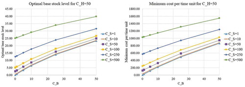
Changing the value of cost parameters ($C_S$, $C_B$, $C_H$), we will examine the behavior of the proposed model. The optimal base stock level and minimum cost per day for various values of cost parameters are shown in Appendix B (Figure B1-B6). It can be seen that $E\left[TCU\left(S^{\ast }\right)\right]$ increases as the value of cost parameters increases. Regarding the effect of changing in $C_H$ value on $S^{\ast }$, the increase in $C_H$ value usually causes the decrease in $S^{\ast }$; and the special cases where the increase in $C_H$ value does not change $S^{\ast }$ will be discussed later. Examining the effect of shortage inventory costs ($C_S$, $C_B$) on $S^{\ast }$, the increase in $C_S$ value usually causes the increase in $S^{\ast }$; likewise, the increase in $C_B$ value usually causes the increase in $S^{\ast }$. The main reason for the behavior is that the retailer should prevent excessive shortage inventory costs by increasing the base stock level as the shortage inventory costs increases. For those cases that the increase in holding costs and shortage costs does not change $S^{\ast }$, the parameters’ values leading to the cases satisfy the condition proposed in Proposition 5. Therefore, there exist some cases that the optimal base stock level is insensitive to the changing in the value of cost parameters.

All in all, it can be confirmed that the optimal level of base stock and the corresponding minimum cost per day can always be determined. The proposed solution method helps managers derive the optimal level of base stock conveniently. Regarding the effect of changing in the value of important parameters, the retailer should increase the level of base stock in the presence of the increase in disruption frequency or the increase in disruption length. Usually, the retailer should decrease the base stock level as the holding costs increases; and the retailer should increase the base stock level as the shortage costs increases. The cases that the base stock level is insensitive to the changing in the value of cost parameters can also be detected.

5. Conclusions

In this research work, inventory holding is used to cope with a supply disruption problem. Under a periodic review base stock system, the retailer is supposed to determine the optimal base stock level, which helps minimize the costs per unit of time. The retailer’s expected cost per unit of time function is formulated, and all possible scenarios of a renewal cycle, as well as the associated costs, are analyzed. The current research work is distinguished from the existing literature as it uses a continuous variable of the disruption length together with partial backorder to derive the closed-form expression for the optimal base stock level. A solution method is proposed in order to derive the correct expression for the optimal base stock level as well as the minimum costs per unit of time. In the numerical experiment section, we investigate the behaviors of the system for various values of input parameters through the use of the proposed structural result. It can be confirmed that the optimal base stock level, which minimizes the costs per unit of time, can always be determined. Complementary to the finding, the optimal base stock level for some cases are found to be insensitive to the changing in value of cost parameters. From a managerial perspective, since the closed-form expression is derived and the optimal base stock level can be easily computed through a few steps, the proposed solution method helps managers obtain it precisely and conveniently in the presence of stochastic supply disruption. Despite the merits, the assumption of deterministic demand is assumed in this research work, and it could be relaxed by considering stochastic demand. The derivation of an approximate/exact closed-form expression for the optimal base stock level by considering the continuous variable of the disruption length, partial backorder, and stochastic demand has not been examined before. Therefore, we note this vacant issue as a further research topic.

Additional information

Funding

The authors received no direct funding for this research.

Notes on contributors

Chirakiat Saithong

Chirakiat Saithong is currently a lecturer in the Department of Industrial Engineering, Faculty of Engineering at Sriracha, Kasetsart University Sriracha Campus, Thailand. He received Doctor of Engineering (D.Eng) from the Asian Institute of Technology, Thailand, in 2018. His research interest is in analyzing uncertainties in supply chains.

Saowanit Lekhavat

Saowanit Lekhavat is a lecturer at the Faculty of Logistics, Burapha University. She received her Ph.D. in Operational Research from Brunel University London. Her research interests are maritime transport, location-allocation problem, simulation, optimization, meta-heuristics algorithm, and lean manufacturing.

Appendix A.

Table A1. Optimal base stock level and minimum cost per day for $\beta$= 1.00

$\beta$	$\lambda$	$\mu$	$S^{\ast \left\{1\right\}}$	$S^{\ast \left\{2\right\}}$	$E\left[TC{U}^{\left\{1\right\}}\left(S^{\ast \left\{1\right\}}\right)\right]$	$E\left[TC{U}^{\left\{2\right\}}\left(S^{\ast \left\{2\right\}}\right)\right]$	$S^{\ast }$	$E\left[TCU\left(S^{\ast }\right)\right]$
1.00	0.01	0.05	49.60	45.85	100.94	100.86	49.60	100.94
1.00	0.01	0.10	45.63	17.43	43.51	35.92	45.63	43.51
1.00	0.01	0.50	42.46	28.11	22.12	12.46	42.46	22.12
1.00	0.01	1.00	42.06	35.64	21.26	15.35	42.06	21.26
1.00	0.01	5.00	41.75	45.53	20.88	21.48	41.75	20.88
1.00	0.01	10.00	41.71	47.42	20.86	22.89	41.71	20.86
1.00	0.01	20.00	41.69	48.54	20.84	23.77	41.69	20.84
1.00	0.05	0.05	74.46	147.17	214.10	167.12	147.17	167.12
1.00	0.05	0.10	58.06	76.36	85.73	80.18	76.36	80.18
1.00	0.05	0.50	44.95	41.74	25.40	24.18	44.95	25.40
1.00	0.05	1.00	43.31	42.59	22.41	21.45	43.31	22.41
1.00	0.05	5.00	41.99	46.94	21.03	22.74	41.99	21.03
1.00	0.05	10.00	41.83	48.12	20.92	23.53	41.83	20.92
1.00	0.05	20.00	41.75	48.89	20.88	24.09	41.75	20.88
1.00	0.10	0.05	94.34	170.90	238.11	176.11	170.90	176.11
1.00	0.10	0.10	68.01	92.16	100.23	88.11	92.16	88.11
1.00	0.10	0.50	46.93	46.05	27.31	27.12	46.93	27.31
1.00	0.10	1.00	44.30	44.85	23.17	23.06	44.30	23.17
1.00	0.10	5.00	42.19	47.41	21.14	23.08	42.19	21.14
1.00	0.10	10.00	41.93	48.36	20.98	23.70	41.93	20.98
1.00	0.10	20.00	41.80	49.01	20.90	24.18	41.80	20.90
1.00	0.50	0.05	124.44	188.40	229.63	180.26	188.40	180.26
1.00	0.50	0.10	83.05	104.76	104.23	92.39	104.76	92.39
1.00	0.50	0.50	49.94	49.94	29.14	29.14	49.94	29.14
1.00	0.50	1.00	45.81	46.94	24.04	24.23	45.81	24.04
1.00	0.50	5.00	42.49	47.85	21.30	23.35	42.49	21.30
1.00	0.50	10.00	42.08	48.58	21.05	23.83	42.08	21.05
1.00	0.50	20.00	41.87	49.12	20.94	24.25	41.87	20.94
1.00	1.00	0.05	125.00	188.63	229.17	180.30	188.63	180.30
1.00	1.00	0.10	83.33	104.93	104.17	92.43	104.93	92.43
1.00	1.00	0.50	50.00	50.00	29.17	29.17	50.00	29.17
1.00	1.00	1.00	45.83	46.97	24.05	24.24	45.83	24.05
1.00	1.00	5.00	42.50	47.86	21.30	23.35	42.50	21.30
1.00	1.00	10.00	42.08	48.59	21.05	23.84	42.08	21.05
1.00	1.00	20.00	41.87	49.12	20.94	24.25	41.87	20.94
1.00	5.00	0.05	125.00	188.63	229.17	180.30	188.63	180.30
1.00	5.00	0.10	83.33	104.93	104.17	92.43	104.93	92.43
1.00	5.00	0.50	50.00	50.00	29.17	29.17	50.00	29.17
1.00	5.00	1.00	45.83	46.97	24.05	24.24	45.83	24.05
1.00	5.00	5.00	42.50	47.86	21.30	23.35	42.50	21.30
1.00	5.00	10.00	42.08	48.59	21.05	23.84	42.08	21.05
1.00	5.00	20.00	41.88	49.12	20.94	24.25	41.88	20.94
1.00	10.00	0.05	125.00	188.63	229.17	180.30	188.63	180.30
1.00	10.00	0.10	83.33	104.93	104.17	92.43	104.93	92.43
1.00	10.00	0.50	50.00	50.00	29.17	29.17	50.00	29.17
1.00	10.00	1.00	45.83	46.97	24.05	24.24	45.83	24.05
1.00	10.00	5.00	42.50	47.86	21.30	23.35	42.50	21.30
1.00	10.00	10.00	42.08	48.59	21.05	23.84	42.08	21.05
1.00	10.00	20.00	41.88	49.12	20.94	24.25	41.88	20.94

Table A2. Optimal base stock level and minimum cost per day for $\beta$= 0.50

$\beta$	$\lambda$	$\mu$	$S^{\ast \left\{1\right\}}$	$S^{\ast \left\{2\right\}}$	$E\left[TC{U}^{\left\{1\right\}}\left(S^{\ast \left\{1\right\}}\right)\right]$	$E\left[TC{U}^{\left\{2\right\}}\left(S^{\ast \left\{2\right\}}\right)\right]$	$S^{\ast }$	$E\left[TCU\left(S^{\ast }\right)\right]$
0.50	0.01	0.05	56.80	5.30	67.61	60.32	50.00	67.61
0.50	0.01	0.10	53.40	3.05	37.66	21.53	50.00	37.66
0.50	0.01	0.50	50.68	31.60	25.92	15.94	50.00	25.92
0.50	0.01	1.00	50.34	39.69	25.35	19.41	50.00	25.35
0.50	0.01	5.00	50.07	47.71	25.05	23.66	50.00	25.05
0.50	0.01	10.00	50.03	48.84	25.02	24.32	50.00	25.02
0.50	0.01	20.00	50.02	49.42	25.01	24.65	50.00	25.01
0.50	0.05	0.05	78.10	106.62	130.63	126.57	106.62	126.57
0.50	0.05	0.10	64.05	61.98	62.40	65.80	61.98	65.80
0.50	0.05	0.50	52.81	45.22	28.39	27.67	50.00	28.39
0.50	0.05	1.00	51.41	46.64	26.35	25.51	50.00	26.35
0.50	0.05	5.00	50.28	49.13	25.21	24.92	50.00	25.21
0.50	0.05	10.00	50.14	49.55	25.10	24.95	50.00	25.10
0.50	0.05	20.00	50.07	49.77	25.05	24.97	50.00	25.05
0.50	0.10	0.05	95.15	130.35	147.03	135.56	130.35	135.56
0.50	0.10	0.10	72.58	77.78	72.17	73.73	77.78	73.73
0.50	0.10	0.50	54.52	49.53	29.98	30.60	50.00	29.98
0.50	0.10	1.00	52.26	48.90	27.06	27.12	50.00	27.06
0.50	0.10	5.00	50.45	49.60	25.34	25.27	50.00	25.34
0.50	0.10	10.00	50.23	49.78	25.16	25.12	50.00	25.16
0.50	0.10	20.00	50.11	49.89	25.08	25.06	50.00	25.08
0.50	0.50	0.05	120.95	147.86	148.93	139.71	147.86	139.71
0.50	0.50	0.10	85.47	90.38	77.65	78.00	90.38	78.00
0.50	0.50	0.50	57.09	53.43	31.82	32.63	53.43	32.63
0.50	0.50	1.00	53.55	50.99	27.99	28.28	50.99	28.28
0.50	0.50	5.00	50.71	50.04	25.52	25.53	50.04	25.53
0.50	0.50	10.00	50.35	50.01	25.25	25.26	50.01	25.26
0.50	0.50	20.00	50.18	50.00	25.13	25.13	50.00	25.13
0.50	1.00	0.05	121.43	148.08	148.81	139.75	148.08	139.75
0.50	1.00	0.10	85.71	90.55	77.68	78.05	90.55	78.05
0.50	1.00	0.50	57.14	53.48	31.85	32.65	53.48	32.65
0.50	1.00	1.00	53.57	51.02	28.00	28.30	51.02	28.30
0.50	1.00	5.00	50.71	50.05	25.52	25.54	50.05	25.54
0.50	1.00	10.00	50.36	50.01	25.26	25.26	50.01	25.26
0.50	1.00	20.00	50.18	50.00	25.13	25.13	50.00	25.13
0.50	5.00	0.05	121.43	148.08	148.81	139.75	148.08	139.75
0.50	5.00	0.10	85.71	90.55	77.68	78.05	90.55	78.05
0.50	5.00	0.50	57.14	53.48	31.85	32.65	53.48	32.65
0.50	5.00	1.00	53.57	51.02	28.00	28.30	51.02	28.30
0.50	5.00	5.00	50.71	50.05	25.52	25.54	50.05	25.54
0.50	5.00	10.00	50.36	50.01	25.26	25.26	50.01	25.26
0.50	5.00	20.00	50.18	50.00	25.13	25.13	50.00	25.13
0.50	10.00	0.05	121.43	148.08	148.81	139.75	148.08	139.75
0.50	10.00	0.10	85.71	90.55	77.68	78.05	90.55	78.05
0.50	10.00	0.50	57.14	53.48	31.85	32.65	53.48	32.65
0.50	10.00	1.00	53.57	51.02	28.00	28.30	51.02	28.30
0.50	10.00	5.00	50.71	50.05	25.52	25.54	50.05	25.54
0.50	10.00	10.00	50.36	50.01	25.26	25.26	50.01	25.26
0.50	10.00	20.00	50.18	50.00	25.13	25.13	50.00	25.13

Table A3. Optimal base stock level and minimum cost per day for $\beta$= 0.10

$\beta$	$\lambda$	$\mu$	$S^{\ast \left\{1\right\}}$	$S^{\ast \left\{2\right\}}$	$E\left[TC{U}^{\left\{1\right\}}\left(S^{\ast \left\{1\right\}}\right)\right]$	$E\left[TC{U}^{\left\{2\right\}}\left(S^{\ast \left\{2\right\}}\right)\right]$	$S^{\ast }$	$E\left[TCU\left(S^{\ast }\right)\right]$
0.10	0.01	0.05	79.84	−45.78	32.17	9.24	50.00	32.17
0.10	0.01	0.10	78.25	−12.46	21.89	6.03	50.00	21.89
0.10	0.01	0.50	76.98	33.71	15.59	18.06	50.00	15.59
0.10	0.01	1.00	76.83	41.53	14.94	21.25	50.00	14.94
0.10	0.01	5.00	76.70	48.25	14.45	24.20	50.00	14.45
0.10	0.01	10.00	76.68	49.12	14.39	24.60	50.00	14.39
0.10	0.01	20.00	76.67	49.56	14.36	24.80	50.00	14.36
0.10	0.05	0.05	89.78	55.54	62.36	75.49	55.54	75.49
0.10	0.05	0.10	83.22	46.47	38.53	50.29	50.00	38.53
0.10	0.05	0.50	77.98	47.33	19.22	29.78	50.00	19.22
0.10	0.05	1.00	77.32	48.48	16.78	27.35	50.00	16.78
0.10	0.05	5.00	76.80	49.66	14.82	25.46	50.00	14.82
0.10	0.05	10.00	76.73	49.83	14.58	25.23	50.00	14.58
0.10	0.05	20.00	76.70	49.91	14.46	25.11	50.00	14.46
0.10	0.10	0.05	97.74	79.27	74.11	84.48	79.27	84.48
0.10	0.10	0.10	87.20	62.27	47.14	58.22	62.27	58.22
0.10	0.10	0.50	78.77	51.64	21.83	32.71	51.64	32.71
0.10	0.10	1.00	77.72	50.74	18.17	28.96	50.74	28.96
0.10	0.10	5.00	76.88	50.13	15.12	25.81	50.13	25.81
0.10	0.10	10.00	76.77	50.07	14.73	25.41	50.07	25.41
0.10	0.10	20.00	76.72	50.03	14.53	25.20	50.03	25.20
0.10	0.50	0.05	109.78	96.77	83.55	88.63	96.77	88.63
0.10	0.50	0.10	93.22	74.87	55.79	62.50	74.87	62.50
0.10	0.50	0.50	79.98	55.54	25.36	34.74	55.54	34.74
0.10	0.50	1.00	78.32	52.83	20.15	30.12	52.83	30.12
0.10	0.50	5.00	77.00	50.58	15.56	26.07	50.58	26.07
0.10	0.50	10.00	76.83	50.29	14.95	25.54	50.29	25.54
0.10	0.50	20.00	76.75	50.15	14.64	25.27	50.15	25.27
0.10	1.00	0.05	110.00	97.00	83.67	88.67	97.00	88.67
0.10	1.00	0.10	93.33	75.04	55.92	62.54	75.04	62.54
0.10	1.00	0.50	80.00	55.60	25.42	34.76	55.60	34.76
0.10	1.00	1.00	78.33	52.86	20.19	30.14	52.86	30.14
0.10	1.00	5.00	77.00	50.58	15.56	26.07	50.58	26.07
0.10	1.00	10.00	76.83	50.29	14.95	25.54	50.29	25.54
0.10	1.00	20.00	76.75	50.15	14.64	25.27	50.15	25.27
0.10	5.00	0.05	110.00	97.00	83.67	88.67	97.00	88.67
0.10	5.00	0.10	93.33	75.04	55.92	62.54	75.04	62.54
0.10	5.00	0.50	80.00	55.60	25.42	34.76	55.60	34.76
0.10	5.00	1.00	78.33	52.86	20.19	30.14	52.86	30.14
0.10	5.00	5.00	77.00	50.58	15.56	26.07	50.58	26.07
0.10	5.00	10.00	76.83	50.29	14.95	25.54	50.29	25.54
0.10	5.00	20.00	76.75	50.15	14.64	25.27	50.15	25.27
0.10	10.00	0.05	110.00	97.00	83.67	88.67	97.00	88.67
0.10	10.00	0.10	93.33	75.04	55.92	62.54	75.04	62.54
0.10	10.00	0.50	80.00	55.60	25.42	34.76	55.60	34.76
0.10	10.00	1.00	78.33	52.86	20.19	30.14	52.86	30.14
0.10	10.00	5.00	77.00	50.58	15.56	26.07	50.58	26.07
0.10	10.00	10.00	76.83	50.29	14.95	25.54	50.29	25.54
0.10	10.00	20.00	76.75	50.15	14.64	25.27	50.15	25.27

Table A4. Optimal base stock level and minimum cost per day for $\beta$= 0.00

$\beta$	$\lambda$	$\mu$	$S^{\ast \left\{1\right\}}$	$S^{\ast \left\{2\right\}}$	$E\left[TC{U}^{\left\{1\right\}}\left(S^{\ast \left\{1\right\}}\right)\right]$	$E\left[TC{U}^{\left\{2\right\}}\left(S^{\ast \left\{2\right\}}\right)\right]$	$S^{\ast }$	$E\left[TCU\left(S^{\ast }\right)\right]$
0.00	0.01	0.05	100.00	−64.01	15.99	−9.00	50.00	15.99
0.00	0.01	0.10	100.00	−17.22	8.69	1.26	50.00	8.69
0.00	0.01	0.50	100.00	34.17	1.87	18.52	50.00	1.87
0.00	0.01	1.00	100.00	41.90	0.94	21.62	50.00	0.94
0.00	0.01	5.00	100.00	48.35	0.19	24.30	50.00	0.19
0.00	0.01	10.00	100.00	49.17	0.10	24.65	50.00	0.10
0.00	0.01	20.00	100.00	49.59	0.05	24.82	50.00	0.05
0.00	0.05	0.05	100.00	37.30	44.04	57.26	50.00	44.04
0.00	0.05	0.10	100.00	41.70	28.24	45.53	50.00	28.24
0.00	0.05	0.50	100.00	47.80	7.30	30.25	50.00	7.30
0.00	0.05	1.00	100.00	48.85	3.79	27.72	50.00	3.79
0.00	0.05	5.00	100.00	49.76	0.78	25.56	50.00	0.78
0.00	0.05	10.00	100.00	49.88	0.39	25.28	50.00	0.39
0.00	0.05	20.00	100.00	49.94	0.20	25.14	50.00	0.20
0.00	0.10	0.05	100.00	61.04	55.84	66.24	61.04	66.24
0.00	0.10	0.10	100.00	57.50	38.73	53.46	57.50	53.46
0.00	0.10	0.50	100.00	52.11	11.22	33.18	52.11	33.18
0.00	0.10	1.00	100.00	51.11	5.95	29.33	51.11	29.33
0.00	0.10	5.00	100.00	50.23	1.25	25.91	50.23	25.91
0.00	0.10	10.00	100.00	50.12	0.63	25.46	50.12	25.46
0.00	0.10	20.00	100.00	50.06	0.32	25.23	50.06	25.23
0.00	0.50	0.05	100.00	78.54	66.52	70.40	78.54	70.40
0.00	0.50	0.10	100.00	70.10	49.83	57.73	70.10	57.73
0.00	0.50	0.50	100.00	56.00	16.57	35.20	56.00	35.20
0.00	0.50	1.00	100.00	53.20	9.04	30.49	53.20	30.49
0.00	0.50	5.00	100.00	50.68	1.95	26.17	50.68	26.17
0.00	0.50	10.00	100.00	50.34	0.98	25.59	50.34	25.59
0.00	0.50	20.00	100.00	50.17	0.49	25.30	50.17	25.30
0.00	1.00	0.05	100.00	78.77	66.67	70.43	78.77	70.43
0.00	1.00	0.10	100.00	70.27	50.00	57.77	70.27	57.77
0.00	1.00	0.50	100.00	56.06	16.67	35.23	56.06	35.23
0.00	1.00	1.00	100.00	53.23	9.09	30.51	53.23	30.51
0.00	1.00	5.00	100.00	50.68	1.96	26.17	50.68	26.17
0.00	1.00	10.00	100.00	50.34	0.99	25.59	50.34	25.59
0.00	1.00	20.00	100.00	50.17	0.50	25.30	50.17	25.30
0.00	5.00	0.05	100.00	78.77	66.67	70.43	78.77	70.43
0.00	5.00	0.10	100.00	70.27	50.00	57.77	70.27	57.77
0.00	5.00	0.50	100.00	56.06	16.67	35.23	56.06	35.23
0.00	5.00	1.00	100.00	53.23	9.09	30.51	53.23	30.51
0.00	5.00	5.00	100.00	50.68	1.96	26.17	50.68	26.17
0.00	5.00	10.00	100.00	50.34	0.99	25.59	50.34	25.59
0.00	5.00	20.00	100.00	50.17	0.50	25.30	50.17	25.30
0.00	10.00	0.05	100.00	78.77	66.67	70.43	78.77	70.43
0.00	10.00	0.10	100.00	70.27	50.00	57.77	70.27	57.77
0.00	10.00	0.50	100.00	56.06	16.67	35.23	56.06	35.23
0.00	10.00	1.00	100.00	53.23	9.09	30.51	53.23	30.51
0.00	10.00	5.00	100.00	50.68	1.96	26.17	50.68	26.17
0.00	10.00	10.00	100.00	50.34	0.99	25.59	50.34	25.59
0.00	10.00	20.00	100.00	50.17	0.50	25.30	50.17	25.30

Appendix B.

Figure B1. Optimal base stock level and minimum cost per time unit for $C_H$= 0.1.

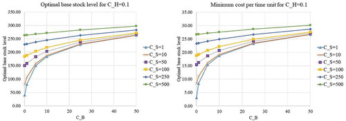
Figure B2. Optimal base stock level and minimum cost per time unit for $C_H$= 1.

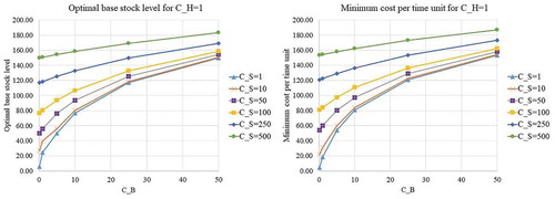
Figure B3. Optimal base stock level and minimum cost per time unit for $C_H$= 5.

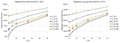
Figure B4. Optimal base stock level and minimum cost per time unit for $C_H$= 10.

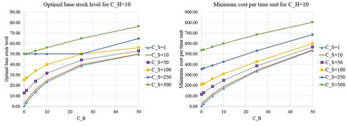
Figure B5. Optimal base stock level and minimum cost per time unit for $C_H$= 25.

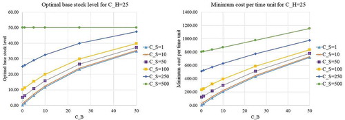
Figure B6. Optimal base stock level and minimum cost per time unit for $C_H$= 50.

References

- Atasoy, B., Güllü, R., & Tan, T. (2012). Optimal inventory policies with non-stationary supply disruptions and advance supply information. Decision Support Systems, 53(2), 269–27. https://doi.org/10.1016/j.dss.2012.01.005
- Axsäter, S. (2015). Inventory Control. Springer, New York. https://doi.org/10.1007/978-3-642-48417-9_158
- Bakal, İ. S., Bayındır, Z. P., & Emer, D. E. (2017). Value of disruption information in an EOQ environment. European Journal of Operational Research, 263(2), 446–460. https://doi.org/10.1016/j.ejor.2017.04.045
- Berk, E., & Arreola‐Risa, A. (1994). Note on “Future supply uncertainty in EOQ models”. Naval Research Logistics, 41(1), 129–132. https://doi.org/10.1002/1520-6750(199402)41:1<129::aid-nav3220410109>3.0.co;2-m
- Ciarallo, F. W., & Niranjan, S. (2014). Properties of optimal order-up-to levels for the newsvendor problem with random capacity. International Journal of Advanced Operations Management, 6(4), 353–376. https://doi.org/10.1504/ijaom.2014.066830
- de Kok, T., & Graves, S. (2003). Handbooks in operations research and management science: Supply chain management. https://doi.org/10.1016/s0927-0507(00)x0002-3
- De, S. K., & Mahata, G. C. (2020). A production inventory supply chain model with partial backordering and disruption under triangular linguistic dense fuzzy lock set approach. Soft Computing, 24(7), 5053–5069. https://doi.org/10.1007/s00500-019-04254-2
- Fathalizadeh, S., Mirzazadeh, A., & Ghodratnama, A. (2019). Fuzzy inventory models with partial backordering for deteriorating items under stochastic inflationary conditions: Comparative comparison of the modeling methods. Cogent Engineering, 6(1), 1648630. https://doi.org/10.1080/23311916.2019.1648630
- Firouzi, F., Baglieri, E., & Jaber, M. Y. (2014). Two-product inventory management with fixed costs and supply uncertainty. Applied Mathematical Modelling, 38(23), 5635–5650. https://doi.org/10.1016/j.apm.2014.03.018
- Greising, D., & Johnsson, J., (2007 December 8). Behind Boeing 787 delays: Problems at one of the smallest suppliers in Dreamliner program causing ripple effect. Chicago Tribune [online]. Accessed March 1, 2019. http://articles.chicagotribune.com/2007-12-08/news/0712070870_1_dreamliner-boeing-spokeswoman-suppliers
- Güllü, R., Önol, E., & Erkip, N. (1999). Analysis of an inventory system under supply uncertainty. International Journal of Production Economics, 59(1–3), 377–385. https://doi.org/10.1016/s0925-5273(98)00024-3
- Heimann, D., & Waage, F. (2007). A closed-form approximation solution for an inventory model with supply disruptions and non-ZIO reorder policy. Journal of Systemics. Cybernetics and Informatics, 5(4), 1–12.
- Hsieh, C. C., & Putera, R. R. (2018). Mitigating supply disruption with ordering and supply restoration decisions. Computers & Industrial Engineering, 126, 681–690. https://doi.org/10.1016/j.cie.2018.10.025
- Jauhari, W. A., Mayangsari, S., Kurdhi, N. A., & Wong, K. Y. (2017). A fuzzy periodic review integrated inventory model involving stochastic demand, imperfect production process and inspection errors. Cogent Engineering, 4(1), 1308653. https://doi.org/10.1080/23311916.2017.1308653
- Jauhari, W. A., & Saga, R. S. (2017). A stochastic periodic review inventory model for vendor–buyer system with setup cost reduction and service–level constraint. Production & Manufacturing Research, 5(1), 371–389. https://doi.org/10.1080/21693277.2017.1401965
- Konstantaras, I., Skouri, K., & Lagodimos, A. G. (2019). EOQ with independent endogenous supply disruptions. Omega, 83, 96–106. https://doi.org/10.1016/j.omega.2018.02.006
- Lewis, B. M., Erera, A. L., Nowak, M. A., & Chelsea, C. W., III. (2013). Managing inventory in global supply chains facing port-of-entry disruption risks. Transportation Science, 47(2), 162–180. https://doi.org/10.1287/trsc.1120.0406
- Li, Z., Xu, S. H., & Hayya, J. (2004). A periodic-review inventory system with supply interruptions. Probability in the Engineering and Informational Sciences, 18(1), 33–53. https://doi.org/10.1017/s0269964804181035
- Lücker, F., Seifert, R. W., & Biçer, I. (2019). Roles of inventory and reserve capacity in mitigating supply chain disruption risk. International Journal of Production Research, 57(4), 1238–1249. https://doi.org/10.1080/00207543.2018.1504173
- Mohebbi, E. (2003). Supply interruptions in a lost-sales inventory system with random lead time. Computers & Operations Research, 30(3), 411–426. https://doi.org/10.1016/s0305-0548(01)00108-3
- Mohebbi, E. (2004). A replenishment model for the supply-uncertainty problem. International Journal of Production Economics, 87(1), 25–37. https://doi.org/10.1016/s0925-5273(03)00098-7
- Norrman, A., & Jansson, U. (2004). Ericsson’s proactive supply chain risk management approach after a serious sub-supplier accident. International Journal of Physical Distribution and Logistics Management, 34(5), 434–456. https://doi.org/10.1108/09600030410545463
- Orgeldinger, J. (2018). Recent issues in the implementation of the new basel minimum capital requirements for market risk. Emerging Science Journal, 2(2), 65–77. https://doi.org/10.28991/esj-2018-01129
- Parlar, M., & Berkin, D. (1991). Future supply uncertainty in EOQ models. Naval Research Logistics, 38(1), 107–121. https://doi.org/10.1002/1520-6750(199102)38:1<107::aid-nav3220380110>3.0.co;2-4
- Parlar, M., & Perry, D. (1996). Inventory models of future supply uncertainty with single and multiple suppliers. Naval Research Logistics, 43(2), 191–210. https://doi.org/10.1002/(sici)1520-6750(199603)43:2<191::aid-nav3>3.0.co;2-5
- Parlar, M., Wang, Y., & Gerchak, Y. (1995). A periodic review inventory model with Markovian supply availability. International Journal of Production Economics, 42(2), 131–136. https://doi.org/10.1016/0925-5273(95)00115-8
- Prahalad, C. K., & Hamel, G. (1990). The core competence of the corporation. Harvard Business Review, 68, 79–91.
- Qi, L., Shen, Z. J. M., & Snyder, L. V. (2009). A continuous‐review inventory model with disruptions at both supplier and retailer. Production and Operations Management, 18(5), 516–532. https://doi.org/10.1111/j.1937-5956.2009.01026.x
- Ross, S. M. (1996). Stochastic Processes (2nd ed.). Wiley.
- Saga, R. S., Jauhari, W. A., Laksono, P. W., & Dwicahyani, A. R. (2019). Investigating carbon emissions in a production-inventory model under imperfect production, inspection errors and service-level constraint. International Journal of Logistics Systems and Management, 34(1), 29–55. https://doi.org/10.1504/ijlsm.2019.102062
- Saithong, C., & Luong, H. T. (2019). Effect of supply disruption on inventory policy. European Journal of Industrial Engineering, 13(2), 178–212. https://doi.org/10.1504/ejie.2019.10020067
- Saithong, C., & Luong, H. T. (in press). Effects of supply disruption on optimal inventory policy: The case of (r,S) continuous review inventory policy. International Journal of Industrial and Systems Engineering. https://doi.org/10.1504/ijise.2020.10020418
- Salehi, H., Taleizadeh, A. A., & Tavakkoli-Moghaddam, R. (2016). An EOQ model with random disruption and partial backordering. International Journal of Production Research, 54(9), 2600–2609. https://doi.org/10.1080/00207543.2015.1110634
- Schmitt, A. J., & Snyder, L. V. (2012). Infinite-horizon models for inventory control under yield uncertainty and disruptions. Computers & Operations Research, 39(4), 850–862. https://doi.org/10.1016/j.cor.2010.08.004
- Schmitt, A. J., Snyder, L. V., & Shen, Z. J. M. (2010). Inventory systems with stochastic demand and supply: Properties and approximations. European Journal of Operational Research, 206(2), 313–328. https://doi.org/10.1016/j.cor.2010.08.004
- Sevgen, A., & Sargut, F. Z. (2019). May reorder point help under disruptions? International Journal of Production Economics, 209, 61–69. https://doi.org/10.1016/j.ijpe.2018.02.014
- Shahbaz, M. S., Soomro, M. A., Bhatti, N. U. K., Soomro, Z., & Jamali, M. Z. (2019). The impact of supply chain capabilities on logistic efficiency for the construction projects. Civil Engineering Journal, 5(6), 1249–1256. https://doi.org/10.28991/cej-2019-03091329
- Skouri, K., Konstantaras, I., Lagodimos, A. G., & Papachristos, S. (2014). An EOQ model with backorders and rejection of defective supply batches. International Journal of Production Economics, 155, 148–154. https://doi.org/10.1016/j.ijpe.2013.11.017
- Snyder, L. V. (2014). A tight approximation for an EOQ model with supply disruptions. International Journal of Production Economics, 155, 91–108. https://doi.org/10.1016/j.ijpe.2014.01.025
- Spilbergs, A. (2020). Residential mortgage loans delinquencies analysis and risk drivers assessment. Emerging Science Journal, 4(2), 104–112. https://doi.org/10.28991/esj-2020-01214
- Taleizadeh, A. A. (2017). Lot‐sizing model with advance payment pricing and disruption in supply under planned partial backordering. International Transactions in Operational Research, 24(4), 783–800. https://doi.org/10.1111/itor.12297
- Taleizadeh, A. A., & Dehkordi, N. Z. (2017). Economic order quantity with partial backordering and sampling inspection. Journal of Industrial Engineering International, 13(3), 331–345. https://doi.org/10.1007/s40092-017-0188-8
- Tomlin, B. (2006). On the value of mitigation and contingency strategies for managing supply chain disruption risks. Management Science, 52(5), 639–657. https://doi.org/10.1287/mnsc.1060.0515
- Warsing, D. P., Jr, Wangwatcharakul, W., & King, R. E. (2013). Computing optimal base-stock levels for an inventory system with imperfect supply. Computers & Operations Research, 40(11), 2786–2800. https://doi.org/10.1016/j.cor.2013.04.001
- Zhang, S., Zhang, P., & Zhang, M. (2019). Fuzzy emergency model and robust emergency strategy of supply chain system under random supply disruptions. Complexity, 3092514. https://doi.org/10.1155/2019/3092514