Sensitivity analysis of a single phase to ground fault system in connection with high impedance faults: A case study

Abstract

Most of High-impedance faults (HIFs) occur due to broken conductors falling on high-resistivity desert soil in United Arab Emirates remain undetected due to incredibly low fault currents and endanger lives. A reliable detection method is needed. A live line test conducted on a 11kV distribution line by switching to a remotely laid conductor did not result enough detectable fault currents. This motivated conducting a literature survey and researching for the reasons why the modern numerical protection relays could not detect such low current faults. Hence, a sensitivity analysis of a single-phase-to-ground system is carried out. Mathematical modelling for the sensitivity analysis is performed using differential calculus. Applying definition of sensitivity to a set of power system equations to analyze to provide guidance for detection of high impedance faults is entirely a new approach. This paper provides a comprehensive analysis of single phase to ground fault system by exhibiting profiles of fault currents, line, neutral, and MV bus voltages for a range of fault impedance. The sensitivity analysis results conclude that low-fault current signals should be collected from the neutral line of the distribution system instead of focusing on the line voltage, current, power and other parameters.

Keywords:

• Bus voltages
• calculus
• desert soil resistivity
• fallen conductor
• line voltages
• neutral current and voltage
• profiles of primary currents and voltages
• real system data
• symmetrical components
• sensitivity analysis
• sequence impedances
• zero sequence current

PUBLIC INTEREST STATEMENT

High-impedance faults (HIFs) often occur due to broken conductors falling on high-resistivity desert soil. To understand the characteristics and magnitude of the current produced by the fallen conductors in the desert, under different situations, 11 kV live line fault simulations in desert region were conducted by power supply providers. The author⁽¹⁾, who was involved as a lead engineer (competent person) in conducting such tests, analyzed the power system to identify methods to measure such low fault currents. Therefore, authors viewed it from power system point of view to carry out sensitivity analysis and to analyze the degree of severity of high impedance faults. The main motivation is to detect high impedance faults due to fallen conductor in desert soil and thereby to ensure humans and animals safety in desert region.

1. Introduction

High-impedance faults (HIFs) frequently occur in the Middle East region due to fallen broken conductors in overhead lines. Such faults remain undetected due to low- or very-low-fault currents. A literature survey is undertaken to understand in this area and the summary is included.

The IEEE power system relaying committee working group D15 (PSRC WGD15) report (Tengdin et al., 1996) stated that HIFs on the distribution system created a unique challenge for protection engineers. This was a status report in 1996. A much earlier IEEE Power Engineering Society (PES) publication (IEEE Power Engineering Society, Downed Power Lines, 1989) from 1989 explained why downed conductors in electric power lines could not always be detected.

The PSRC WGD15 report (Tengdin et al., 1996) covered work since 1970 and reported that high impedance faults (HIFs) on distribution systems create unique challenges for protection engineers. HIFs do not produce enough fault current to be detectable by conventional overcurrent relays or fuses. New detectors should be capable of providing a new tool that can help minimize the public’s exposure to downed conductors. The EPRI and CEA directed research that resulted in several research reports (Balser et al., 1982; Carr & Hood, 1979; Lee, 1982; Russell et al., 1982) on HIFs.

Since then, researchers have studied and applied many existing and emerging techniques to HIF detection. These include statistical hypothesis tests (Balser et al., 1986), inductive reasoning and expert systems (Kim & Russell, 1989), a third harmonic phase angle of fault currents (Jeerings & Linders, 1991), Neural networks (NNs) (Apostolov et al., 1993; Ebron et al., 1990), wavelet decomposition (Apostolov et al., 1993; Lai et al., 2006), decision trees (Sheng & Rovnyak, 2004), decision fuzzy logic (Jota & Jota, 1998), a combination of wavelet transformation (WT) and NNs (Yang et al., 2004), A real-coded genetic algorithm (RCGA) to analyze the harmonic and phase angle of HIF currents (Zamanan, 2007), evaluation of zero- and negative-sequence currents with real networks (Louro & De Sa, 2007), and PSCAD/EMTDC software-simulated analysis for various single-phase fault types with a “phase discontinuity” protective function (Papathanassiou et al., 2007).

A new HIF detection system applying the “multi-algorithm” approach and results from laboratory tests (Das & Bayoumi, 2007) was conducted. The research continued. A theoretical study simulation, laboratory tests and an analysis of field test recordings (Masa et al., 2011) were carried out. An alternative transient programme/electromagnetic transient programme (ATP/EMTP) model of HIFs was developed and simulated to understand the effect of an arc in a HIF. However, not all characteristics of HIFs could be studied by simulation. HIF detection using a digital signal processor (DSP) to design a system that could detect unwanted and dangerous frequencies (Boudjit et al., 2012) by eliminating the main frequency with a finite impulse response (FIR) filter was discussed. The detection of low-current faults (LCFs) produced by high-resistance faults was addressed by using an LCF detection algorithm (Zamora et al., 2012) for the high-impedance grounded system discussed. Validation of the algorithm (Zamora et al., 2002) was attempted by using the software RESFAL, programmed in the MATLAB/SIMULINK environment.

Various HIF detection methods and fault location techniques were reviewed and compared to highlight future work (Ghaderi & Mohammadpour, 2017) in a single paper for the period 1982–2015. In this paper, the HIF detection techniques are categorized, evaluated, and compared with one another by referring to a total of 210 literatures. The real-time detection of transients induced by HIFs based on the boundary wavelet transform (WT) was discussed (Costa et al., 2015); however, the simulated data assumed a current signal at a level of approximately 35 A over 40 cycles, which can be easily detected by numerical relays. High-sensitivity vegetation HIF detection based on a signal’s high-frequency contents was discussed (Gomes et al., 2018), and future investigations will have to address the hardware implementation possibilities. The application of smart meters in HIF detection on distribution systems was discussed (Chakraborty & Das, 2018), and the proposed method was based on voltage sag-swell, capacitor/load switching, transformer energization, feeder energization, power electronic loads, arc furnace loads, and distributed generators (DGs). The performance of the proposed method was evaluated using both PSCAD simulations and an experimental setup. Real-time data were not derived or used. A feature selection method for HIF detection was discussed (Cui et al., 2019); however, no physical experiment was performed to prove the detection capability of such a method. A negative selection algorithm (NSA)-based identification framework for distribution network faults with high resistance was proposed (Song et al., 2019); however, a simulation system was made using MATLAB/SIMULINK and not in a real-time environment.

Based on the above literature survey, one of the main noteworthy points is that the published methods and simulations primarily utilize signals that are not real-time signals. Instead, the signals are derived from software signal generators. Hence, these methods demonstrate higher sensitivity and reliability than methods based on real-time signals. This means that analysis based on real system data and a practical model to derive suitable signals is required. Thus, the detection of HIFs has been one of the most persistent and difficult problems faced by electric power distribution companies that continue to explore means to detect such faults.

In this paper, sensitivity analysis using differential calculus is performed based on real system data by computing fault currents and voltages for a range of fault impedances and choosing different values of neutral impedance. Sensitivity analysis is performed by the authors to analyze the degree of severity of HIFs, and we consider it as a design tool to improve the value of the neutral impedance by observing voltages in healthy and neutral phases. Based on the literature survey provided, we are not able to compare those engineering results with the results of our work, which are entirely new and done first time.

The sensitivity analysis is important for any system when it is considered as a multivariable system. The concept of sensitivity is basically a control system concept and it is very closely related to tuning of a parameter to achieve a certain value of an objective function or output. However, when we focus on a power system, the above said objective function becomes “fault current” and there exists so many parameters once the expression for fault current in a single line to ground fault is observed minutely. If the fault current in a single line to ground fault in a power system is taken as main objective function, it can be observed from the fault current equation that there are a couple of parameters which can be tuned either off-line (design) problem or on-line problem. If this problem is taken as an off-line problem (design) problem, then each of sequence impedances (Z₁, Z₂, Z₀) and the neutral impedance (Z_n) can be fixed on a trial basis to control the fault current. When it is a problem of detection of high impedance fault in the field (this is what our paper targets), then fault impedance or neutral impedance appears as of prior importance for tuning the system. Contributions of this work are mainly to;

• Provide a comprehensive analysis of single phase to ground fault system by exhibiting profiles of fault currents, line, neutral and MV bus voltages for a range of fault impedance.

• Apply definition of sensitivity to a set of power system equations to analyze and provide guidance for detection of high impedance faults by conducting a case study for medium voltage distribution line in desert region.

Furthermore, the sensitivity analysis can be extended to isolated power systems using dedicated generators (application of such generators by itself can be a future study) to feed to desert regions, and in this case the sensitivity analysis could point to tuning more parameters such as reactances of generator in addition to tuning neutral earthing impedance. This sensitivity analysis can also be extended to include the line charging capacitances and its effect.

The rest of this paper is divided into eight sections. Section 2 provides a single line diagram representation of a typical three-phase distribution system and includes electrical data of real system in a desert region. Section 3 highlights the importance of understanding the neutral current and neutral voltage with respect to the zero-potential line and explains the current and voltage transformation ratios in relation to the sensitivity analysis. Section 4 includes current and voltage calculations for a single-phase-to-ground fault for a real system for a range of fault impedances at a fault location “F” and for chosen values of neutral impedance. Live-line test results are included and compared with the calculated results. In Section 5, the correctness of the complete range of calculated results using a spreadsheet is validated using proven commercial software for two sample cases. In Section 6, mathematical modelling and sensitivity calculations for fault current and voltages are detailed. Section 7 is used to present the case of fallen-conductor contact resistance on desert soil in support of the fault-impedance range chosen in the analysis. Conclusions are given in Section 8.

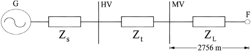
2. Representation of a typical distribution system in desert region

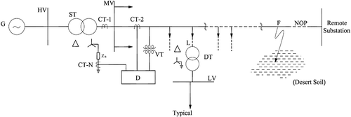
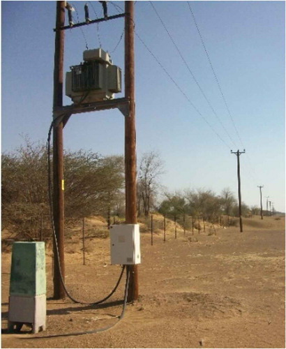
A typical three-phase distribution system and a single-phase-to-ground fault “F” on a desert soil are represented in Figure 1. The distribution system’s real data and a picture of a wooden pole overhead line together with pole mounted DT (distribution transformer) in desert region are shown respectively in Table 1 and Figure 2.

Table 1. Real system data

Real System Data
System Voltage	: 33 kV
3-Phase Fault	: 1636.7 MVA
1-Phase Fault	: 571.56 MVA
Station Transformer Data
Rating	: 20 MVA
Voltage	: 33/11 kV
Current	: 349.9/1049.7 A
Impedance	: 12% at 20 MVA base
Neutral Earthing impedance	: 0.1 Ω ^1: 25.4, 63.5, 254 and 635 Ω ^2
Distribution Transformer Data
Rating	: 0.5 MVA or 1 MVA
Voltage	: 11/0.4 kV
Overhead line (OHL)
Construction	: Wooden pole, (Al) conductor, no ground wire (refer Figure 2)
Conductor cross section area	: 70 Sq.mm
Length ^3	: 2756 m

¹Solid grounding in real system.

²Analysis considers neutral earthing resistors. Each value chosen is a fraction of 6350 which is the value of phase to neutral voltage.

³Live line test conducted at this location (Velmurugan, 2012).

Figure 1. Single-line diagram.

The sensitivity analysis requires understanding of (a) basic concepts of neutral voltage of a three phase system (b) practical transformation ratios of instrument transformers used for measurement of voltages and currents and (c) effects of such transformation ration in the sensitivity analysis and the parameters involved in such analysis. Hence, a Section 3 is devoted in bringing out related information for ready reference.

Figure 2. Wooden pole overhead line & pole mounted (11/0.4 kV) DT distribution transformer in desert region.

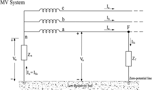
3. Representation of neutral current and voltage

The neutral line of a three-phase system is connected to the ground directly or through grounding impedances. Figure 3 shows a line-to-ground fault at “F” through fault impedance “Z_f”. It is important, in this analysis, to understand the voltage across the neutral line of a three-phase system, the voltages “V_n” and “V_an” are defined by the following equation for phase “a”:

(1) $V_{an}=V_a-V_n=V_a+I_n{Z}_n$(1)

Figure 3. Representation of neutral current and voltage.

In real-time measurements, instrument transformers are used to measure and analyze the primary voltages and currents safely. A current transformation ratio of 300/1 or 400/1 and a voltage transformation ratio of 11,000/110 are used in a medium-voltage distribution system. The neutral current transformation ratio of the station transformer (ST) is 1200/1 for a solidly earthed system. In the case of a high resistance/impedance grounded system, a current transformation of 30/1 or lower is used. Such a low transformation ratio is essential in the detection of low zero-sequence current produced by high impedance faults. The transformation of the primary-fault impedance “Z_f” to secondary-fault impedance is calculated using the CT ratio and VT ratio. Later in this paper, the sensitivity of fault current to fault impedance is discussed. The sensitivity is a ratio and has no units. Therefore, CT and VT ratios do not affect the results of the sensitivity analysis.

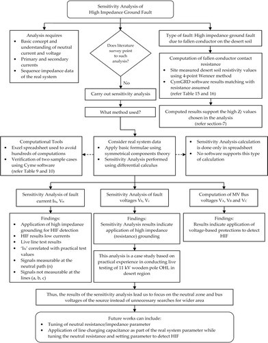
To understand the method involved in the computation of sensitivity analysis of high impedance ground fault, a flow chart is given in Figure 4. The organization of the flow chart is made in such a way that it reflects the body of the entire paper presented and helpful while reading through different many sections containing considerable technical information and computational results.

Figure 4. Flowchart for sensitivity analysis of high impedance ground fault.

4. Calculation of the fault current and voltages

It is assumed that fault impedance is entirely resistive in nature. The reactive part of the fault impedance in desert soil is insignificant and hence can be neglected. Additionally, resistance-neutral grounding is assumed in the calculation, although the word “impedance” is used throughout this paper. The profiles of voltages and currents are plotted with enough information for the reader to understand without the need for explanation. Presenting information in tabular form is minimized.

For the purpose of calculation of fault current and voltages, a simplified single-line diagram of the distribution system showing the bus names and impedances is given in Figure 5.

Figure 5. Simplified single-line diagram.

The sequence impedance data of the real system is given below in Table 2.

Table 2. Sequence impedance data of the real system

Source Impedance (ZS)—referred in 11 kV
Positive seq. impedance (Z1 S)	: 0.0689 + j0.662 Ω
Negative seq. impedance (Z2 S)	: 0.0689 + j0.662 Ω
Zero seq. impedance (Z0 S)	: 0.4543 + j4.362 Ω
Transformer Impedance (Zt)
Positive seq. impedance (Z1 t)	: 0.0287 + j0.7254 Ω
Negative seq. impedance (Z2 t)	: 0.0287 + j0.7254 Ω
Zero seq. impedance (Z0 t)	: 0.0287 + j0.6892 Ω
Neutral Earthing impedance (Zn)	: 0.1 + j0 Ω
Zero seq. impedance of neutral earthing (3Zn)	: 0.3 + j0 Ω
Zero seq. impedance (Z0 t + 3Zn)	: 0.3287 + j0.689 Ω
Impedance (ZL)
Positive seq. impedance (Z1 L)	: 0.9335 + j0.9787 Ω
Negative seq. impedance (Z2 L)	: 0.9335 + j0.9787 Ω
Zero seq. impedance (Z0 L)	: 1.342 + j4.465 Ω
Total Sequence Impedances
Z1- Positive seq. impedance (Z1 S + Z1 t + Z1 L)	: 0.969 + j1.778 Ω
Z2- Negative seq. impedance (Z2 S + Z2 t + Z2 L)	: 0.969 + j1.778 Ω
Z0- Zero seq. impedance (Z0 L + Z0 t + 3Zn)	: 1.671 + j5.154 Ω
Let fault impedance (Zf) be	: 35.45 Ω

4.1. Calculation for I_fa

The following well-known formula (Grainger & Stevenson, 1994) based on symmetrical components is used for computing the single-phase-to-ground fault current “I_fa” at “F”:

(2) $I_{fa}=3I_{a0}=\frac{V_a}{\left(Z_1+Z_2+Z_0+3Z_n+3Z_f\right)}$(2)

The single-phase-to-ground fault current “I_fa” is calculated using Eq. (2)(2) $I_{fa}=3I_{a0}=\frac{V_a}{\left(Z_1+Z_2+Z_0+3Z_n+3Z_f\right)}$(2) substituting relevant data from Table 2:

$I_{fa}=172.7\mathrm{\angle }-{4.7}^{\circ }A$.

Similarly, the fault current “I_fa” for various fault impedances (0.1–1000 ohms) is calculated considering different neutral grounding impedances (0.1, 25.4, 63.5, 254 and 635 ohms), and the results are tabulated and plotted.

It can be seen from Figure 6 that the fault current does not vary significantly in the case of high “Z_n” (for example, 635 ohms) for the chosen range of fault impedance values (0.1–1000 ohms). This clearly suggests the application of low or very low CT ratios in neutral circuits with high “Z_n” values. A CT ratio of 10/1 can be employed to detect very low fault currents when “Z_n” is 635 ohms (refer to Table 3).

Figure 6. Magnitude of calculated fault current (I_fa) for Z_f = 0.1 to 1000 Ω for different “Z_n”. Graph is drawn omitting “θ” (key values are in Table 3).

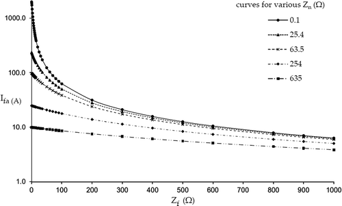
Table 3. Calculated fault currents for different neutral earthing and fault impedances

Zf (Ω)	Zn (Ω)
	0.1	25.4	63.5	254	635
	Fault current Ifa (A)
0.1	1995.62	237.31	98.05	24.88	9.98
10	548.74	173.43	85.06	23.95	9.83
30	202.66	112.25	67.10	22.27	9.53
35.45	172.73	102.40	63.45	21.86	9.46
100	62.73	50.19	38.58	17.88	8.63
500	12.67	12.06	11.25	8.41	5.59
1000	6.34	6.19	5.97	5.06	3.88

Live line test results on a 11kV wooden pole line in desert region are given here for three cases, (case-1) fault simulation by switching on to a bolted connection to ground via the pole mounted (11/0.4kV) transformer grounding connections and (case-2 and case-3) by switching on the live line to an already laid conductor (simulation of a fallen conductor) on the ground. The station transformer neutral is solidly earthed during fault simulations.

• Case-1: The fault current (I_N = 173 A) is a measured value in a live line test conducted (2014) in a neutral solidly earthed system with Z_n = 0.1 ohms. A bolted fault at a distribution transformer (DT) at a distance of 2756 m is made, and the calculated fault impedance is 35.45 ohms. The fault current is limited due to high resistive soil and no return of fault current due to wooden pole OHL having no earth wire. The measured voltage and current waveforms and their magnitudes are shown in Figure 7 and Table 4, respectively. The author⁽¹⁾ was involved as a lead engineer (competent person) in conducting these tests (Velmurugan, 2012).

• Case-2: 4.9A fault current for a single phase to ground fault to a fallen conductor indicating high impedance fault. The resulting fault impedance is about 1300 Ohms. The measured voltage and current waveforms and their magnitudes are shown in Figure 8 and Table 4, respectively.

• Case-3: 0.368A fault current for a single phase to ground fault to a fallen conductor. The resulting fault impedance is about 17 K Ohms. The measured bus voltage and current waveforms and their magnitudes are shown in Figure 9 and Table 4, respectively.

Figure 7. Recorded voltage and current waveforms for case—1. (Field-measured values are in Table 4).

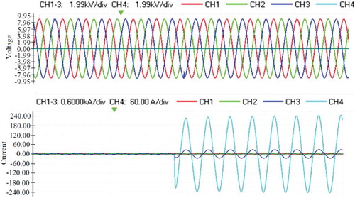
Figure 8. Recorded voltage and current waveforms for case—2. (Field-measured values are in Table 4).

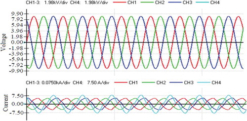
Figure 9. Recorded voltage and current waveforms for case—3. (Field-measured values are in Table 4).

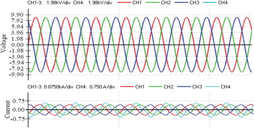
Table 4. Field measured values for case—1, 2 and 3

Bus voltages	Case-1	Case-2	Case-3	Phase currents	Case-1	Case-2	Case-3
	Voltage (CH1-3, CH4) (kV)				Current (CH1-3, CH4) (A)
VA	6.324	6.414	6.400	IA	191.8	34.9	29.4
VB	6.330	6.388	6.381	IB	39.5	34.4	30.3
VC	6.351	6.407	6.400	IC	44.0	34.9	29.7
VN	0.017	0.000	0.000	IN	173.0	4.9	0.368

Natures of low current waveform indicate “arcing” in the soil during the fault current. Due to arcing, the soil gets heated up and the high resistance formed due to arcing extinguishes the fault, resulting fault current eventually to zero.

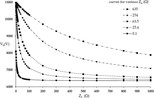
4.2. Calculation of line voltages V_b and V_c

The healthy line voltage of phase “b” (Kothari & Nagrath, 2007) is, as an example, calculated using Equation (3)(3) $V_b=\frac{V_a\left(3{\alpha }^2{Z}_f+Z_2\left({\alpha }^2-\alpha \right)+(Z_0+3Z_n)\left({\alpha }^2-1\right)\right)}{\left(Z_1+Z_2+Z_0+3Z_n+3Z_f\right)}$(3) substituting relevant data from Table 2:

(3) $V_b=\frac{V_a\left(3{\alpha }^2{Z}_f+Z_2\left({\alpha }^2-\alpha \right)+(Z_0+3Z_n)\left({\alpha }^2-1\right)\right)}{\left(Z_1+Z_2+Z_0+3Z_n+3Z_f\right)}$(3)

$V_b=6544V$.

Figure 10. Magnitude of the line voltage (V_b) for Z_f = 0.1 to 1000 Ω for different Z_n values. Graph is drawn omitting “θ”.

The healthy line voltage of phase “c” (Kothari & Nagrath) is, as an example, calculated using Eq. (4)(4) $V_c=\frac{V_a\left(3\alpha Z_f+Z_2\left(\alpha -{\alpha }^2\right)+(Z_0+3Z_n)\left(\alpha -1\right)\right)}{\left(Z_1+Z_2+Z_0+3Z_n+3Z_f\right)}$(4) substituting relevant data from Table 2:

(4) $V_c=\frac{V_a\left(3\alpha Z_f+Z_2\left(\alpha -{\alpha }^2\right)+(Z_0+3Z_n)\left(\alpha -1\right)\right)}{\left(Z_1+Z_2+Z_0+3Z_n+3Z_f\right)}$(4)

$V_C=6215.2V$.

Figure 11. Magnitude of the line voltage (V_c) for Z_f = 0.1 to 1000 Ω for different Z_n values. Graph is drawn omitting “θ”.

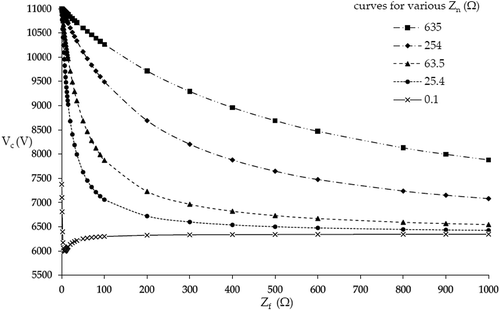
For various values of “Z_n”, the profiles of healthy line voltages “V_b” and “V_c” in Figures 10 and 11, respectively, indicate (i) that the voltages are limited appropriately in the case of solid neutral grounding and (ii) over-voltages occur in the case of resistance grounding (Kothari & Nagrath). The magnitude of the over-voltage decreases as the fault impedance increases. It is important from the safety viewpoint that limiting over-voltages is not a vital goal when such information in the system can be used for the detection of faults.

4.3. Calculation for the MV Bus Voltages V_A, V_B and V_C

The MV bus voltages are calculated based on relevant data from Table 2 by appropriately using Eqs. (3)(3) $V_b=\frac{V_a\left(3{\alpha }^2{Z}_f+Z_2\left({\alpha }^2-\alpha \right)+(Z_0+3Z_n)\left({\alpha }^2-1\right)\right)}{\left(Z_1+Z_2+Z_0+3Z_n+3Z_f\right)}$(3) and (4(4) $V_c=\frac{V_a\left(3\alpha Z_f+Z_2\left(\alpha -{\alpha }^2\right)+(Z_0+3Z_n)\left(\alpha -1\right)\right)}{\left(Z_1+Z_2+Z_0+3Z_n+3Z_f\right)}$(4) ) for a fault “F” for various “Z_f” values (0.1–1000 ohms) and for various “Z_n” values to plot the profiles of voltages V_A, V_B, and V_C at the MV bus. The equations for calculating MV bus voltages are not included here, only voltage profiles are given to exhibit the voltage variation with respect to “Z_f” and “Z_n”. Refer Section 5 for validation of complete results presented here.

Figure 12. Magnitude of the MV bus voltage (V_A) for Z_f = 0.1 to 1000 Ω for different “Z_n” values. Graph is drawn omitting “θ” (key values are in Table 5).

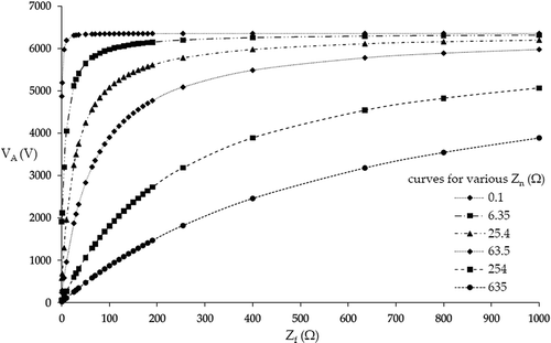
Figure 13. Magnitude of the MV bus voltage (V_B) for Z_f = 0.1 to 1000 Ω for different “Z_n” values. Graph is drawn omitting “θ” (key values are in Table 6).

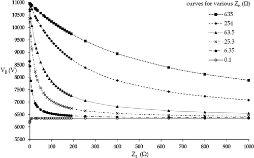
Figure 14. Magnitude of the MV bus voltage (V_C) for Z_f = 0.1 to 1000 Ω for different “Z_n” values. Graph is drawn omitting “θ” (key values are in Table 7).

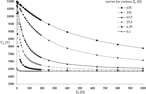
Table 5. Magnitude of MV Bus voltage (V_A) for various fault impedances

Zf (Ω)	Zn (Ω)
	0.1	6.35	25.4	63.5	254	635
	MV Bus voltage VA (kV)
0.1	4.87	1.91	0.58	0.24	0.06	0.02
10	6.19	4.05	1.96	0.96	0.27	0.11
30	6.31	5.27	3.50	2.09	0.69	0.30
35.45	6.32	5.40	3.75	2.32	0.80	0.35
100	6.34	5.97	5.07	3.90	1.81	0.87
400	6.35	6.25	5.97	5.48	3.89	2.46
1000	6.35	6.31	6.19	5.97	5.07	3.89

Table 6. Magnitude of MV Bus voltage (V_B) for various fault impedances

Zf (Ω)	Zn (Ω)
	0.1	6.35	25.4	63.5	254	635
	MV Bus voltage VB (kV)
0.1	6.18	8.64	10.36	10.75	10.94	10.97
10	6.35	7.45	9.15	10.07	10.74	10.89
30	6.35	6.88	8.06	9.17	10.37	10.73
35.45	6.35	6.81	7.89	8.99	10.29	10.69
100	6.35	6.54	7.05	7.84	9.46	10.24
400	6.35	6.40	6.55	6.82	7.87	8.95
1000	6.35	6.37	6.43	6.55	7.08	7.87

Table 7. Magnitude of MV Bus voltage (V_C) for various fault impedances

Zf (Ω)	Zn (Ω)
	0.1	6.35	25.4	63.5	254	635
	MV Bus voltage VC (kV)
0.1	6.54	10.70	11.04	11.03	11.01	11.00
10	6.40	8.00	9.57	10.30	10.80	10.92
30	6.37	7.02	8.26	9.33	10.44	10.76
35.45	6.37	6.92	8.06	9.14	10.35	10.72
100	6.36	6.56	7.10	7.90	9.50	10.27
400	6.35	6.40	6.55	6.83	7.88	8.96
1000	6.35	6.37	6.43	6.55	7.08	7.88

Graphical plots for MV voltages V_A, V_B, and V_C are shown in Figures 12–14, respectively. These voltages can be monitored by voltage transformers and relay circuits at the MV bus. However, the line voltages “V_b” and “V_c” shown in Figures 10 and 11, respectively, for any fault on the line are obviously not measurable. The MV voltage profiles for solidly grounded system with low impedance faults show the known fact that the MV bus voltages are closer to operating voltage of 6350 V. This limited discussion is considered as sufficient.

4.4. Transformer neutral voltage V_N

The neutral voltage increases for higher values of “Z_n”, as shown in Figure 15.

Figure 15. Magnitude of neutral voltage (V_N) for Z_f = 0.1 to 1000 Ω for different “Z_n” . Graph is drawn omitting “θ” (key values are in Table 8).

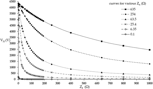
Table 8. Magnitude of neutral voltage (V_N) for various fault impedances

Zf (Ω)	Zn (Ω)
	0.1	6.35	25.4	63.5	254	635
	Neutral voltage VN (kV)
0.1	0.199	4.98	6.03	6.23	6.32	6.34
10	0.055	2.28	4.41	5.40	6.08	6.24
30	0.020	1.07	2.85	4.26	5.66	6.05
35.45	0.017	0.94	2.60	4.03	5.55	6.01
100	0.006	0.38	1.27	2.45	4.54	5.48
400	0.001	0.09	0.38	0.87	2.46	3.89
1000	0.001	0.04	0.16	0.38	1.29	2.46

The magnitude of over-voltage decreases as the fault impedance increases. In desert regions, fault impedances are generally high (based on practical experience in conducting live line tests for a “bolted” ground fault at the fault location “F”, the fault impedance “Z_f” is higher by approximately 35.45 ohms on a wooden pole DT). A multistage over-voltage protection relay can be employed to detect ground faults in the case of a neutral resistor-grounded neutral system.

5. Software computation of the fault voltages V_A, V_B and V_C

To validate the correctness of the complete range of calculated results presented here using a spreadsheet for solving Eqs. (3)(3) $V_b=\frac{V_a\left(3{\alpha }^2{Z}_f+Z_2\left({\alpha }^2-\alpha \right)+(Z_0+3Z_n)\left({\alpha }^2-1\right)\right)}{\left(Z_1+Z_2+Z_0+3Z_n+3Z_f\right)}$(3) and (4(4) $V_c=\frac{V_a\left(3\alpha Z_f+Z_2\left(\alpha -{\alpha }^2\right)+(Z_0+3Z_n)\left(\alpha -1\right)\right)}{\left(Z_1+Z_2+Z_0+3Z_n+3Z_f\right)}$(4) ), computations are performed using CYME software for two sample cases:

• Case “a”: Z_n = 0.1 ohms and Z_f = 35.45 ohms.

• Case “b”: Z_n = 25.4 ohms and Z_f = 35.45 ohms.

The computational results for MV bus voltages and line voltages at fault “F” shown in Figure 16 are given in Tables 9 and 10, respectively, with pre-fault voltage of 6.35 kV. They are found to match all the presented results using spreadsheet. The spreadsheet platform is used to avoid hundreds of computations (using execute or run button) and to save compilation time of enormous results. This section is entirely devoted for this reason.

Figure 16. Single-line diagram CYME Simulation.

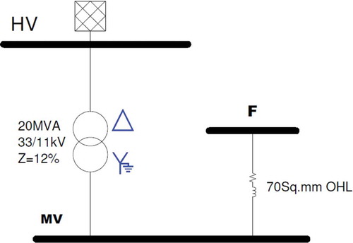
Table 9. Computational results for MV bus voltage

Case	Parameters		Computed MV Bus Voltages
	Zn (Ω)	Zf (Ω)	VA		VB		VC
			kV	Angle	kV	Angle	kV	Angle
a	0.1	35.45	6.32	−30.8	6.31	−150.3	6.40	89.9
b	25.4	35.45	3.74	−29.1	7.88	−167.1	8.07	105.7

Table 10. Computational results for voltages at fault “F”

Case	Parameters		Computed Voltages at Fault “F”
	Zn (Ω)	Zf (Ω)	Va		Vb		Vc
			kV	Angle	kV	Angle	kV	Angle
a	0.1	35.45	6.12	−34.1	6.5	−149.7	6.24	91.1
b	25.4	35.45	3.63	−32.5	7.97	−166.6	8.00	106.4

6. Mathematical modelling and sensitivity calculations

The definition of sensitivity is that when a small change in x produces a large change in the value of a function y = f (x), then the function is relatively sensitive to changes in “x”. The derivative f’ (x) is a measure of this sensitivity (Weir et al.).

The equation $dy=f^{\prime }\left(x\right)dx$ shows how sensitive the output of “f” is to a change in the input “x”.

The sensitivity “S” of “y” to “x” is defined (Hayward & Cruz-Hernandez, 1998; Kuo, 1975) as:

(5) $S_x^y=\frac{\mathrm{\Delta }y/y}{\mathrm{\Delta }x/x}\cong f^{\prime }\left(x\right)\times \frac{x}{y}$(5)

where $f^{\prime }\left(x\right)isexpressedas\underset{h\to 0}{lim}\frac{f\left(x+h\right)-f\left(x\right)}{h}$

The sensitivity “S” is a factor having both magnitude and angle. Regarding the HIF phenomenon in a distribution system, the practical problem is how exactly to detect a HIF; hence, only the magnitude of sensitivity should be considered and analyzed, and the angle is not analyzed in this paper.

6.1. Sensitivity calculation for the fault current I_fa

Differentiating “I_fa” with respect to “Z_f”, Eq. (2)(2) $I_{fa}=3I_{a0}=\frac{V_a}{\left(Z_1+Z_2+Z_0+3Z_n+3Z_f\right)}$(2) becomes

(6) $\frac{\mathrm{\partial }{I}_{fa}}{\mathrm{\partial }{Z}_f}=\frac{-9V_a}{{\left(Z_1+Z_2+Z_0+3Z_n+3Z_f\right)}^2}$(6)

In line with Eq. (5(5) $S_x^y=\frac{\mathrm{\Delta }y/y}{\mathrm{\Delta }x/x}\cong f^{\prime }\left(x\right)\times \frac{x}{y}$(5) ), the sensitivity “S” for fault current “I_fa” with respect to “Z_f” is

(7) $S_{Z_f}^{I_{fa}}=\frac{\mathrm{\partial }{I}_{fa}}{\mathrm{\partial }{Z}_f}\times \frac{Z_f}{I_{fa}}$(7)

(8) $S_{Z_f}^{I_{fa}}=\frac{-3Z_f}{\left(Z_1+Z_2+Z_0+3Z_n+3Z_f\right)}$(8)

A sample calculation of sensitivity S (I_fa) for Z_n = 0.1 ohms and Z_f = 35.45 ohms, the result is

$S\left(I_{fa}\right)=-0.96$.

Figure 17. Sensitivity of fault current S(I_fa) to Z_f = 0.1 to 1000 Ω for different values of “Z_n”. Graph is drawn omitting “θ” (key values are in Table 11).

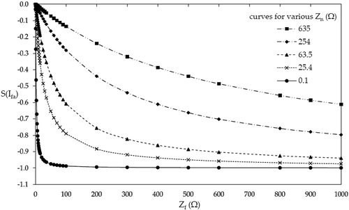
Table 11. Sensitivity of fault current S(I_fa) for different neutral earthing and fault impedances

Zf (Ω)	Zn (Ω)
	0.1	25.4	63.5	254	635
	Sensitivity of fault current S(Ifa)
0.1	−0.03	0.00	0.00	0.00	0.00
10	−0.86	−0.27	−0.13	−0.04	−0.02
35.45	−0.96	−0.57	−0.35	−0.12	−0.05
100	−0.99	−0.79	−0.61	−0.28	−0.14
500	−1.00	−0.95	−0.89	−0.66	−0.44
1000	−1.00	−0.97	−0.94	−0.80	−0.61

The sensitivity of fault current S(I_fa) graph can be analyzed and understood as follows:

• The sensitivity is arrived based on several variables of the real system as in the Eqs. (2)(2) $I_{fa}=3I_{a0}=\frac{V_a}{\left(Z_1+Z_2+Z_0+3Z_n+3Z_f\right)}$(2) , (5(5) $S_x^y=\frac{\mathrm{\Delta }y/y}{\mathrm{\Delta }x/x}\cong f^{\prime }\left(x\right)\times \frac{x}{y}$(5) ) and (8(8) $S_{Z_f}^{I_{fa}}=\frac{-3Z_f}{\left(Z_1+Z_2+Z_0+3Z_n+3Z_f\right)}$(8) ).

• The sensitivity is maximum (that is zero) only when the fault impedance is zero for all ranges of “Z_n”.

• For solid grounded system, the solid line graph with bullets is valid. In this case, the sensitivity is very minimum that is approaching to −1 when “Z_f” increases, for example, S(I_fa) is −0.96.

• The sensitivity value is good when “Z_n” is high, it can be easily seen that the graph for Z_n = 635 ohm is on the top.

6.2. Sensitivity calculation for the line voltage “V_b”

The sensitivity “S” of voltage “V_b” to “Z_f” is calculated using the following derived formula based on Eq. (3)(3) $V_b=\frac{V_a\left(3{\alpha }^2{Z}_f+Z_2\left({\alpha }^2-\alpha \right)+(Z_0+3Z_n)\left({\alpha }^2-1\right)\right)}{\left(Z_1+Z_2+Z_0+3Z_n+3Z_f\right)}$(3) :

(9) $S_{Z_f}^{V_b}=\frac{3Z_f\left(Z_1{\alpha }^2+Z_2\alpha +(Z_0+3Z_n\right)}{D\left(\left(3Z_f{\alpha }^2+Z_2\left({\alpha }^2-\alpha \right)+(Z_0+3Z_n)({\alpha }^2-1\right)\right)}$(9)

Where D = Z₁ + Z₂ + Z₀ + 3Z_n + 3Z_f

The sensitivity of “V_b” to “Z_f” for the real system data given in Section 4 is calculated as

$S_{Z_f}^{V_b}=0.03$ (for Z_n = 0.1 ohm and Z_f = 35.45 ohm)

6.3. Sensitivity calculation for the line voltage “V_c”

The sensitivity “S” of voltage “V_c” to “Z_f” is calculated using the following derived formula based on Eq. (4)(4) $V_c=\frac{V_a\left(3\alpha Z_f+Z_2\left(\alpha -{\alpha }^2\right)+(Z_0+3Z_n)\left(\alpha -1\right)\right)}{\left(Z_1+Z_2+Z_0+3Z_n+3Z_f\right)}$(4) :

(10) $S_{Z_f}^{V_c}=\frac{3Z_f\left(Z_1\alpha +Z_2{\alpha }^2+(Z_0+3Z_n\right)}{D\left(\left(3Z_f\alpha +Z_2\left(\alpha -{\alpha }^2\right)+\left(Z_0+3Z_n\right)(\alpha -1\right)\right)}$(10)

The sensitivity of “V_c” to “Z_f” for the real system data given in Section 4 is calculated as

$S_{Z_f}^{V_C}=0.03$ (for Z_n = 0.1 ohm and Z_f = 35.45 ohm)

From Tables 12 and 13, it can be observed that for high neutral earthing impedance values “Z_n”, the sensitivity of line voltages “V_b” and “V_c” are the same as each other.

Table 12. Sensitivity of line voltage S(V_b) for different neutral earthing and fault impedances

Zf (Ω)	Zn (Ω)
	0.1	25.4	63.5	254	635
	Sensitivity of line voltage S(Vb)
0.1	0.01	0.00	0.00	0.00	0.00
10	0.08	0.13	0.07	0.02	0.01
35.45	0.03	0.19	0.16	0.07	0.03
100	0.01	0.14	0.19	0.14	0.07
500	0.00	0.04	0.09	0.19	0.18
1000	0.00	0.02	0.05	0.14	0.19

Table 13. Sensitivity of line voltage S(V_c) for different neutral earthing and fault impedances

Zf (Ω)	Zn (Ω)
	0.1	25.4	63.5	254	635
	Sensitivity of line voltage S(Vc)
0.1	0.01	0.00	0.00	0.00	0.00
10	0.09	0.13	0.07	0.02	0.01
35.45	0.03	0.19	0.16	0.07	0.03
100	0.01	0.14	0.19	0.13	0.07
500	0.00	0.05	0.09	0.19	0.18
1000	0.00	0.02	0.05	0.14	0.19

The sensitivity results of line voltages S(V_b) and S(V_c), can be analyzed and understood as follows:

• The sensitivity is arrived based on several variables of the real system as in the Eqs. (3)(3) $V_b=\frac{V_a\left(3{\alpha }^2{Z}_f+Z_2\left({\alpha }^2-\alpha \right)+(Z_0+3Z_n)\left({\alpha }^2-1\right)\right)}{\left(Z_1+Z_2+Z_0+3Z_n+3Z_f\right)}$(3) –(5(5) $S_x^y=\frac{\mathrm{\Delta }y/y}{\mathrm{\Delta }x/x}\cong f^{\prime }\left(x\right)\times \frac{x}{y}$(5) ).

• The sensitivity is increasing with increase in fault impedance for higher values of “Z_n”.

• The behavior of sensitivity can be noted from the Tables 12 and 13 that the maximum sensitivity value of 0.19 occurs in each case of “Z_n”.

• For solid grounded system, the sensitivity is close to zero when “Z_f” increases, for example, sensitivity is zero when “Z_f” is 500 ohm or above.

6.4. Sensitivity calculation for neutral voltage “V_n” with respect to neutral earthing impedance

“V_n” is equal to “I_fa” multiplied by “Z_n”;

(11) $V_n=\frac{3V_a}{\left(Z_1+Z_2+Z_0+3Z_n+3Z_f\right)}\times Z_n$(11)

Sensitivity $S_{Z_n}^{V_n}$ is derived based on Eq. (11)(11) $V_n=\frac{3V_a}{\left(Z_1+Z_2+Z_0+3Z_n+3Z_f\right)}\times Z_n$(11) .

$S_{Z_n}^{V_n}=\frac{\mathrm{\partial }{V}_n}{\mathrm{\partial }{Z}_n}\times \left(\frac{Z_n}{V_n}\right)$.

(12) $S_{Z_n}^{V_n}=1-3\frac{Z_n}{\left(Z_1+Z_2+Z_0+3Z_n+3Z_f\right)}$(12)

Similarly, sensitivity of the voltage across the neutral earthing impedance “V_n” with respect to the fault impedance:

$S_{Z_f}^{V_n}=\frac{\mathrm{\partial }{V}_n}{\mathrm{\partial }{Z}_f}\times \left(\frac{Z_f}{V_n}\right)$.

(13) $S_{Z_f}^{I_{fa}}=\frac{-3Z_f}{\left(Z_1+Z_2+Z_0+3Z_n+3Z_f\right)}$(13)

Equations (8)(8) $S_{Z_f}^{I_{fa}}=\frac{-3Z_f}{\left(Z_1+Z_2+Z_0+3Z_n+3Z_f\right)}$(8) and (13(13) $S_{Z_f}^{I_{fa}}=\frac{-3Z_f}{\left(Z_1+Z_2+Z_0+3Z_n+3Z_f\right)}$(13) ) indicate that the sensitivity of the fault current with respect to “Z_f” is the same as the sensitivity of the voltage across neutral earthing impedance values with respect to the fault impedance.

Figure 18. Sensitivity of neutral voltage (V_N) for different values of “Z_n”. Graph is drawn omitting “θ” (key values are in Table 14).

Table 14. Sensitivity of neutral voltage S(V_n) with various neutral earthing impedances

Zf (Ω)	Zn (Ω)
	0.1	25.4	63.5	254	635
	Sensitivity of neutral voltage S(Vn)
0.1	−0.03	0.00	0.00	0.00	0.00
10	−0.86	−0.27	−0.13	−0.04	−0.02
35.45	−0.96	−0.57	−0.35	−0.12	−0.05
100	−0.99	−0.79	−0.61	−0.28	−0.14
500	−1.00	−0.95	−0.89	−0.66	−0.44
1000	−1.00	−0.97	−0.94	−0.80	−0.61

The five sensitivity results for HIFs given in Tables 11–14 and Figures 17, 18 show that the sensitivity of voltage and current are appreciable for high neutral earthing impedance. The implementation of protection relays for faulty circuit isolation can be guided by the variation of sensitivity in the plots of currents and voltages. In the case of a HIF, the voltage across “Z_n” dominates when “Z_n” is high as shown in Figure 18. Over-voltage relays across the neutral and sensitive current relays using a very low CT ratio in a neutral circuit can assist the detection of HIFs in case of a radial line. The application of such protections for multiple lines from a source is not part of this paper. The authors are firm in discriminating faults in multiple lines by applying different design considerations. Such details are not covered in this paper. The emphasis of this paper is on the profiles of the fault system parameters and the sensitivity analysis given. The analysis is not extended beyond 1000 ohms or to multiple fault locations as explained in Section 7. Analysis is also not performed for different power factors of “Z_f” and “Z_n”.

7. Computation of fallen conductor contact resistance and its relation to HIF

To determine the contact resistance (De Sa & Louro, 2010) of a fallen conductor on desert soil, as shown in Figure 19, site-measured desert soil resistivity values using 4-point Wenner method as in Table 15 were used in a CymGRD software simulation. The simulation results are given in Table 16. The computed results support the high-fault impedance values chosen in the analysis.

Figure 19. Representation of a fallen conductor in high-resistivity desert soil.

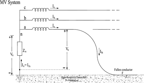
Table 15. Site-measured desert soil resistivity

SI. No	Probe Distance (m)	Resistance (Ohms)	Resistivity (Ohm-m)
1	1	637	4002
2	2	280	3521
3	3	147	2771
4	5	44	1397
5	7	14	631
6	9	5	289
7	10	3	203
8	12	2	115
9	15	1	72
10	20	0.5	59

Table 16. Computed contact resistance of a fallen conductor

Input Parameters for simulation
Conductor size	: 70 Sq.mm (Al)
Conductor Length	: 10 m
Upper Layer Thickness	: 0
Upper Layer Resistivity	: 4002 ohm-m
Lower Layer Resistivity	: 4002 ohm-m
Output Result from the software simulation
Calculated Ground Resistance	: 885.955 ohm

The top desert soil has a resistivity (Velmurugan, 2012) value of 4002 ohm-m, and the computed contact resistance of a 10-m, 70-mm² Al conductor is approximately 886 ohms, as shown in Table 16. Hence, sensitivity analysis is carried out for various fault impedances (0.1–1000 ohms). The soil the nature of fault impedance is resistive, as per the CymGRD software results. On-site measured live line-to-ground-fault current is very minimal in either amperes or fractions of amperes. In some cases of field measurements conducted in desert region (Velmurugan, 2012), fault currents in some locations could not be measured even with very sensitive instruments, which means that the contact resistance of the fallen conductor is several thousand ohms.

8. Conclusions

The analysis in this paper has been conducted based on the theory of symmetrical components, which is founded on the time sequence of signals. However, after manipulating the equations, the obtained results largely indicate the contribution of space to the fault current and healthy phase voltages. The deeper meaning of space is the behavior of soil in permitting low-fault current to pass through it. As the fault current “I_fa” is not influential in high-impedance cases, faulty circuit isolation cannot be entirely ensured by a relay circuit in a neutral system. Such critical phenomena can be monitored by using background knowledge involving the variation of the sensitivity of fault currents and healthy phase voltages with respect to fault impedance.

• From the mathematical analysis, it is clearly observed that under the influence of HIFs, the voltage across the neutral impedance becomes high when “Z_n” is increased.

• Over-voltage relays at the source end, in conjunction with a low-CT circuit for sensing zero-sequence current, can guide the detection of HIFs.

• The application of a low CT ratio requires a high resistance earthed neutral system. Thus, the results of the sensitivity analysis lead us to focus on the neutral zone and bus voltages of the source instead of unnecessary searches for wider areas.

• In this research paper, limited live line test results are presented. However, as far as the validity of the analytical results using symmetrical components theory is concerned, they closely match the live line test results. Even though the foundation of the current work is based on a field problem, only relevant information has been referred to. The sensitivity of HIF can be expressed, in real situations, as a more important fact by moderating the neutral earthing impedance.

• This research paper concludes that the distribution system applying neutral earthing impedance will certainly aid in detection of high impedance faults in desert regions.

• The sensitivity analysis can be extended to isolated power systems using dedicated generators (application of such generators by itself can be a future study) to feed to desert regions, and in this case the sensitivity analysis could point to tuning more parameters such as reactances of generator in addition to tuning neutral earthing impedance.

• In cases where the fallen conductor does not exceed the minimum required zero-sequence current, the fault is an open-circuit fault (although it can be classified as a single-phase-to-ground fault); then, the monitoring of the line from the far end should be considered.

  Nomenclature

  A	Ampere
  kA	Kilo-amp
  Al	Aluminium
  VA, VB, VC	Bus voltages
  IA, IB, IC	Phase currents
  Z	Circuit impedance
  Zf	Fault impedance
  θ	angle (in degrees)
  Va, Vb, Vc	Line voltages at fault “F”
  Zn	Neutral earthing impedance
  Ω	Ohm
  Va	Phase-to-ground voltage
  Z1, Z2, Z0	Positive-, negative-, zero-sequence impedance
  Ifa	Single-phase-to-ground fault current
  S	Sensitivity
  Zs	Source impedance
  Zt	Transformer impedance
  V	Volts
  kV	Kilovolt
  Abbreviation
  G	Generation
  HV	High Voltage (33 kV)
  ST	Station Transformer
  CT	Current Transformer
  D	Detection Device
  MV	Medium Voltage (11 kV)
  VT	Voltage Transformer
  L	LV Load via step down transformer
  DT	Distribution Transformer
  LV	Low Voltage
  F	Fault
  NOP	Normally Open-Point
  HIF	High Impedance Fault
  OHL	Overhead line
  DWT	Discrete wavelet transform
  ANFIS	Adaptive neuro-fuzzy inference system
  EMTP	Electromagnetic transient program
  ETAP	Electrical transient and analysis program
  PSCAD	Power system computer-aided design
  MATLAB	Matrix laboratory

Additional information

Funding

The authors received no direct funding for this research.

Notes on contributors

Perumal Velmurugan

Mr. Perumal Velmurugan born in Tamil Nadu State, India in 1962. He received BE degree in Electrical and Electronics Engineering from College of Engineering, Guindy in 1984 and ME degree in Power System Studies from Annamalai University, Tamil Nadu in 1990. He is currently a Research Scholar in BITS-Pilani, Dubai Campus in the area of Detection of High Impedance Fault (DoHIF). Author possesses an extensive experience of over 33 years in Power Generation, Transmission and distribution including Power System Analysis using various softwares. He worked as Lead Protection Engineer in a rare kind of project in UAE: Live line to ground fault short circuit tests on 11kV OHL and Experimental Earthing System in desert areas. He represented as a Chairman at technical workshops. He is a member of IEEE, Society of Engineers UAE. He is current working as Engineering Manager in TWINVEY Electric Consultancy, Dubai.

References

- ABS Mohamed Rayees, Velmurugan Mariappan, & Maha AlDahmi (2014). Earthing System Analysis to Improve Protection System Performance in Distribution Networks. 12th IET International Conference on Developments in Power System Protection (DPSP 2014). https://doi.org/10.1049/cp.2014.0092
- Apostolov, A. P., Bronfeld, J., Saylor, C. H. M., & Snow, P. B. (1993). An artificial neural network approach to the detection of high impedance faults. International conference on expert system applications for the electrical power industry proceedings.
- Balser, S. J., Clements, K. A., & Kallaur, E. (1982). Detection of high impedance faults (EPRI Final Report, EPRI EL-2413).
- Balser, S. J., Clements, K. A., & Lawrence, D. J. (1986). A microprocessor-based technique for detection of high impedance faults. IEEE Transactions on Power Delivery, PER-6(7), 59–23. https://doi.org/10.1109/MPER.1986.5527876
- Boudjit, K., Korzet, W., Nacer, A., Moulai, H., & Larbes, C. (2012). DSP use in distribution power grids - a new approach for high impedance Arc faults detection. IEEE in electrical systems for aircraft, railway and ship propulsion. https://doi.org/10.1109/ESARS.2012.6387477
- Carr, J., & Hood, G. L. (1979). High impedance fault detection on primary distribution systems (CEA Final Report, Project No. 78–75).
- Chakraborty, S., & Das, S. (2018). Application of smart meters in high impedance fault detection on distribution systems. IEEE Transactions on Smart Grid, 10(3), 3465–3473. https://doi.org/10.1109/TSG.2018.2828414
- Costa, F. B., Souza, B. A., Brito, N. S. D., & Silva, J. A. C. B. (2015). Real-time detection of transients induced by high impedance faults based on the boundary wavelet transform. IEEE Transactions on Industry Applications, 51(6), 5312–5323. https://doi.org/10.1109/TIA.2015.2434993
- Cui, Q., El-Arroudi, K., & Weng, Y. (2019). A feature selection method for high impedance fault detection. IEEE Transactions on Power Delivery, 34(3), 1203–1215. https://doi.org/10.1109/TPWRD.2019.2901634
- Das, R., & Bayoumi, D. (2007). System for detection of high impedance fault. 19th international conference on electricity distribution.
- De Sa, J. L. P., & Louro, M. (2010). On human life risk-assessment and sensitive ground fault protection in MV distribution networks. IEEE Transactions on Power Delivery, 25(4), 2319–2327. https://doi.org/10.1109/TPWRD.2010.2053564
- Ebron, S., Lubkeman, D. L., & White, M. (1990). A neural network approach to the detection of incipient faults on power distribution feeders. IEEE Transactions on Power Delivery, 5(2), 905–914. https://doi.org/10.1109/61.53101
- Ghaderi, A., & Mohammadpour, H. A. (2017). High impedance fault detection: A review. Electric Power Systems Research, 143, 376–388. https://doi.org/10.1016/j.epsr.2016.10.021
- Gomes, D. P. S., Ozansoy, C., & Ulhaq, A. (2018). High-sensitivity vegetation high impedance fault detection based on signal’s high-frequency contents. IEEE Transactions on Power Delivery, 33(3), 1398–1407. https://doi.org/10.1109/TPWRD.2018.2791986
- Grainger, J. J., & Stevenson, W. D. (1994). Power system analysis. Jr. McGraw-Hill Series in Electrical and Computer Engineering, International Edition.
- Hayward, V., & Cruz-Hernandez, J. M. (1998). Parameter sensitivity analysis for design and control of force transmission systems. ASME Journal of Dynamic Systems, Measurement, and Control, 120(2), 241–248. https://doi.org/10.1115/1.2802415
- IEEE Power Engineering Society, Downed Power Lines. (1989). Why they can’t always be detected. IEEE.
- Jeerings, D. I., & Linders, J. R. (1991). A practical protective relay for down-Conductor faults. IEEE Transactions on Power Delivery, 6(2), 565–574. https://doi.org/10.1109/61.131113
- Jota, F. G., & Jota, P. R. S. (1998). High-Impedance fault identification using a fuzzy reasoning system. IEE Proceedings – Generation, Transmission and Distribution, 145(6), 656–661. https://doi.org/10.1049/ip-gtd:19982358
- Kim, C. J., & Russell, B. D. (1989). Classification of faults and switching events by inductive reasoning and expert system methodology. IEEE Transactions on Power Delivery, 4(3), 1631–1637. https://doi.org/10.1109/61.32653
- Kothari, D. P., & Nagrath, I. J. (2007). Power system engineering (Second ed.). Tata McGraw-Hill Publications.
- Kuo, B. C. (1975). Automatic control systems (Third ed.). Prentice-Hall Inc.
- Lai, T. M., Snider, L. A., & Lo, E. (2006). Wavelet transformation based algorithm for the detection of stochastic high impedance faults. Proceedings of the Electric Power Systems Research, 76(8), 626–633. https://doi.org/10.1016/j.epsr.2005.12.021
- Lee, I. (1982). High impedance fault detection using third harmonic current (EPRI Final Report, EPRI EL-2430). Palo Alto, Calif. : The Institute, ©1982.
- Louro, M., & De Sa, J. P. (2007). Evaluation of protection approaches to detect Broken conductors in distribution networks. 19th international conference on electricity distribution.
- Masa, A. V., Maun, J.-C., & Werben, S. (2011). Characterization of high impedance faults in solidly grounded distribution networks. 17th power systems computation conference-Stockholm Sweden (pp. 22–26). https://api.semanticscholar.org/CorpusID:18310281
- Papathanassiou, S., Tsili, M., Georgantzis, G., & Antonopoulos, G. (2007). Enhanced earth fault detection on MV feeders using current unbalance protection. 19th international conference on electricity distribution.
- Russell, B. D., Aucoin, B. M., & Talley, T. J. (1982). Detection of arcing faults, on distribution feeders (EPRI Final Report, EPRI EL-2757).
- Sheng, Y., & Rovnyak, S. M. (2004). Decision tree-based methodology for high impedance fault detection. IEEE Transactions on Power Delivery, 19(2), 533–536. https://doi.org/10.1109/TPWRD.2003.820418
- Song, X., Gao, F., Chen, Z., & Liu, W. (2019). A negative selection algorithm-based identification framework for distribution network faults with high resistance. IEEE Access, 7, 109363–109374. https://doi.org/10.1109/ACCESS.2019.2933566
- Tengdin, J., Westfall, R., & Stephan, K. (1996). High impedance fault detection technology. IEEE power system relaying committee working group D15 report.
- Velmurugan, P. (2012). Test Reports on Trial Earthing in AADC Network. TWINVEY Electric Consultancy.
- Weir, M. D., Hass, J., & Giordano, F. R. Thomas’ Calculus (Eleventh ed.). Pearson Education.
- Yang, M.-T., Gu, J.-C., Hsu, W.-S., Chang, Y.-C., & Cheng, C. (2004). A novel intelligent protection scheme for high impedance fault detection in distribution feeder. IEEE region 10 conference TENCON 2004. https://doi.org/10.1109/TENCON.2004.1414792
- Zamanan, N. (2007). Arcing high impedance fault detection using real coded genetic algorithm. Proceedings for third IASTED Asian conference power and energy systems. https://api.semanticscholar.org/CorpusID:55490786
- Zamora, I., Mazo´n, A. J., Aginako, Z., & Buigues, G. (2012). Low-current fault detection in high grounded distribution networks, using residual variations of asymmetries. IET Generation, Transmission & Distribution, 6(12), 1252–1261. https://doi.org/10.1049/iet-gtd.2012.0195
- Zamora, I., Mazo´n, A. J., Sagastabeitia, K. J., Pico´, O., & Saenz, J. R. (2002). Verifying resonant grounding in distribution systems. IEEE Computer Applications in Power, 15(4), 45–50. https://doi.org/http://dx.doi.10.1109/MCAP.2002.1046111