Freight route planning in intermodal transportation network to deal with combinational disruptions

Abstract

In this study, we developed an intermodal transportation model that extends the VRP model and its recovery model. This study emphasizes re-identifying the best route, departure time, and the selection of the best ship with the right type of capacity booking that produces the lowest total cost after dealing with disruption. The re-routing process is shifted by transforming the disruption to a virtual node in order to define the added time and cost after a disruption occurred. The disruption types include link and customer disruptions. The numerical experiment uses the metaheuristics, namely, Genetic Algorithm and Simulated Annealing, because it is an np-hard problem. The results of the optimization process yielded the total cost increased when the average vehicle speed was enhanced. The starting service time provides cost savings through a reduction of penalties because the arrival is not within the time window that had been agreed upon. Besides, the type of capacity order, more specifically the type of direct purchase (on the spot), provides better costs when the level of disruption is heavy. In contrast, a lighter level of disruption can cause a minimal total cost for purchasing the up-front type of fee. However, the scenario of capacity cost shows that lower prices can make the direct purchasing type more profitable. On the other hand, increasing the price of renting a ship’s capacity makes the up-front type of fees more profitable.

Keywords:

• customer disruptions
• link disruptions
• intermodal
• freight routing planning
• capacity booked
• time appointment
• genetic algorithm
• simulated annealing

PUBLIC INTEREST STATEMENT

There are various optimization procedures investigated to handle and control disruptions in the process of shipping goods in intermodal transportation. It still needs an in-depth investigation because the disruptions type and effect are uncertain and tend to cost a lot. This paper proposes the intermodal freight routing planning problem with considering combinational disruptions. Beside propose the metaheuristic optimization technique to solve this np-harp problem, we also propose the combinational disruptions transformation procedure. Besides, this paper points out that the contract strategy, the starting service time strategy, and the vehicle scheduling strategy are the key point to arrange the best route and minimization of the total cost deviation from disruptions impact in this area problem. Then from the optimization view, our numerical experiment shows that SA methods give better results than GA.

1. Introduction

There are various vehicle route planning problems, and they can be more complex when the objective functions and constraints are increased. Then, optimal solutions should be developed to solve the routing problems. The routing problem model underwent various developments in more complex objective functions and constraints. Initialized by a single objective until multi-objective or starting from the original vehicle routing problem (VRP) to a VRP considering capacity, time windows, hard time windows, backhaul, and several other restrictions can be more complex and need to be solved. On the other hand, the optimization of routing in intermodal transport networks has emerged in recent years. The development of a route model is based on the type of mode, the type of uses for the modes, namely transport of goods or passengers, and intermodal synchronization. In addition, system constraints studied are extended TSP or VRP, door to door delivery, door to port delivery, port to door delivery, etc. Also, based on system conditions, the development of research on route problems in intermodal transportation networks has evolved from deterministic route problems to route problems that consider uncertain or dynamic systems.

Some paper investigated an incident that makes the system became uncertain and mentioned this event as disruptions. A Disruption is an event that can significantly affect system performance. In this study, the disruptions are investigated based on the source of the activity interruption. Posit the provenance of the disruptions in supply chains; it divided into vehicle breakdowns, link disruptions, supply disruptions, and customer disruptions (Eglese & Zambirinis, 2018; Li & Li, 2020; Wang et al., 2012). In this study, the researchers focus on two sources of disruptions: link disruptions and customer disruptions.

A Link disruption is a type of disruption where the impact is a disruption in a link of the network. The impact scope of this type of disruption is a disruption that disrupts the link itself until some links that connect with a link are disrupted (Kim et al., 2015). The link disruption can be due to accidents, breakdown or failure of vehicles, natural disasters, extreme weather, terrorists, and road facilities improvements. These disruptions are very common and affect not only the distribution system but also the production system (Li & Li, 2020). The effects of these disruptions vary. For example, extreme weather can cause flooding; natural disasters may damage a road, and there are disruptions from accidents, vehicle breakdowns or terrorists. Those incidents often stimulate congestion. Managing the impact of these disruptions is very important especially when facing the damage impact of disruptions.

Customer disruptions are the disruptions caused by the customer that include changes in demand in terms of the quantity or type of product, changes in customer locations, and changes in a customer’s time window (Wang et al., 2012). The main factor of customer disruptions is the demand change. The fluctuation of demand change gives the risk in the system (Zhao et al., 2020). The demand change from customers will affect the shipping plan that has been made, so it needs to be revised. Both the number and type of goods significantly affect the repeat decision for shipping in order to anticipate the volatile demand. When increasing the amount ordered or the addition of new types of goods occur, then re-planning done by a modification of the last route plan and adding a new container assignment. This can increase the total cost. On the other hand, reducing demand can decrease profits. Besides, re-planning a change in the delivery time window or a change in the destination (delivery address) changes the composition of the delivery assignment if the goods are similar and the capacity can fulfil the demand.

There are two approaches to study disruptions. First, flow-based importance is based on the size of the link centrality (between centrality) that analyzes the level of use of the link in the traffic flow (Jenelius, 2010). Secondly, there is impact-based importance. This is based on the impact of the disruption. Some researchers have studied how the impact originated. Namely, they analyzed network resilience through the link’s average use, a size indicator to count the increasing travel costs (Ishfaq, 2012) and traffic/commodity flow (Jenelius, 2010; Leal et al., 2014; Starita et al., 2016). Besides, Rosyida et al. (2019) analyzed the impact of this type of disruption in the analysis of vehicle routes through scenarios of changes in vehicle speed levels.

Many studies have investigated the strategy to deal with a disruption without considering the logistical factors, namely customers, drivers, and logistics providers. A limited number of previous studies have considered these factors even though in reality they are influential. Eglese and Zambirinis (2018) stated that good communication between the logistical operators is important especially when facing disruptions. This will bring good recovery plans, such as real-time recovery plans. This problem still needs investigation in order to find the best method of communication management and develop an optimization method. Furthermore, a powerful computer is needed to support real-time purpose.

In an intermodal transportation network, a discussion about this disruption began to attract many researchers related to the uncertainty. Rosyida et al. (2018) classified many previous studies based on the graph theory, the way of disruption conversion, methods (such as metaheuristic, optimization or simulation), and strategies to solve the disruptions. According to Rosyida et al. (2018), there is still a need for investigation to know the strategies to anticipate the disruption. The strategies include routing strategies, mode selection, contract selection for book capacity on ships, and other shipping strategies. Determination of strategy selection can significantly affect the optimization of the total costs required. Besides, many previous papers discussed the transportation of goods on an intermodal transportation network. Both mathematical models and simulations in the logistics/shipping processes are included in order to model the intermodal transportation systems.

Those papers investigated the transfer process between mode, route selection, etc. Behdani et al. (2016), Agbo et al. (2017), and Agbo and Zhang (2017) studied the transfer process between mode and intermodal synchronization schemes. While Sitek et al. (2020), Shao and Dessouky (2020), Zeng et al. (2020), and Gohari et al. (2018) investigated routing selection. Sun et al. (2015) discussed optimization models for freight routing planning problems (FRPP) on multimodal transport networks and present algorithms to complete the development of the FRPP model. Sun et al. (2015) examined each mathematical formulation in the FRPP model starting from the object for optimization (single or multi-commodity), commodity type (splittable or unsplittable), network resource type (capacitated or uncapacitated), transportation pattern type (single or multi), the optimization criteria (single or multi) and the type of case being analyzed (deterministic or stochastic). According to Sun et al. (2015), the mathematical model of FRPP for the case of uncertainty and multiple services still needs to be investigated. Also, there is a research agenda to further investigate the delivery time related to inventory or the capacity usage.

In an intermodal transportation network, logistics players include terminal operators, freight forwarders, carriers and customers. Each of these actors aims to make sure that their system has optimal performance. Terminal operators always want to improve the performance of their operating systems. One of the strategies is to use a truck appointment system management to anticipate excessive queues at the terminal process. The truck appointment system aims to minimize the truck waiting time at the terminal by setting a time window for each truck to enter the terminal. This time window is needed to reduce the number of trucks entering at the peak time so that the waiting time can decrease (Phan & Kim, 2015; Shiri & Huynh, 2016; Torkjazi et al., 2018; Zhang et al., 2019). On the other hand, freight forwarders try to get the least possible shipping costs by planning the right route or delivery schedule. Meanwhile, the carrier optimize the customers of the vessel with the capacity offered. Offering payment ordering scheme strategies to customers is used to make all capacities sold (Widjanarka et al., 2018). Finally, on the customers’ side, they need flexibility in ordering and requesting changes to an order. The flexibility includes changes in the number requested, delivery locations, delivery times, or other changes (Pi et al., 2019; Wang et al., 2012; Zhao et al., 2020). The variety of intermodal logistical player purposes gives the challenge to choose the best strategy when facing disruptions. Some papers discussed coordination and collaboration strategy to solve this problem.

In this study, an extension of the VRP model is developed. The model identified the optimal conditions in terms of the freight forwarder by considering the optimal criteria of other actors when disruptions occur. This study analyzes strategic decisions in order to adapt to disruptions that can influence a transportation network. Therefore, this alternative strategy can solve the disruption problem and can find the optimal solution. However, it is also necessary to do analysis when choosing a new strategy. This is a study of the decision-making process for selecting the best alternative when facing a disruption.

Based on the above background, we investigated the optimization of an intermodal freight routing planning problem (IFRPP) model that considers combinational disruptions. The novelty of this research is in three areas. 1) The IFRPP model is an extension of the VRP model that considers two modes for combinational disruption cases. In this model, we consider the time window constraints on the customer node and the time window limits at the port. There are two types of time window limits at ports; one time window refers to truck appointments to limit the time of trucks entering the terminal and the second time window relates to the process of loading containers. Besides, there are two types of ship capacity booking costs, including an upfront fee and on the spot fee. On the disruptions side, the disruption type considered is a combination of customer disruptions and link disruptions. Customer disruptions include changes in demand and changes in the location of the delivery destination and the customer time window. Link disruptions cause link performance to decrease and the average speed of the vehicle also decreases. This decline in performance comes from an extreme weather event in the form of heavy rain that causes puddles that affect road performance. 2) We extend the IFRPP model to the recovery of IFRPP model. 3) We consider the step of combinational disruptions transformation procedure that can be used to analyze the disruptions’ impact.

The rest of this paper organized as follows. In section two, we discuss the problem statement. In section three, we present a model formulation. In this section, we explain the mathematical model and the model assumptions. In section four we explain the methodology. The next section, section five, we provide the numerical experiments. Results and the discussion are presented in section six. In the last section, we discuss the conclusions and further research for this study.

2. Statement of problem

2.1. Problem definition

The intermodal transportation network consists of several nodes (n) and an edge (e). The connection between a node and edge is illustrated in Figure 1. In Figure 1, the node describes the location of the supply/depot (origin node), port, and customer (destination node). On the other side, the edge illustrates the means of transportation that consists of a roadway and a sea way. In Figure 1, the origin node is a shipper that sends its goods to several customers with several containers. The provider/freight forwarder is a transportation service that sends goods from the location of the shipper to the location of the destination or customer (consignee). The terminal is a node used for the transfer from a land mode to a sea mode, or otherwise.

Figure 1. Intermodal supply network.

In this study, the delivery process considers a disruption that significantly affects system performance. The types of disruptions are customer disruptions and link disruptions. Customer disruptions include customer demand changes, customer time window changes, and customer location changes. On the other hand, a link disruption is a disruption caused by an incident that affects highway performance. When the highway performance decreases, the average vehicle speed has the same condition. In this case, heavy rain that produces a pool of water on a highway causes highway performance to decrease. The value of this disruption is converted to the depth of the pool of water due to heavy rain. Based on that depth of water, the vehicle speed level on the highway can be counted. (Pregnolato et al., 2017). In the optimization model, the disruption transformation is used to define the impact of disruptions in the system. Adding a new node as a virtual customer or virtual transit node is a way of disruption transformation. For customer disruptions, a virtual customer is created to accommodate changes in customer demand data (Wang et al., 2012).

In contrast, the two virtual nodes are used to accommodate the link disruption. First, a virtual disruption node is used to accommodate the location of the disruption. The second node, the virtual transit node, is used to accommodate the in-transit vehicle location. This node is the spot when the trucks from the depot face congestion that comes from the disruption node. The distance between both nodes, the disruption node and in-transit vehicle node, can be calculated with the Euclidean distance equation. Besides, the sum of travel time is counted by using the average speed as a scenario. In addition, in the case of combinational disruptions, the transformation processes involve three types of nodes. The first node is to accommodate the disruption spots, the second node is to accommodate the in-transit vehicle location, and the last node is to accommodate the in-transit of a new vehicle when it faces the disruptions.

Because the disruption event is an uncertain condition, a strategy is needed to keep the system stable. The chosen strategy is a flexible shipment strategy. This flexibility strategy creates additional costs and time in the shipment process. Additional costs incurred include transportation costs, transfer fees, and waiting costs that are charged in the shipment process because the shipment arrives before or after the set time window. In contrast, the additional time that arises includes transportation time, transfer time, and waiting time due to arriving too early or arriving late for a predetermined schedule.

The flexible strategy must balance with an efficient strategy to obtain equilibrium in the decision-making process. The efficiency of arrival time at the terminal is in the form of a strategy for determining the optimal departure time from the shipper location. This strategy ensures the arrival of each truck at the terminal will be according to the appointment time agreed upon between the service provider and the terminal operator. The ranges of time appointments are taken from journals that discuss time appointment optimization at the port. Penalties are imposed when the truck does not meet the appointment time. The amount of the penalty fee is per unit of the time window.

Besides, this model also analyzes the ordering capacity strategy in the seaway when faced with disruptions. There are two types of capacity orders, namely booking capacity first and purchases directly at the terminal. The type of purchase affects the capacity price per twenty-foot equivalent unit (TEU). According to Widjanarka et al. (2018), booking capacity ensures the availability and gives a cheaper cost, but the shipper must pay the booking fee in advance, 30% of the capacity cost per TEU, and these costs will be lost if there is a cancellation of capacity usage. The other type of capacity order gives a different cost or random cost.

2.2. Notation and assumptions

The explanation of the mathematical model consists of an explanation of assumptions, notations, and variable descriptions. Assumptions used in this model include the following:

1. This model considers one origin and multiple destinations.

2. This system consists of one node as a depot, two nodes as terminals, and several nodes as delivery locations. The depot is the origin node that connects directly to the terminal node. A customer node is connected to the terminal destination.

3. The modes of transportation considered are trucks and ships.

4. Intermodal synchronization considered is the timeliness of trucks at the terminal based on the agreed time window (according to the contract).

5. The ship arrival time is not considered and the ship is assumed to be ready to depart according to the scheduled time.

6. The disruptions are considered as a customer disruption and a link disruption. The link disruption occurs in the roadway, which caused the average speed of each truck to decrease. Decreased levels from these averages are based on data reported by Pregnolato et al. (2017). In this paper, the location of the link disruption is determined, and the process of determining the coordinates of the link disruption location is not considered.

7. This model does not consider the calculation of the conversion of the disruption to the average level of vehicle speed. The model analyzes the possible impact of this reduced rate on the total system cost.

8. A combination of disruptions occurs at the same time.

The notation of the mathematical model consists of indexes, sets, parameters, decision variables, and derived variables. The notations are explained below:

Index:
$n_1$	=	Terminal Index
$n_2$	=	Customer Index
$n_o$	=	Depot, terminal, and customer index
K	=	Container index
M	=	Mode index

Sets:
$N_1$	=	Set of terminal node, $N_1$= {1, 2, … …,a}
$N_2$	=	Set of customer node, $N_2$ = {1 +a, 2 +a, … … b +a}
$N_o$	=	Set of all node (depot, terminal, customer), $N_0=\left\{0\right\}{\cup }^{N_1}{\cup }^{N_2}$
K	=	Set of container, K ={1,2, … .,k}
M	=	Set of mode, M ={1,2}, 1 =truck; 2 =ship
T	=	Set of ship departure in terminal, T = {1, 2, … …, t}.

Parameter:
$c_{ijkm}$	=	Transportation cost from node I to j with container k and mode m, $i,j\in N_0$
${\theta }_{jkm}$	=	Container loading cost in terminal for container k in node j and mode m.
${\beta }_2^{\hspace{0.17em}}$	=	Penalty cost for early arrival per unit time window.
${\beta }_1^{\hspace{0.17em}}$	=	Penalty cost for lateness arrival per unit time window.
$q_k$	=	Maximum capacity of container k.
$d_i$	=	Customer demand, $d_0;d_1;d_2=0$
$T{o}_{mt}^j$,$T{c}_{mt}^j$	=	Time Window in node j
$Tcma{x}_{mt}^j$	=	Closing time for stacking period t
$T_{ijkm}$	=	Transportation time of a shipment in a link (i,j) using container k and mode m., $i,j\in N_0$
$se{r}_{ikm}$	=	Service time for loading/unloading of container k and mode m in node i.
M	=	Big Number
$\xi$	=	Range of time window per-period.
£	=	Terminal operational time per-day
Τ	=	Container delay tolerance to entrance terminal
$TDpla{n}_{ikm}$	=	Time departure of container k with mode m in terminal j
$Tre{q}_{jkm}$	=	Maximum time arrival requirement of container k with mode min node j

Decision Variable:
$x_{ijkm}$	=	Binary variable. $x_{ijkm}=$ 1, if container k shipment in link (i,j) use mode m, otherwise $x_{ijkm}$=0
$lw{d}_{jkm}^1$	=	Binary variable. $lw{d}_{jkm}^1=$ 1, if arrival time of container k that shipment in link (i,j) with mode m exceed from time window 1, otherwise $lw{d}_{jkm}^1=$=0
$lw{d}_{jkm}^2$	=	Binary variable. $lw{d}_{jkm}^2=$ 1, if arrival time of container k that shipment in link (i,j) with mode m exceed from time window 2,, otherwise $lw{d}_{jkm}^2$=0
${\delta }_{jkm}$	=	Binary variable. ${\delta }_{jkm}=$ 1, if shipment of container k changes transportation mode at node j, otherwise ${\delta }_{jkm}=$ 0
$U_{ikm}$	=	Binary variable. $U_{ikm}=$ 1, if shipment of container k with mode m visit node i, otherwise $U_{ikm}$=0

Derived Variables:
$T{A}_{jkm}$	=	The arrival time of container k use mode m in node j
$T{D}_{ikm}$	=	The departure time mode m in node i that used container k.
$e{w}_{jkm}^{\hspace{0.17em}}$	=	The waiting time caused by the earliness of container k use mode m that arrives at terminal j before$T{o}_{mt}^j$
$l{w}_{jkm}^{\hspace{0.17em}}$	=	The waiting time caused by the lateness of container k use mode m that arrives at terminal j after $T{c}_{mt}^j$

3. Model formulation

The mathematical model consists of two models, namely the original model and the recovery model. The model is intended to find the optimal cost of the shipping process from the depot to the customer by using two modes of transportation, namely trucks and ships. In the transfer process at the terminal, two conditions are considered, namely the time appointment of the terminal system and the capacity contract rule of the carrier. As explained in section 2, concerning the two conditions are considered, the optimal cost and its sensitivity value that is sought when a disruption occurs and affects the system. The disruptions are in the form of link disruption and customer disruption. The time of the disruption in this research is when the shipping process has run from the depot to the terminal. The disruptions convert to time trough the disruption transformation process, as described in section 2.

3.1. Original model

The mathematical model for the freight routing planning problem of an intermodal transportation network is described as (1)—(22).

3.1.1. Objective function

The objective of this model is to minimize shipping costs incurred by freight forwarders, which include transportation costs for each vehicle on a highway, capacity fees for ship modes, transfer fees at the terminal, and penalty fees at the terminal for breaking the time window.

(1) $\begin{array}{rl}& minZ={\sum }_{\left(i,j\right)\in N_o,k\in K,m\in M}{c}_{ijkm}{X}_{ijkm}+{\sum }_{\left(i,j\right)\in N_o,k\in K,m\in M}\left(0,3c_{ijkm}{X}_{ijkm}\right)+\\ & \left(0,7c_{ijkm}{X}_{ijkm}\right)(1-lw{d}_{jkm})+\left(c_{ijkm}{X}_{ijkm}+c_{ijkm}{X}_{ijkm}\right)lw{d}_{jkm}+{\sum }_{j\in N,k\in K}{\delta }_{jk}{\theta }_{jk}+\\ & {\sum }_{j\in N,k\in K,m\in M}{\beta }_{1}e{w}_{jkm}+{\beta }_{2}l{w}_{jkm}\end{array}$(1)

The objective function includes the total transportation costs used by the truck transportation mode to deliver containers from the depot to the terminal and from the terminal to several customers. The second cost element is the capacity cost that consists of 30% paid when ordering the vessel capacity and the remainder paid after using the ship’s services. If the capacity is cancelled, the 30% of the booking fees paid are lost. The third element of the model’s objective is the transfer fee at the terminal, which is the cost used for the loading/unloading process of two modes, the truck and ship. The fourth cost element is the penalty fee that must be paid by the trucking company to enter the terminal if it violates the agreed time window appointment with the terminal. The penalty fee will be charged to a truck when it arrives earlier than the agreed time of entry or if it arrives after the agreed maximum entry time. The unit time for a truck waiting in the terminal determines the value of the delay based on the calculation of the total time of the delay or early arrival divided by the total unit time window.

3.1.2. Flow constraint

(2) ${\sum }_{k\in K,m\in M}{U}_{ikm}=1fori\in N_2$(2)

(3) ${\sum }_{k\in K,m\in M}{U}_{ikm}\le Kfori=\left\{0,1,2\right\}$(3)

Constraint (2) shows the flow constraint of the container in the customer node that will only be passed once by container k using mode m. The above constraints only apply to customer nodes. $U_{ikm}$ is a binary variable that will be 1 if node i is visited by containers k and mode m and is 0 if the condition is the opposite. Constraint (3) shows the flow constraint for the depot node and terminal nodes. Included within this constraint is that all those nodes are passed fewer than k containers, and the total number of containers is less than the total containers in the depot.

(4) ${\sum }_{l-0,l\ne i}^N{X}_{likm}={\sum }_{j-0,j\ne i}^N{X}_{ijkm}=U_{ikm}forN=N_0,k\in K,m\in M$(4)

(5) ${\sum }_{j=3}^N{\sum }_{k=1}^K{\sum }_{m=1}^M{X}_{2jkm}={\sum }_{i=3}^N{\sum }_{k=1}^K{\sum }_{m=1}^M{X}_{i2\text{primekm}}\le K$(5)

Constraint (4) is a constraint stating that the number of containers entering the depot, terminal, and customer nodes is the same as the number of containers coming out of these nodes. Constraint (5) is a constraint stating that the numbers of containers leaving terminal 2 are confirmed to return to terminal 2, and the amount is less than the total containers owned by the depot.

(6) ${\delta }_{jkm}\ge {\sum }_{i\in N_1{\cup }^{N_2}}{X}_{ijkm}-{\sum }_{i\in N_1\cup N_2}{X}_{jikm}fork\in K,j\in N_1\cup N_2,m\in M$(6)

Constraint (6) is a statement about the transfer process when the mode change occurs. The value ${\delta }_{jkm}$ is 1 if a mode change occurs, and it has a value of 0 if no mode change occurs.

3.1.3. Capacity constraint

The capacity constraint is intended to limit the capacity use of the mode. This study only discusses container capacity, whereas the capacity of the ship is not considered.

(7) ${\sum }_{i=1}^{N_2}{d}_i\times U_{ikm}\le q_{k}fork\in K,m=\left\{1\right\}$(7)

Constraint (7) states that the number of customer requests served by container k must be less than the capacity of container k.

3.1.4. Delivery time constraint

The time constraint is used to limit the arrival time of the container both at the terminal node and the customer node. At the terminal node, the time constraint relates to the time window limit for entry at the terminal based on the appointment time agreed upon at the beginning. Besides, the maximum limit of incoming containers at the terminal is a basis for determining the cost of using vessel capacity. Time constraints at the customer’s node are related to the latest arrival time based on closing hours at the customer node.

(8) $T{A}_{jkm}\ge T{A}_{ikm}+se{r}_{ikm}+T_{ijkm}-\left(1-X_{ijkm}\right)xMfori=\left\{0\right\},j=[1\},k\in K,m=\left\{1\right\}$(8)

(9) $T{D}_{jkm}-\tau -T{A}_{jkm}+\left(M\ast lw{d}_{jkm}^2\right)\ge 0forj=\left\{1\right\},k\in K,m\in M$(9)

(10) $T{D}_{jkm}\ge TDpla{n}_{jkm}+\left(\xi *lw{d}_{jkm}^2\right)forj=\left\{1\right\},k\in K,m\in M$(10)

Constraint (8) states that the arrival time at terminal 1 is more than the sum of the arrival time at the depot node, loading time at the depot node, and the transportation time from the depot node to terminal 1. Constraint (9) states about the maximum limit of containers entering terminal 1. $lw{d}_{jkm}^2=$ 1 if there is a delay or the container cannot departure with the first ship and must be departed with the next ship and $lw{d}_{jkm}^2=0$ if there is no delay. Constraint (10) is a statement about the time of departure at the origin terminal; if there is a delay$lw{d}_{jkm}^2=1$, and then the departure time participates in period 2, which is equal to the sum of the initial departure time and ξ. The value ξ is the number of operating hours per day. If $lw{d}_{jkm}$= 0, then the departure time is the same as the initial departure time.

(11) $E{W}_{jkm}\ge \left(T{o}_{mt}^j+\xi \left(t-1\right)\right)\ast U_{ikm}-\left(T{D}_{ikm}+T_{ijkm}\right)fori=\left\{0\right\},j=\left\{1\right\},k\in K,m\in$(11)

(12) $E{W}_{jkm}\ge 0forj=\left\{1\right\},k\in K,m=\left\{2\right\}$(12)

Constraint (11) is a statement about the constraint of container arrivals at the terminal compared to $T{o}_{mt}^j$. The value of $E{W}_{jkm}$ is the difference between $T{o}_{mt}^j$ and the arrival time of the container at the terminal. Constraint (12) states that the value of $E{W}_{jkm}$ is greater than or equal to 0.

(13) $L{W}_{jkm}\ge \left(T{o}_{mt+1}^j+\xi \right)\ast lw{d}_{jkm}^1-\left(T{D}_{ikm}+T_{ijkm}\right)fori=\left\{0\right\},j=\left\{1\right\},k\in K,m\in M$(13)

(14) $T{c}_{mt}^j-\left(T{D}_{ikm}+T_{ijkm}\right)+M\ast lw{d}_{jkm}^1\ge 0fori=\left\{0\right\},j=\left\{2\right\},k\in K,m\in M$(14)

(15) $L{W}_{jkm}\ge 0forj=\left\{1\right\}\mathrm{\forall }k\in K,m=\left\{2\right\}$(15)

(16) $\left(T{c}_{mt+1}^j+\xi \right)\ge \left(T{D}_{ikm}+T_{ijkm}\right)fori=\left\{0\right\},j=\left\{1\right\},k\in K,m\in M$(16)

(17) $lw{d}_{jkm}^1=\left\{1,0\right\}forj=\left\{1\right\},k\in K,m=\left\{2\right\}$(17)

Constraints (13) through (17) are the constraints for late arrivals at the terminal. If there is a delay, the value of $lw{d}_{jkm}^1$ is 1, and otherwise (Constraint 14). Constraint (13) states the amount of delay, which is the difference between $T{c}_{mt+1}^j$and the arrival time of the container at the terminal. Constraint (14) will always be right. Based on the purpose of the model, which is to minimize the total cost that is adaptive to time, the value of $lw{d}_{jkm}^1$ will tend towards 0. Constraint (15) states that the value of $lw{d}_{jkm}^1$ is greater than or equal to 0. Constraint (16) is a statement about the time window based on the period ξ. The value ξ is based on the change in the time window period range. Constraint (17) states that the value of $lw{d}_{jkm}$ is 1 if there are delays and otherwise$lw{d}_{jkm}=0$.

(18) $T{A}_{jkm}\ge T{D}_{ikm}+se{r}_{ikm}+T_{ijkm}-\left(1-X_{ijkm}\right)xMfori=\left\{1\right\},j=[2\},k\in K,m=\left\{2\right\}$(18)

Constraint (18) states that the arrival time at terminal 2 (destination terminal) is greater than or equal to the total departure time from terminal 1 and the transportation time from terminal 1 to terminal 2.

(19) $T{A}_{jkm}\ge T{A}_{ikm}+se{r}_{ikm}+T_{ijkm}-\left(1-X_{ijkm}\right)xMfori,j\in N_2,k\in K,m\in M$(19)

(20) $T{A}_{jkm}\le Tre{q}_{jkm}\ast u_{jkm}fori,j\in N_2,k\in K,m\in M$(20)

Constraints (19) and (20) are the time window constraints on the customer node. Constraint (19) states that the amount of the customer node arrival time is greater than or equal to the sum between previous node arrival time, previous node loading time, and the travel time between the previous node with the destination node. Whereas Constraint (20) limits the arrival time at the destination node, it may not be more than the maximum time limit at that node.

(21) $X_{ijkm},U_{ikm},{\delta }_{jkm},lw{d}_{jkm}^2\in \left\{0,1\right\}$(21)

(22) $T{A}_{jkm}^{\hspace{0.17em}},T{D}_{ikm}^{\hspace{0.17em}}\ge 0$(22)

Constraint (21) states the constraints for binary variables, while Constraint (22) states the constraint for non-negative variables.

3.2. Disruption measurement and transformation process

Disruption measurement is a way to measure or convert the impact of a disruption that may be used as the input of an objective function (Wang et al., 2012). In this study, the impact of the disruptions is measured by the provider transshipment cost. The provider transshipment costs consist of transportation, transfer, and delay costs. The calculation of this cost is through the disruption transformation process with a virtual customer as a newly added node to the network (Wang et al., 2012). The disruption transformation process will help one to calculate how long the trucks spend time on the roadway, how long a container is in a terminal, and how to allocate a customer change request. The scope of this disruption study is focusing on link and customer disruptions. The transformation process of disruption is explained as follows:

3.2.1. Customer disruption transformation

Customer disruptions include changes in the number of requests, changes in shipping locations, and changes in delivery times, and order cancellations. The transformation process of customer disruptions refers to the way transformations are carried out by Wang et al. (2012). The transformation process adds a new customer node to transform the exchange data. For example, when the demand increases, the disrupted node can be transformed into a new additional customer node. The new node is used to accommodate the additional demand, and the original node will still be considered. In another customer disruption type, when those disruptions occur, the system transforms the disruption into the new node. The original node will not be considered. In addition, a virtual node is used to accommodate those disruptions. Adding a virtual node is used when the disruptions occur and the vehicle has already departed from the depot. The in-transit vehicles are transformed into virtual customers.

3.2.2. Link disruptions transformation

Link disruptions include any disruption that disrupts a link and causes the vehicle flow to decrease or to be blocked. This incident reduces the average vehicle speed and increases the transportation time. Rosyida et al. (2019), analyzed the impact of average vehicle speed on the total costs incurred. The analysis converts the distance from the disrupted path to the perceived length so that the travel time can be determined (Sofer et al., 2013). The transformation process of this disruption provides some new nodes that are used as disruption spots, an in-transit location when the disruption occurs for vehicles. The location coordinates of the new node are used to determine the total distance between those nodes. The distance calculation is used as a reference to determine the perceived length for each scenario of decreasing the average speed of the vehicle. The illustration of the transformation process shown in Figures 2 and 3.

Figure 2 shows the transformation process when there is a link disruption. The disrupted link is transformed into a new-additional node as a virtual node, namely, link disruption spot and vehicle spot position. This process aim is to calculate the increase in travel time caused by the disruption. In the original plan, the travel time count is between the depot and terminal. In the recovery plan, the travel time should be separated into three parts to accommodate the increase in travel time. These parts are the edge between terminal-link disruption spot, link disruption spot-vehicle spot 1, and vehicle spot 1-depot. The way to calculate the increase in travel time is adopted from Rosyida et al. (2019). The edges between terminal-link disruption spot and vehicle spot 1-depot use an average vehicle speed to calculate the travel time. In contrast, the edge between disruption spot-vehicle spot 1 nodes uses ten kinds of vehicle speeds to calculate the travel time. It is used to analyze the impact of disruptions on increasing travel time.

Figure 2. Link disruption incident to disruption transformation process.

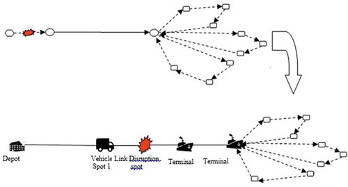
Figure 3. Disruption transformation process in case combinational disruption incident.

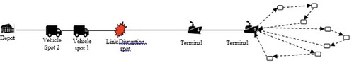
When two types of disruptions, namely link disruptions and customer disruptions, disrupt the network, the transformation process in the recovery model adds three kinds of new nodes as virtual nodes: namely, the link disruption spot node, vehicle spot 1 node, and vehicle spot 2 node. The link disruption spot node is used to accommodate the location of the disruption. Vehicle spot 1 nodes are used to accommodate the spot where the trucks in the original plan from the depot face the congestion that comes from the disruption node. Vehicle spot 2 nodes are used to accommodate the spot where the additional trucks from the depot in recovery plan face the congestion that comes from the disruption node. The location of this spot can be calculated using the concept of relative speed. From this concept, the time of the truck leaving the depot until it meets the congestion at the vehicle spot 1 node can be calculated. This condition is explained in Equation 23(23) $T{M}_{lkc}=Dis{t}_{ij}/v_k+v_{c}fori=\left\{0\right\},\mathrm{l}=\left\{1\right\},\mathrm{j}=\left\{2\right\},k\in K,m\in M$(23) . From that time, the distance between both nodes can be calculated using Equation 24(24) $Dis{t}_{lj}=T{M}_{ljkm}x{v}_{k}fori=\left\{1\right\},\mathrm{j}=\left\{3\right\},k\in K,m\in M$(24) .

(23) $T{M}_{lkc}=Dis{t}_{ij}/v_k+v_{c}fori=\left\{0\right\},\mathrm{l}=\left\{1\right\},\mathrm{j}=\left\{2\right\},k\in K,m\in M$(23)

(24) $Dis{t}_{lj}=T{M}_{ljkm}x{v}_{k}fori=\left\{1\right\},\mathrm{j}=\left\{3\right\},k\in K,m\in M$(24)

In this study, the average vehicle speed and the average of the congestion rate are known. The increase in travel time is calculated using an equation adopted from Rosyida et al. (2019).

3.2.3. Optimal starting time strategy for vehicles

Optimizing the starting time is a strategy for determining the departure time of trucks from each node. This optimization will reduce the total shipping costs when facing the time window limit of each node because every truck has the possibility for early, on time or late arrival(Wang et al., 2012). With various types of disruptions that may occur in the shipping path, this strategy is beneficial. The congestion factors influence the process of determining the optimal time. The formula for determining the optimal starting time is as follows:

(25) $\mathrm{T}\mathrm{D}\mathrm{\_}\mathrm{o}\mathrm{p}{\mathrm{t}}_{\mathrm{i}\mathrm{k}\mathrm{m}}=max\left(min\left({\mathrm{T}\mathrm{c}}_{\mathrm{m}\mathrm{t}}^{\mathrm{i}},{\mathrm{T}\mathrm{c}}_{\mathrm{m}\mathrm{t}}^{\mathrm{j}}-{\mathrm{T}}_{\mathrm{i}\mathrm{j}\mathrm{k}\mathrm{m}}\ast \mathrm{v}\right),{\mathrm{T}\mathrm{o}}_{\mathrm{m}\mathrm{t}}^{\mathrm{i}}\right)\mathrm{f}\mathrm{o}\mathrm{r}\mathrm{i}=\left\{0\right\},\mathrm{j}=\left\{1\right\},\mathrm{k}\in \mathrm{K},\mathrm{m}\in \mathrm{M}$(25)

The equation above explains the formula of the optimal departure time at node 1.

3.3. Recovery model

In the recovery model, some model notations change. The changes include the variable index and some newly added variables. All of the changing are explained below:

Table

$N_1$	Set of terminal node, $N_1$= {1 +b +a, 2 +b +a, … …, c +b +a}
$N_2$	Set of customer node, $N_2$ = {1 +c +b +a, 2 +c +b +a, … … d +c +b +a}
$N_3$	Set of disruption virtual node, $N_3$= {1}
$N_4$	Set of vehicle spot virtual node, $N_4$ = {2,3, … … .,a}
$N_5$	Set of vehicle spot virtual node, $N_5$ = {1 +a, 2 +a, … … b +a}
$N_o$	Set of all node (depot, terminal, customer, virtual node), $N_0=\left\{0\right\}{\cup }^{N_1}{\cup }^{N_2}{\cup }^{N_3}{\cup }^{N_4}{\cup }^{N_5}$

According to the explanation in the previous subsection, the recovery model is formulated as follows:

3.3.1. Objective function

(26) $\begin{array}{rl}& minZ={\sum }_{\left(i,j\right)\in N_o,k\in K,m\in M}{c}_{ijkm}{X}_{ijkm}+{\sum }_{\left(i,j\right)\in N_o,k\in K,m\in M}\left(0,3c_{ijkm}{X}_{ijkm}\right)+\\ & \left(0,7c_{ijkm}{X}_{ijkm}\right)(1-lw{d}_{jkm})+\left(c_{ijkm}{X}_{ijkm}+c_{ijkm}{X}_{ijkm}\right)lw{d}_{jkm}+{\sum }_{j\in N,k\in K}{\delta }_{jk}{\theta }_{jk}+\\ & {\sum }_{j\in N,k\in K,m\in M}{\beta }_{1}e{w}_{jkm}+{\beta }_{2}l{w}_{jkm}\end{array}$(26)

3.3.2. Flow constraint

(27) ${\sum }_{k\in K,m\in M}{U}_{ikm}=fori\in N_2$(27)

(28) ${\sum }_{k\in K,m\in M}{U}_{ikm}=1fori\in N_4$(28)

(29) ${\sum }_{k\in K,m\in M}{U}_{ikm}\le 1fori\in N_5$(29)

(30) ${\sum }_{k\in K,m\in M}{U}_{ikm}\le Kfori\in \left\{0\right\}{\cup }^{N_1}{\cup }^{N_3}$(30)

(31) ${\sum }_{j=1}^{Vc}{\sum }_{k=1}^K{\sum }_{m=1}^M{X}_{0jkm}={\sum }_{i=1}^{Vc}{\sum }_{k=1}^K{\sum }_{m=1}^M{X}_{i7km}\le K$(31)

(32) ${\sum }_{j=4}^{NewVc}{\sum }_{k=1}^K{\sum }_{m=1}^M{X}_{0jkm}={\sum }_{i=4}^{NewVc}{\sum }_{k=1}^K{\sum }_{m=1}^M{X}_{i7km}\le K$(32)

(33) ${\sum }_{l-0,l\ne i}^N{X}_{likm}={\sum }_{j-0,j\ne i}^N{X}_{ijkm}=U_{ikm}forN=N_0,k\in K,m\in M$(33)

(34) ${\sum }_{j=10}^N{\sum }_{k=1}^K{\sum }_{m=1}^M{X}_{9jkm}={\sum }_{i=10}^N{\sum }_{k=1}^K{\sum }_{m=1}^M{X}_{i9km}\le K$(34)

(35) ${\delta }_{jkm}\ge {\sum }_{i\in N_1{\cup }^{N_2}}{X}_{ijkm}-{\sum }_{i\in N_1{\cup }^{N_2}}{X}_{jikm}fork\in K,j\in N_1{\cup }^{N_2},m\in M$(35)

3.3.3. Capacity constraint

(36) $\sum _{i=1}^{N_2}{d}_i\times U_{ikm}\le q_{k}fork\in K,m=\left\{1\right\}$(36)

3.3.4. Delivery time constraint

(37) $T{A}_{jkm}\ge T{A}_{ikm}+se{r}_{ikm}+T_{ijkm}-\left(1-X_{ijkm}\right)xMfori=\left\{0,1,2,3,4,5,6,7\right\},j=[1,2,3,4,5,6,7,8\},k\in K,m=\left\{1\right\}$(37)

(38) $T{D}_{jkm}-\tau -T{A}_{jkm}+\left(M\ast lw{d}_{jkm}^2\right)forj=\left\{8\right\},k\in K,m\in M$(38)

(39) $T{D}_{jkm}\ge TDpla{n}_{jkm}+\left(\xi \ast lw{d}_{jkm}^2\right)forj=\left\{8\right\},k\in K,m\in M$(39)

(40) $E{W}_{jkm}\ge \left(T{o}_{mt}^j+\xi \left(t-1\right)\right)\ast U_{ikm}-\left(T{D}_{ikm}+T_{ijkm}\right)fori=\left\{7\right\},j=\left\{8\right\},k\in K,m\in M$(40)

(41) $E{W}_{jkm}\ge 0forj=\left\{8\right\},\mathrm{\forall }k\in K,m=\left\{2\right\}$(41)

(42) $L{W}_{jkm}\ge \left(T{o}_{mt+1}^j+\xi \right)\ast lw{d}_{jkm}^1-\left(T{D}_{ikm}+T_{ijkm}\right)fori=\left\{7\right\},j=\left\{8\right\},k\in K,m\in M$(42)

(43) $T{c}_{mt}^j-\left(T{D}_{ikm}+T_{ijkm}\right)+M\ast lw{d}_{jkm}^1\ge 0fori=\left\{8\right\},j=\left\{9\right\},k\in K,m\in M$(43)

(44) $L{W}_{jkm}\ge 0forj=\left\{8\right\},\mathrm{\forall }k\in K,m=\left\{2\right\}$(44)

(45) $\left(T{c}_{mt+1}^j+\xi \right)\ge \left(T{D}_{ikm}+T_{ijkm}\right)fori=\left\{7\right\},j=\left\{8\right\},k\in K,m\in M$(45)

(46) $lw{d}_{jkm}^1=\left\{1,0\right\}forj=\left\{8\right\},k\in K,m=\left\{2\right\}$(46)

(47) $T{A}_{jkm}\ge T{D}_{ikm}+se{r}_{ikm}+T_{ijkm}-\left(1-X_{ijkm}\right)xMfori=\left\{8\right\},j=[9\},k\in K,m=\left\{2\right\}$(47)

(48) $T{A}_{jkm}\ge T{A}_{ikm}+se{r}_{ikm}+T_{ijkm}-\left(1-X_{ijkm}\right)xMfori,j\in \left\{9,N_2\right\},k\in K,m\in M$(48)

(49) $T{A}_{jkm}\le Tre{q}_{jkm}\ast u_{jkm}fori,j\in N_2,k\in K,m\in M$(49)

(50) $X_{ijkm},U_{ikm},{\delta }_{jkm},lw{d}_{jkm}^2\in \left\{0,1\right\}$(50)

(51) $T{A}_{jkm}^{\hspace{0.17em}},T{D}_{ikm}^{\hspace{0.17em}}\ge 0$(51)

The objective function of this recovery model is to minimize the total cost. There are some new constraints and some alterations in constraints to accommodate the newly added nodes in the recovery model. Constraints (27) and (28) ensure that each customer is served only once and that each virtual vehicle node is visited by one and only one vehicle. Constraint (29) ensures that each virtual new vehicle node is visited by only one new vehicle or it is not visited. Constraint (30) ensures that the number of vehicles that leave from the depot and enter a virtual disruption node then enter the terminal should not exceed the total number of vehicles. Constraints (31) and (32) ensure that each vehicle should leave from the depot and enter into the terminal, and the total number of vehicles should not exceed the total number of vehicles on the depot. The rest of the constraints are the same as the constraints in the original model.

4. Methodology

The model developed is a complex combination case. The optimization procedure for complex cases is believed by some researchers to be inefficient when using analytic (exact) methods. A more efficient alternative approach is the metaheuristic. The metaheuristic approach used in this paper are the Genetic Algorithm (GA) and Simulated Annealing (SA). Both approaches can help achieve the optimal solution or close to the optimal with a faster time than the exact method such as the branch and bound.

The steps to find a solution are explained in Figure 4. The discovery of the solution begins with the development of an intermodal freight routing planning problem (IFRPP) model. Then, we developed the recovery model. Finding the solution is the next step. This step consists of 1) the clustering process, which is grouping customers based on the average distance between customers. Customer grouping results are converted into one shipping route where the order must match the group’s sequence. 2) This route sequence is for the input of GA and SA. This procedure is carried out because the initial good population as input for GA and SA will accelerate the achievement of optimal or near-optimal solutions.

The next step is finding solutions using GA and SA in two different cases. First, a simple case for model validation. The numerical test results are compared to those of the exact optimization method using Lingo software. If the results are not yet valid, a better solution finding process is needed. After the results are considered valid, the next optimization process is applying to complex cases where the data used are taken from Wang et al. (2012) that discusses VRP cases. The data is modified and adjusted to fit with real conditions based on several papers (Behdani et al., 2016; Widjanarka et al., 2018) and expert judgment. The procedure for each stage of finding the optimal value, which includes disruption transformation, clustering, GA and SA, and starting service time, will be discussed in more detail in the next sub-chapter.

Figure 4. The solution methodology.

4.1. Disruptions transformation

Disruption transformation aims to convert the disruption into the model. The process consists of adding several new nodes that consist of virtual nodes or new real nodes. The results of combining these nodes are used as the input of the recovery model. The disruptions discussed in this paper are link and customer disruptions. The transformation process for two types of disruptions are different, and the steps are as follows:

1. Link disruptions

The transformation steps are:

1. Set the initial x that consist of some node. The node consists of the depot, terminal, and some customer node.

2. Set the coordinate location of disruption as a disruption virtual node.

3. Set the coordinate location of the vehicle when the disruption occurs as a vehicle virtual node.

4. Calculate the distance between coordinate location in step b with the meet point between the coordinate location of step b and c as a second vehicle virtual node.

5. Add the virtual node in steps b, c, and d as a new member of x.

• (2) Customer disruptions

1. Set the initial x that consist of some node. The node consists of the depot, terminal, and some customer node.

2. Set the customer disruptions data.

3. Set the coordinate location of the vehicle when the disruption occurs as a vehicle virtual node.

4. Evaluate the shipment process. Separate the customer that has been served with unserved.

5. Transform the disruption with set the customer node. The steps are:

   1. For the additional demand disruption, the first way is to set the new ID for customer “n” with the same data of that customer “n” except the number of demand. The sum of the demand for this new customer is the number of additional requests.

   2. For the additional demand, and delivery location and time window changing, the way to transform is to set the new customer ID with the data changing. Then, we should remove the previous customer

   3. For delivery location and time window changing, the way to transform is to set the new customer ID with the change data submitted. The demand data is the same as the data before. Then, we should remove the previous customer.

   4. For the new customer request, set the new customer ID with their data.

   5. If there is an addition of new vehicle assignments, the vehicle location’s initial set at the depot and the departure of the new vehicle is the sum of the time of disruption and service time at the depot.

6. Add the member of x with the vehicle virtual node and new customer node. Then, delete customer data according to step-d.

• (3) Combinational Disruptions

1. Set the initial x that consist of some node. The node consists of the depot, terminal, and some customer node.

2. Set the combination of disruption data.

3. Set the coordinate location of disruption as a disruption virtual node.

4. Set the coordinate location of the vehicle when the disruption occurs as a vehicle virtual node and evaluate the shipment progress. List the customer that has been serviced and not been serviced yet.

5. Calculate the distance between the coordinate location in step c with the meeting point between the coordinate location of steps c and d as a second vehicle virtual node.

6. Transformed the customer disruptions with set the customer node. The steps use the customer disruptions step e.

7. Add the member of x with virtual disruption node, virtual vehicle node, and new customer node. Then, delete customer data according to step d.

4.2. Clustering

At this stage the cluster method is carried out twice, the first is grouping the intermodal transportation network into two groups, the first is the depots up to terminals 1 and 2. Next is terminal 2 and customers. For the first group, the route’s sequence is not as complicated as starting from the depot, terminal 1 and terminal 2. Whereas, for the second group, the series of tours are based on cluster results. The cluster is a customer cluster based on the distance between customers. The number of these clusters is the result of rounding the quotient of total customer demand with the truck capacity. This clustering process uses the K-means algorithm. The results of this clustering process are used as initial solutions for the next process, namely finding solutions with GA and SA.

4.3. The Genetic Algorithm (GA)

The main parameters of GA are population size, crossover probability, and mutation probability. In this study, GA parameters are based on route determination. One of these parameters is the number of customers (nodes) of the route. Generally, basic GA can be explained as follows (Santosa & Jin Ai, 2017):

1. Generating an initial population with certain size randomly.

2. Choose the best individual to be copied to replace a certain number of other individual (elitism)

3. Perform competitive selection to select members of the population as a parent to do crossover

4. Make crossover between parents selected to get a better combination between one individual with another in a population.

5. Choose a few individuals in the population to undergo a process of mutation.

4.4. The Simulated Annealing (SA)

The main parameters of SA are temperature (T) and temperature damping rate (c). The other parameter is the number of customers (nodes) of the route. The basic SA adopted from Santosa and Jin Ai (2017) with the following steps:

1. Generate an initial population with certain size randomly.

2. Choose the best individual to be the best fitness.

3. Generate the new individual in the vicinity with a current solution either with slip, swap and slide step.

4. Choose the best fitness between the best fitness in step 2 with the current fitness from the new individual or choose an even worse fitness using Metropolis Criteria.

4.5. Disrupted path length

The new point coordinate is the meeting location between the vehicles with the disruption. The purpose of determining this point is to estimate the total travel time when the trip delayed due to the disruption. The total travel time is calculated from the estimated congestion length, the distance between the initial location of the disruption and the coordinates of this new point is divided by the average speed of the vehicle. The stages are:

1. Set the location point of the initial disruption and vehicle location point when the disruption occurs.

2. Calculate the distance between the two points in step a.

3. Set the average vehicle speed and disruption rate.

4. Calculate the predicted passage of time between the vehicle and the disruption using Equation 23(23) $T{M}_{lkc}=Dis{t}_{ij}/v_k+v_{c}fori=\left\{0\right\},\mathrm{l}=\left\{1\right\},\mathrm{j}=\left\{2\right\},k\in K,m\in M$(23) .

5. Calculate the distance between the initial location of the disruption and the site where the disturbance has met the vehicle using Equation 24(24) $Dis{t}_{lj}=T{M}_{ljkm}x{v}_{k}fori=\left\{1\right\},\mathrm{j}=\left\{3\right\},k\in K,m\in M$(24) .

6. Calculate the predicted length of the disrupted path by converting this distance by considering the congestion factor (Rosyida et al., 2019). The total time is obtained by dividing the distance with the average vehicle speed.

4.6. Starting service time

The starting service time optimization is calculated to estimate the depot’s vehicle departure time so that it does not experience delays at the terminal. The stages of determining the time are:

1. Set the depot coordinates and terminal nodes, depot and terminal time windows, and

2. Service time at nodes and terminals.

3. Calculate the total travel time from the depot to the terminal.

4. Set the congestion factor (v).

5. Calculate the optimal departure time from a depot using Equation 25(25) $\mathrm{T}\mathrm{D}\mathrm{\_}\mathrm{o}\mathrm{p}{\mathrm{t}}_{\mathrm{i}\mathrm{k}\mathrm{m}}=max\left(min\left({\mathrm{T}\mathrm{c}}_{\mathrm{m}\mathrm{t}}^{\mathrm{i}},{\mathrm{T}\mathrm{c}}_{\mathrm{m}\mathrm{t}}^{\mathrm{j}}-{\mathrm{T}}_{\mathrm{i}\mathrm{j}\mathrm{k}\mathrm{m}}\ast \mathrm{v}\right),{\mathrm{T}\mathrm{o}}_{\mathrm{m}\mathrm{t}}^{\mathrm{i}}\right)\mathrm{f}\mathrm{o}\mathrm{r}\mathrm{i}=\left\{0\right\},\mathrm{j}=\left\{1\right\},\mathrm{k}\in \mathrm{K},\mathrm{m}\in \mathrm{M}$(25) .

5. Numerical experiment

The system used in this paper consists of eighteen nodes: one node as the depot, two-node as the terminals, and fifteen nodes as the customers. The sources of data in this numerical experiment are published papers and real conditions. The coordinate node, customer demand, cost, and time window are obtained from published papers, namely Wang et al. (2012), Behdani et al. (2016), and Widjanarka et al. (2018). The transportation costs are 1 USD/km for trucks and the cost for a ship is explained in the next paragraph. The capacity for each container is 6.5. The speed of each truck is 60 km/hour.

On the other hand, the terminal time window data is adopted from several journals that discussed the time appointment system (TAS). The TAS topic is used to analyze the optimal time window in the terminal. Some papers analyze terminal profits and some other papers analyze profits both at the terminal and truck companies (freight forwarders). Besides, some papers also analyze the emissions. The terminal time windows for every truck are different. They depend on the original contract between the terminal operator and freight forwarder. The terminal operator gives a time window option, the freight forwarder selects an option, and then the terminal operator agrees if the capacity in that period is still available and switches to another period if it is full.

The average range of time window periods studied varies from 1 to 3 hours, where the time window is the terminal operating hours. Time window appointments are determined within a range of 3 hours, and there are two time window periods, namely 06.00–09.00 and 09.00–12.00. Terminal operation hours are 24 hours per day. If the truck does not arrive according to the agreed time window, the truck will be penalized 1 USD per unit time window if it arrives before the opening time and 4 USD per unit time window if it arrives after the closing time. The maximum limit for trucks entering the terminal is 6 hours before the ship’s departure. If the truck arrives after the time limit, it is assumed that the truck cannot use the capacity booked and the truck must wait for the departure of the next ship. In this condition, the capacity booking fee is assumed to be lost and the freight forwarder must buy the capacity with “on the spot” type cost. There are two payment models when using ship capacity: buy with a booking fee and buy on the spot. The cost of transportation using the ship mode is 700 USD per-container with a booking fee of 210 USD and an additional capacity will be charged 1050 USD per TEU (Widjanarka et al., 2018). The ship’s departure time is 24 hours. The departure time of the container at the depot node is assumed to be 0 hours. The terminal transfer cost is 65 USD (Ishfaq, 2012) and 3 hours are spent on transferring in terminal (Behdani et al., 2016).

The purpose of this numerical experiment is to analyze the impact of the disruptions on the shipping cost. Numerical experiments are carried out on simple and complex cases. In a simple case, we use the exact optimization to solve the problem. As for complex cases, exact optimization methods are less efficient when used. As described in Figure 3, for a simple case, three different optimization approaches namely the exact optimization, GA, and SA. These results will give a hint that the recovery model developed is feasible to use. Besides, the comparison of results can be used to conclude that the two metaheuristics are appropriate to solve complex cases when the exact optimization method is less efficient to use.

The main parameters used in the GA and SA are presented in Table 2. Furthermore, all algorithms coded using the Lingo 18 and the MATLAB R2019b-academic use software.

Table 1. Coordinate node, customer demand, and customer time windows

Node	Coordinate		Demand	To	Tc
	x	Y
0	400	400
term 1	325	325
term 2	90	95
cust 1	19	90	1	41	60
cust 2	33	75	1.8	40	62
cust 3	20	60	1.1	25	55
cust 4	53	19	0.6	21	50
cust 5	140	94	1.9	40	56
cust 6	27	44	1.4	41	60
cust 7	75	140	1.2	21	60
cust 8	56	4	0.2	24	55
cust 9	30	120	1.7	30	55
cust 10	120	76	0.8	21	56
cust 11	41	50	0.9	32	60
cust 12	83	43	0.8	32	66
cust 13	40	110	1.9	30	60
cust 14	73	29	1.6	20	45
cust 15	70	18	0.9	41	62

Table 2. The parameter of GA and SA

GA	SA
P_Crossover =0,8 P_mutation = 0,5 Population = 10 Stopping Criteria = 1000 iteration	Initial Temperature = 100 Temperature Damping Rate = 0,5 Stopping Criteria = 1000 iteration

5.1. The disruptions

The link disruptions considered are disruptions that occur in a roadway that makes the average speed of vehicles decrease, which then causes congestion. A scenario of 10 levels of the average vehicle speed is adopted from Pregnolato et al. (2017). Pregnolato et al. (2017) designed the average speed level of the vehicle based on the depth of a puddle caused by the high rainfall that occurred. The data is presented in Table 3. The disruption location is at coordinates [360,360], and the vehicle faces the disruption impact at coordinates [340,340]. Meanwhile, the second disruption is the customer disruption. This disruption includes changes in the demand number, customer time window, and changes in shipping locations. Some of the changing data are adopted from Wang et al. (2012) and presented in Table 4.

Table 3. Vehicle speed scenario

Speed (Km/Hour)
60	50	45	37	26	24	16	7	3	0

Table 4. The Changing Data of Customer Demand, Customer Time Window and Customer Location

New Data	Customer
	4	8	11	14	16
Coordinates	(53,29)	-	-	-	(55,60)
Time Window	[38 62]	-	-	[37 55]	[30 61]
Demand	1.6	1.4	1.9	-	2

The numerical test scenario is based on a combination of disruptions. In the first scenario, only one disruption is tried. The next scenario is a combination of disruptions, disruptions in Scenario 1 and customer disruptions. The scenario is as follows:

1. Link Disruption.

2. The combination of disruptions in scenario number 1 with customer disruptions.

3. The disruptions scenarios analyzed with two conditions considered; 1. Considering the starting time optimization strategy; 2. Without considering the starting time strategy at number 1.

4. The next scenario is related to the choice of the carrier capacity usage system at the port (30% first and purchase on the spot). Disruption scenarios, starting time, optimization strategy scenarios as well as contract selection strategies for using carrier capacity at the port are combined to get the optimal system conditions.

5.2. The disruption transformation

Disruption transformations are performed on disrupted nodes and links. For a disrupted link, three new points are created as virtual nodes. The locations of the virtual nodes are between the depot and terminal 1. The virtual nodes include a virtual disruption node, some virtual in-transit vehicle nodes, and some virtual new in-transit vehicle nodes. The coordinate location of the virtual disruption node is [360,360], and [340,340] is the coordinate for the virtual in-transit vehicle node. Node 7 is a virtual disruption node, a new node that is transformed from link disruptions and becomes a starting point for the average speed level of a vehicle to change. Nodes 1, 2, and 3 are virtual in-transit vehicle nodes. These nodes serve as the bound spot of the average speed level change from node 7 and accommodate the vehicle that is dispatched in the original plan. The coordinates of the virtual new in-transit vehicle nodes are calculated using Equations (23)(23) $T{M}_{lkc}=Dis{t}_{ij}/v_k+v_{c}fori=\left\{0\right\},\mathrm{l}=\left\{1\right\},\mathrm{j}=\left\{2\right\},k\in K,m\in M$(23) and (24(24) $Dis{t}_{lj}=T{M}_{ljkm}x{v}_{k}fori=\left\{1\right\},\mathrm{j}=\left\{3\right\},k\in K,m\in M$(24) ). These virtual nodes accommodate the new vehicle that is dispatched in the recovery model. From this coordinate, the distance between the disruption node and this node itself is calculated. Then, the perceived length of that link is calculated to analyze the increase in total time travel.

In customer disruption, as presented in Table 4, five disruptions came from the customers: 4, 8, 11, 14, and new requests as the last customer disruption. The transformations are done by transforming the disruptions into three virtual customers and adding five new customer nodes (customers 16, 17, 18, 19, and 20). Three virtual customers are the same as the virtual in-transit vehicle nodes. New events are from customer 8 to customer 18 and node customer 11 to customer 19; while for old events, they remain the same with customers 8 and 11. On the other hand, request changes in the customer 4 and 14 nodes are transformed into customers 16 and 17 nodes, respectively, while customer 4 and 14 nodes are removed. Then, customer 20 is a new request.

5.3. Model validation

The validation process used a portion of data from the system that includes a depot, two terminals, and the first four customers presented in Table 1. The type of disruptions and the disruptions transformation process are described in the previous sub-chapter. For the simple case, the disruptions and transformation process data used are only for the first four customers, depot and terminal nodes.

The numerical test results are presented in Tables 5-7. Table 5 shows the IFRPP optimization results with the simple case. Table 6 presents the optimization of the IFRPP recovery model considering the link disruptions. In addition, Table 7 explains the optimization of the IFRPP recovery model considering the combinational interruptions. The test results include the best route, the shipment total cost, and the time status of each vehicle when entering the terminal, either on-time or coming too early or too late. The three optimization methods show similar results from all outcome criteria. These results mean that the GA and SA approaches could optimize the IFRPP recovery model.

Table 5. The IFRPP optimization result with simple case

Methods	The Routings	Total Cost ($)	*Number of Vehicle
			on time	early arrival	late
Up_front_fee strategy without consider starting time optimization
Exact method	[d,t1,t2,c1,c2,t2],[d-t1,t2,c3,c4,t2]	2282.6	0	2	0
Genetic Algorithm	[d,t1,t2,c1,c2,t2],[d-t1,t2,c3,c4,t2]	2282.6	0	2	0
Simulated Annealing	[d,t1,t2,c1,c2,t2],[d-t1,t2,c3,c4,t2]	2282.6	0	2	0
Up_front_fee strategy with consider starting time optimization
Exact method	[d,t1,t2,c1,c2,t2],[d-t1,t2,c3,c4,t2]	2282.6	2	0	0
Genetic Algorithm	[d,t1,t2,c1,c2,t2],[d-t1,t2,c3,c4,t2]	2282.6	2	0	0
Simulated Annealing	[d,t1,t2,c1,c2,t2],[d-t1,t2,c3,c4,t2]	2282.6	2	0	0
On_the_spot strategy without consider starting time optimization
Exact method	[d,t1,t2,c1,c2,t2],[d-t1,t2,c3,c4,t2]	3052.2	0	2	0
Genetic Algorithm	[d,t1,t2,c1,c2,t2],[d-t1,t2,c3,c4,t2]	3052.2	0	2	0
Simulated Annealing	[d,t1,t2,c1,c2,t2],[d-t1,t2,c3,c4,t2]	3052.2	0	2	0
On_the_spot strategy with consider starting time optimization
Exact method	[d,t1,t2,c1,c2,t2],[d-t1,t2,c3,c4,t2]	3052.2	2	0	0
Genetic Algorithm	[d,t1,t2,c1,c2,t2],[d-t1,t2,c3,c4,t2]	3052.2	2	0	0
Simulated Annealing	[d,t1,t2,c1,c2,t2],[d-t1,t2,c3,c4,t2]	3052.2	2	0	0

Table 6. The RIFRPP optimization result with simple case considering link disruptions

Methods	The Routings	Total Cost ($)		*Number of Vehicle
		45	3	on time		early arrival		late
				45	3	45	3	45	3
Up_front_fee strategy without consider starting time optimization
Exact method	[d,vt1,vtd1,vd,t1,t2,c2,c1,t2],[d, vt2,vtd2,vd,t1,t2,c3,c4,t2]	2387.2	5473.1	0	2	2	0	0	0
Genetic Algorithm	[d,vt1,vtd1,vd,t1,t2,c2,c1,t2],[d, vt2,vtd2,vd,t1,t2,c3,c4,t2]	2387.2	5473.1	0	2	2	0	0	0
Simulated Annealing	[d,vt1,vtd1,vd,t1,t2,c2,c1,t2],[d, vt2,vtd2,vd,t1,t2,c3,c4,t2]	2387.2	5473.1	0	2	2	0	0	0
Up_front_fee strategy with consider starting time optimization
Exact method	[d,vt1,vtd1,vd,t1,t2,c2,c1,t2],[d, vt2,vtd2,vd,t1,t2,c3,c4,t2]	2385.2	5473.1	2	2	0	0	0	0
Genetic Algorithm	[d,vt1,vtd1,vd,t1,t2,c2,c1,t2],[d, vt2,vtd2,vd,t1,t2,c3,c4,t2]	2385.2	5473.1	2	2	0	0	0	0
Simulated Annealing	[d,vt1,vtd1,vd,t1,t2,c2,c1,t2],[d, vt2,vtd2,vd,t1,t2,c3,c4,t2]	2385.2	5473.1	2	2	0	0	0	0
On_the_spot strategy without consider starting time optimization
Exact method	[d,vt1,vtd1,vd,t1,t2,c2,c1,t2],[d, vt2,vtd2,vd,t1,t2,c3,c4,t2]	3087.2	4965.1	0	2	2	0	0	0
Genetic Algorithm	[d,vt1,vtd1,vd,t1,t2,c2,c1,t2],[d, vt2,vtd2,vd,t1,t2,c3,c4,t2]	3087.2	4965.1	0	2	2	0	0	0
Simulated Annealing	[d,vt1,vtd1,vd,t1,t2,c2,c1,t2],[d, vt2,vtd2,vd,t1,t2,c3,c4,t2]	3087.2	4965.1	0	2	2	0	0	0
On_the_spot strategy with consider starting time optimization
Exact method	[d,vt1,vtd1,vd,t1,t2,c2,c1,t2],[d, vt2,vtd2,vd,t1,t2,c3,c4,t2]	3085.2	4965.1	2	2	0	0	0	0
Genetic Algorithm	[d,vt1,vtd1,vd,t1,t2,c2,c1,t2],[d, vt2,vtd2,vd,t1,t2,c3,c4,t2]	3085.2	4965.1	2	2	0	0	0	0
Simulated Annealing	[d,vt1,vtd1,vd,t1,t2,c2,c1,t2],[d, vt2,vtd2,vd,t1,t2,c3,c4,t2]	3085.2	4965.1	2	2	0	0	0	0

Table 7. The RIFRPP optimization result with simple case considering combinational disruptions

Methods	The Routings	Total Cost ($)		*Number of Vehicle
				on time		early arrival		late
		45	3	45	3	45	3	45	3
Up_front_fee strategy without consider starting time optimization
Exact method	[d,vt1,vtd1,vd,t1,t2,c5,c4,t2],[d,vt2,vtd2,vd,t1,t2,c1,c3,t2],[d,vtd3,vd,t1,t2,c2,t2]	3498.1	7995	0	2	3	0	0	1
Genetic Algorithm	[d,vt1,vtd1,vd,t1,t2,c5,c4,t2],[d,vt2,vtd2,vd,t1,t2,c1,c3,t2],[d,vtd3,vd,t1,t2,c2,t2]	3498.1	7995	0	2	3	0	0	1
Simulated Annealing	[d,vt1,vtd1,vd,t1,t2,c5,c4,t2],[d,vt2,vtd2,vd,t1,t2,c1,c3,t2],[d,vtd3,vd,t1,t2,c2,t2]	3498.1	7995	0	2	3	0	0	1
Up_front_fee strategy with consider starting time optimization
Exact method	[d,vt1,vtd1,vd,t1,t2,c5,c4,t2],[d,vt2,vtd2,vd,t1,t2,c1,c3,t2],[d,vtd3,vd,t1,t2,c2,t2]	3495.1	7995	3	2	0	0	0	1
Genetic Algorithm	[d,vt1,vtd1,vd,t1,t2,c5,c4,t2],[d,vt2,vtd2,vd,t1,t2,c1,c3,t2],[d,vtd3,vd,t1,t2,c2,t2]	3495.1	7995	3	2	0	0	0	1
Simulated Annealing	[d,vt1,vtd1,vd,t1,t2,c5,c4,t2],[d,vt2,vtd2,vd,t1,t2,c1,c3,t2],[d,vtd3,vd,t1,t2,c2,t2]	3495.1	7995	3	2	0	0	0	1
On_the_spot strategy without consider starting time optimization
Exact method	[d,vt1,vtd1,vd,t1,t2,c5,c4,t2],[d,vt2,vtd2,vd,t1,t2,c1,c3,t2],[d,vtd3,vd,t1,t2,c2,t2]	4548.1	6426.1	0	2	3	0	0	1
Genetic Algorithm	[d,vt1,vtd1,vd,t1,t2,c5,c4,t2],[d,vt2,vtd2,vd,t1,t2,c1,c3,t2],[d,vtd3,vd,t1,t2,c2,t2]	4548.1	6426.1	0	2	3	0	0	1
Simulated Annealing	[d,vt1,vtd1,vd,t1,t2,c5,c4,t2],[d,vt2,vtd2,vd,t1,t2,c1,c3,t2],[d,vtd3,vd,t1,t2,c2,t2]	4548.1	6426.1	0	2	3	0	0	1
On_the_spot strategy with consider starting time optimization
Exact method	[d,vt1,vtd1,vd,t1,t2,c5,c4,t2],[d,vt2,vtd2,vd,t1,t2,c1,c3,t2],[d,vtd3,vd,t1,t2,c2,t2]	4545.1	6426.1	3	2	0	0	0	1
Genetic Algorithm	[d,vt1,vtd1,vd,t1,t2,c5,c4,t2],[d,vt2,vtd2,vd,t1,t2,c1,c3,t2],[d,vtd3,vd,t1,t2,c2,t2]	4545.1	6426.1	3	2	0	0	0	1
Simulated Annealing	[d,vt1,vtd1,vd,t1,t2,c5,c4,t2],[d,vt2,vtd2,vd,t1,t2,c1,c3,t2],[d,vtd3,vd,t1,t2,c2,t2]	4545.1	6426.1	3	2	0	0	0	1

Tables 5 and 6 show that the optimal route without disruption is the same as the optimal route when the link disruption occurs. The difference between the two results lies in the total cost. The overall cost increases when a link disruption occurs. Meanwhile, Table 7 shows the optimal route results that are different from those of the previous scenario. There is an increase in the number of trucks assigned so that the route formed is three while the last route yield is two. Besides, the impact of combinational disruptions shown in Table 7 also included an increase in total costs when compared with the total expenses from the results of the previous scenario.

6. Results and discussion

The results of the numerical experiment for each scenario are summarized in Tables 8-11. Table 8 presents the results of the IFRPP optimization. Table 9 shows the results of the optimal routes for each scenario. While, Table 10 illustrates the results of IFRPP Recovery optimization considering link disruptions. In addition, the results of IFRPP Recovery optimization considering combinational disruptions are explained in Table 11.

Table 8. The I FRPP optimization result with complex case

Methods	The Routings	Total Cost ($)	*Number of Vehicle
			on time	early arrival	Late
Up_front_fee strategy without consider starting time optimization
Genetic Algorithm	[d,vt1,vtd1,vd,t1,t2,c8,c2,c1,c3,c11,c4,c15,t2] [d,vt2,vtd2,vd,t1,t2,c13,c9,c7,c6,t2] [d,vt3,vtd3,vd,t1,t2,c12,c14,c10,c5,t2]	3557.6	0	3	0
Simulated Annealing	[d,vt1,vtd1,vd,t1,t2,c15,c4,c8,c11,c2,c1,c4,t2] [d,vt2,vtd2,vd,t1,t2,c12,c14,c10,c5,t2] [d,vt3,vtd3,vd,t1,t2,c13,c9,c7,c6,t2]	3547.2	0	3	0
Up_front_fee strategy with consider starting time optimization
Genetic Algorithm	[d,vt1,vtd1,vd,t1,t2,c8,c2,c1,c3,c11,c4,c15,t2] [d,vt2,vtd2,vd,t1,t2,c13,c9,c7,c6,t2] [d,vt3,vtd3,vd,t1,t2,c12,c14,c10,c5,t2]	3554.6	3	0	0
Simulated Annealing	[d,vt1,vtd1,vd,t1,t2,c15,c4,c8,c11,c2,c1,c4,t2] [d,vt2,vtd2,vd,t1,t2,c12,c14,c10,c5,t2] [d,vt3,vtd3,vd,t1,t2,c13,c9,c7,c6,t2]	3544.2	3	0	0
On_the_spot strategy without consider starting time optimization
Genetic Algorithm	[d,vt1,vtd1,vd,t1,t2,c8,c2,c1,c3,c11,c4,c15,t2] [d,vt2,vtd2,vd,t1,t2,c13,c9,c7,c6,t2] [d,vt3,vtd3,vd,t1,t2,c12,c14,c10,c5,t2]	4607.6	0	3	0
Simulated Annealing	[d,vt1,vtd1,vd,t1,t2,c15,c4,c8,c11,c2,c1,c4,t2] [d,vt2,vtd2,vd,t1,t2,c12,c14,c10,c5,t2] [d,vt3,vtd3,vd,t1,t2,c13,c9,c7,c6,t2]	4597.2	0	3	0
On_the_spot strategy with consider starting time optimization
Genetic Algorithm	[d,vt1,vtd1,vd,t1,t2,c8,c2,c1,c3,c11,c4,c15,t2] [d,vt2,vtd2,vd,t1,t2,c13,c9,c7,c6,t2] [d,vt3,vtd3,vd,t1,t2,c12,c14,c10,c5,t2]	4604.6	3	0	0
Simulated Annealing	[d,vt1,vtd1,vd,t1,t2,c15,c4,c8,c11,c2,c1,c4,t2] [d,vt2,vtd2,vd,t1,t2,c12,c14,c10,c5,t2] [d,vt3,vtd3,vd,t1,t2,c13,c9,c7,c6,t2]	4594.2	3	0	0

Table 9. The comparison of routing

Vehicle roadway speed	Method	Routing
		Without starting time strategy		starting time strategy
		upfront fee	on the spot	upfront fee	on the spot
Link Disruptions
7 s/d 60	GA	[d,vt1,vtd1,vd,t1,t2,c8,c2,c1,c3,c11,c4,c15,t2] [d,vt2,vtd2,vd,t1,t2,c13,c9,c7,c6,t2] [d,vt3,vtd3,vd,t1,t2,c12,c14,c10,c5,t2]	[d,vt1,vtd1,vd,t1,t2,c8,c2,c1,c3,c11,c4,c15,t2] [d,vt2,vtd2,vd,t1,t2,c13,c9,c7,c6,t2] [d,vt3,vtd3,vd,t1,t2,c12,c14,c10,c5,t2]	[d,vt1,vtd1,vd,t1,t2,c8,c2,c1,c3,c11,c4,c15,t2] [d,vt2,vtd2,vd,t1,t2,c13,c9,c7,c6,t2] [d,vt3,vtd3,vd,t1,t2,c12,c14,c10,c5,t2]	[d,vt1,vtd1,vd,t1,t2,c8,c2,c1,c3,c11,c4,c15,t2] [d,vt2,vtd2,vd,t1,t2,c13,c9,c7,c6,t2] [d,vt3,vtd3,vd,t1,t2,c12,c14,c10,c5,t2]
	SA	[d,vt1,vtd1,vd,t1,t2,c15,c4,c8,c11,c2,c1,c4,t2] [d,vt2,vtd2,vd,t1,t2,c12,c14,c10,c5,t2] [d,vt3,vtd3,vd,t1,t2,c13,c9,c7,c6,t2]	[d,vt1,vtd1,vd,t1,t2,c15,c4,c8,c11,c2,c1,c4,t2] [d,vt2,vtd2,vd,t1,t2,c12,c14,c10,c5,t2] [d,vt3,vtd3,vd,t1,t2,c13,c9,c7,c6,t2]	[d,vt1,vtd1,vd,t1,t2,c15,c4,c8,c11,c2,c1,c4,t2] [d,vt2,vtd2,vd,t1,t2,c12,c14,c10,c5,t2] [d,vt3,vtd3,vd,t1,t2,c13,c9,c7,c6,t2]	[d,vt1,vtd1,vd,t1,t2,c15,c4,c8,c11,c2,c1,c4,t2] [d,vt2,vtd2,vd,t1,t2,c12,c14,c10,c5,t2] [d,vt3,vtd3,vd,t1,t2,c13,c9,c7,c6,t2]
< 3	GA	[d,vt1,vtd1,vd,t1,t2,c8,c2,c1,t2] [d,vt2,vtd2,vd,t1,t2,c3,c11,c4,c15,t2] [d,vt3,vtd3,vd,t1,t2,c13,t2] [d,vtd4,vd,t1,t2,c9,c7,c6,c12,t2] [d,vtd5,vd,t1,t2,c5,t2]	[d,vt1,vtd1,vd,t1,t2,c8,c2,c1,t2] [d,vt2,vtd2,vd,t1,t2,c3,c11,c4,c15,t2] [d,vt3,vtd3,vd,t1,t2,c13,t2] [d,vtd4,vd,t1,t2,c9,c7,c6,c12,t2] [d,vtd5,vd,t1,t2,c5,t2]	[d,vt1,vtd1,vd,t1,t2,c8,c2,c1,t2] [d,vt2,vtd2,vd,t1,t2,c3,c11,c4,c15,t2] [d,vt3,vtd3,vd,t1,t2,c13,t2] [d,vtd4,vd,t1,t2,c9,c7,c6,c12,t2] [d,vtd5,vd,t1,t2,c5,t2]	[d,vt1,vtd1,vd,t1,t2,c8,c2,c1,t2] [d,vt2,vtd2,vd,t1,t2,c3,c11,c4,c15,t2] [d,vt3,vtd3,vd,t1,t2,c13,t2] [d,vtd4,vd,t1,t2,c9,c7,c6,c12,t2] [d,vtd5,vd,t1,t2,c5,t2]
	SA	[d,vt1,vtd1,vd,t1,t2,c8,c2,c1,c11,c4,c15,c12,t2] [d,vt2,vtd2,vd,t1,t2,c5,c9,c7,t2] [d,vt3,vtd3,vd,t1,t2,c10,c14,t2] [d,vtd4,vd,t1,t2,c3,c6,c13,t2]	[d,vt1,vtd1,vd,t1,t2,c8,c15,c13,t2] [d,vt2,vtd2,vd,t1,t2,c3,c1,c2,c11,c4,c12,t2] [d,vt3,vtd3,vd,t1,t2,c5,c9,c7,c6,t2] [d,vtd4,vd,t1,t2,c10,c14,t2]	[d,vt1,vtd1,vd,t1,t2,c8,c2,c1,c11,c4,c15,c12,t2] [d,vt2,vtd2,vd,t1,t2,c5,c9,c7,t2] [d,vt3,vtd3,vd,t1,t2,c10,c14,t2] [d,vtd4,vd,t1,t2,c3,c6,c13,t2]	[d,vt1,vtd1,vd,t1,t2,c8,c15,c13,t2] [d,vt2,vtd2,vd,t1,t2,c3,c1,c2,c11,c4,c12,t2] [d,vt3,vtd3,vd,t1,t2,c5,c9,c7,c6,t2] [d,vtd4,vd,t1,t2,c10,c14,t2]
Combinational Disruption
7 s/d 60	GA	[d,vt1,vtd1,vd,t1,t2,c16,c8,c18,c17,c15,c19,t2] [d,vt2,vtd2,vd,t1,t2,c20,c13,c1,c3,t2] [d,vt3,vtd3,vd,t1,t2,c9,c7,c5,c10,c12,t2] [d,vtd4,vd,t1,t2,c2,c6,c11,t2]	[d,vt1,vtd1,vd,t1,t2,c16,c8,c18,c17,c15,c19,t2] [d,vt2,vtd2,vd,t1,t2,c20,c13,c1,c3,t2] [d,vt3,vtd3,vd,t1,t2,c9,c7,c5,c10,c12,t2] [d,vtd4,vd,t1,t2,c2,c6,c11,t2]	[d,vt1,vtd1,vd,t1,t2,c16,c8,c18,c17,c15,c19,t2] [d,vt2,vtd2,vd,t1,t2,c20,c13,c1,c3,t2] [d,vt3,vtd3,vd,t1,t2,c9,c7,c5,c10,c12,t2] [d,vtd4,vd,t1,t2,c2,c6,c11,t2]	[d,vt1,vtd1,vd,t1,t2,c16,c8,c18,c17,c15,c19,t2] [d,vt2,vtd2,vd,t1,t2,c20,c13,c1,c3,t2] [d,vt3,vtd3,vd,t1,t2,c9,c7,c5,c10,c12,t2] [d,vtd4,vd,t1,t2,c2,c6,c11,t2]
	SA	[d,vt1,vtd1,vd,t1,t2,c16,c8,c18,c15,c17,c12,t2] [d,vt2,vtd2,vd,t1,t2,c6,c1,c2,c4,t2] [d,vt3,vtd3,vd,t1,t2,c20,c11,c19,c5,t2] [d,vtd4,vd,t1,t2,c13,c9,c7,c10,t2]	[d,vt1,vtd1,vd,t1,t2,c20,c6,c19,c11,c10,t2] [d,vt2,vtd2,vd,t1,t2,c3,c2,c1,c18,c8,c15,t2] [d,vt3,vtd3,vd,t1,t2,c5,c16,c17,c12,t2] [d,vtd4,vd,t1,t2,c13,c9,c7,t2]	[d,vt1,vtd1,vd,t1,t2,c16,c8,c18,c15,c17,c12,t2] [d,vt2,vtd2,vd,t1,t2,c6,c1,c2,c4,t2] [d,vt3,vtd3,vd,t1,t2,c20,c11,c19,c5,t2] [d,vtd4,vd,t1,t2,c13,c9,c7,c10,t2]	[d,vt1,vtd1,vd,t1,t2,c20,c6,c19,c11,c10,t2] [d,vt2,vtd2,vd,t1,t2,c3,c2,c1,c18,c8,c15,t2] [d,vt3,vtd3,vd,t1,t2,c5,c16,c17,c12,t2] [d,vtd4,vd,t1,t2,c13,c9,c7,t2]
< 3	GA	[d,vt1,vtd1,vd,t1,t2,c3,c2,c11,t2] [d,vt2,vtd2,vd,t1,t2,c9,t2] [d,vt3,vtd3,vd,t1,t2,c8,c15,c19,c13,t2] [d,vtd4,vd,t1,t2,c18,c20,c16,c6,t2] [d,vtd5,vd,t1,t2,c17,c10,t2] [d,vtd6,vd,t1,t2,c5,c12,c7,c1,t2]	[d,vt1,vtd1,vd,t1,t2,c9,c20,c1,c18,t2] [d,vt2,vtd2,vd,t1,t2,c10,t2] [d,vt3,vtd3,vd,t1,t2,c17,c6,c7,t2] [d,vtd4,vd,t1,t2,c5,c19,c12,c15,t2] [d,vtd5,vd,t1,t2,c8,c11,c13,t2] [d,vtd6,vd,t1,t2,c3,c16,c2,t2]	[d,vt1,vtd1,vd,t1,t2,c3,c2,c11,t2] [d,vt2,vtd2,vd,t1,t2,c9,t2] [d,vt3,vtd3,vd,t1,t2,c8,c15,c19,c13,t2] [d,vtd4,vd,t1,t2,c18,c20,c16,c6,t2] [d,vtd5,vd,t1,t2,c17,c10,t2] [d,vtd6,vd,t1,t2,c5,c12,c7,c1,t2]	[d,vt1,vtd1,vd,t1,t2,c9,c20,c1,c18,t2] [d,vt2,vtd2,vd,t1,t2,c10,t2] [d,vt3,vtd3,vd,t1,t2,c17,c6,c7,t2] [d,vtd4,vd,t1,t2,c5,c19,c12,c15,t2] [d,vtd5,vd,t1,t2,c8,c11,c13,t2] [d,vtd6,vd,t1,t2,c3,c16,c2,t2]
	SA	[d,vt1,vtd1,vd,t1,t2,c8,c18,c2,c1,c20,t2] [d,vt2,vtd2,vd,t1,t2,c10,c17,c15,c12,t2] [d,vt3,vtd3,vd,t1,t2,c5,t2] [d,vtd4,vd,t1,t2,c9,c7,c13,t2] [d,vtd5,vd,t1,t2,c3,c16,c6,c11,c19,t2]	[d,vt1,vtd1,vd,t1,t2,c3,c1,c2,c18,c15,t2] [d,vt2,vtd2,vd,t1,t2,c12,c17,t2] [d,vt3,vtd3,vd,t1,t2,c8,c16,c6,c11,c19,t2] [d,vtd4,vd,t1,t2,c9,c7,c13,t2] [d,vtd5,vd,t1,t2,c5,c10,c20,t2]	[d,vt1,vtd1,vd,t1,t2,c8,c18,c2,c1,c20,t2] [d,vt2,vtd2,vd,t1,t2,c10,c17,c15,c12,t2] [d,vt3,vtd3,vd,t1,t2,c5,t2] [d,vtd4,vd,t1,t2,c9,c7,c13,t2] [d,vtd5,vd,t1,t2,c3,c16,c6,c11,c19,t2]	[d,vt1,vtd1,vd,t1,t2,c3,c1,c2,c18,c15,t2] [d,vt2,vtd2,vd,t1,t2,c12,c17,t2] [d,vt3,vtd3,vd,t1,t2,c8,c16,c6,c11,c19,t2] [d,vtd4,vd,t1,t2,c9,c7,c13,t2] [d,vtd5,vd,t1,t2,c5,c10,c20,t2]

Table 10. The RIFRPP optimization result with simple case consider link disruptions

Methods	Up-Front Fee Strategy					On The Spot Strategy
	Speed Scenario	Total Cost ($)	*Number of Vehicle			Speed Scenario	Total Cost ($)	*Number of Vehicle
			on time	early arrival	late			on time	early arrival	late
Without Consider Starting Service Time
Genetic Algorithm	60	3557.6	0	3	0	60	4607.6	0	3	0
	50	4637.3	0	3	0	50	5687.3	0	3	0
	45	4657.1	0	3	0	45	5707.1	0	3	0
	37	4699.9	0	3	0	37	5749.9	0	3	0
	26	4801.8	3	0	0	26	5851.8	3	0	0
	24	4830.3	3	0	0	24	5880.3	3	0	0
	16	5016.0	3	0	0	16	6066.0	3	0	0
	7	5731.9	0	0	3	7	6781.9	0	0	3
	3	16203	0	0	5	3	14943	0	0	5
	0	16203	0	0	5	0	14943	0	0	5
Simulated Annealing	60	3547.2	0	3	0	60	4597.2	0	3	0
	50	4626.9	0	3	0	50	5676.9	0	3	0
	45	4646.7	0	3	0	45	5696.7	0	3	0
	37	4689.5	0	3	0	37	5739.5	0	3	0
	26	4791.4	3	0	0	26	5841.4	3	0	0
	24	4819.9	3	0	0	24	5869.9	3	0	0
	16	5005.6	3	0	0	16	6055.6	3	0	0
	7	5721.5	0	0	3	7	6771.5	0	0	3
	3	10769	0	0	4	3	9973.5	0	0	4
	0	10769	0	0	4	0	9973.5	0	0	4
With Consider Starting Service Time
Genetic Algorithm	60	3557.6	3	0	0	60	4622.5	3	0	0
	50	4637.3	3	0	0	50	5687.3	3	0	0
	45	4657.1	3	0	0	45	5707.1	3	0	0
	37	4699.9	3	0	0	37	5749.9	3	0	0
	26	4798.8	3	0	0	26	5848.8	3	0	0
	24	4827.3	3	0	0	24	5877.3	3	0	0
	16	5013.0	3	0	0	16	6063.0	3	0	0
	7	5740.9	0	0	3	7	6790.9	0	0	3
	3	8253.9	0	0	5	3	7623.9	0	0	5
	0	8253.9	0	0	5	0	7623.9	0	0	5
Simulated Annealing	60	3547.2	3	0	0	60	3547.2	3	0	0
	50	4626.9	3	0	0	50	5676.9	3	0	0
	45	4646.7	3	0	0	45	5696.7	3	0	0
	37	4689.5	3	0	0	37	5739.5	3	0	0
	26	4788.4	3	0	0	26	5838.4	3	0	0
	24	4816.9	3	0	0	24	5866.9	3	0	0
	16	5002.6	3	0	0	16	6052.6	3	0	0
	7	5730.5	0	0	3	7	6780.5	0	0	3
	3	10769	0	0	4	3	10769	0	0	4
	0	10769	0	0	4	0	10769	0	0	4

Table 11. The RIFRPP optimization result with complex case consider combinational disruptions

Methods	Up-Front Fee Strategy					On The Spot Strategy
	Speed Scenario	Total Cost ($)	*Number of Vehicle			Speed Scenario	Total Cost ($)	*Number of Vehicle
			on time	early arrival	late			on time	early arrival	late
Up_front_fee strategy without consider starting time optimization
Genetic Algorithm	60	4985.4	0	3	0	60	6385.4	0	3	0
	50	6065.1	0	3	0	50	7465.1	0	3	0
	45	6084.9	0	3	0	45	7484.9	0	3	0
	37	6127.7	0	3	0	37	7527.7	0	3	0
	26	6229.6	3	0	0	26	7629.6	3	0	0
	24	6258.1	3	0	0	24	7658.1	3	0	0
	16	6443.8	3	0	0	16	7843.8	3	0	0
	7	7159.7	0	0	3	7	8559.7	0	0	3
	3	16368	0	0	5	3	15041	0	0	5
	0	16368	0	0	5	0	15041	0	0	5
Simulated Annealing	60	4660.7	0	3	0	60	6061.5	0	3	0
	50	5740.4	0	3	0	50	7141.2	0	3	0
	45	5760.2	0	3	0	45	7161.0	0	3	0
	37	5803.0	0	3	0	37	7203.8	0	3	0
	26	5904.9	3	0	0	26	7305.7	3	0	0
	24	5933.4	3	0	0	24	7334.2	3	0	0
	16	6119.1	3	0	0	16	7519.9	3	0	0
	7	6835.0	0	0	3	7	8235.8	0	0	3
	3	13306	0	0	4	3	12305	0	0	4
	0	13306	0	0	4	0	12305	0	0	4
Up_front_fee strategy with consider starting time optimization
Genetic Algorithm	60	4985.4	3	0	0	60	6385.4	3	0	0
	50	6065.1	3	0	0	50	7465.1	3	0	0
	45	6084.9	3	0	0	45	7484.9	3	0	0
	37	6127.7	3	0	0	37	7527.7	3	0	0
	26	6226.6	3	0	0	26	7626.6	3	0	0
	24	6255.1	3	0	0	24	7655.1	3	0	0
	16	6440.8	3	0	0	16	7840.8	3	0	0
	7	7168.7	0	0	3	7	8568.7	0	0	3
	3	16368	0	0	5	3	15041	0	0	5
	0	16368	0	0	5	0	15041	0	0	5
Simulated Annealing	60	4660.7	3	0	0	60	6061.5	3	0	0
	50	5740.4	3	0	0	50	7141.2	3	0	0
	45	5760.2	3	0	0	45	7161.0	3	0	0
	37	5803.0	3	0	0	37	7203.8	3	0	0
	26	5901.9	3	0	0	26	7302.7	3	0	0
	24	5930.4	3	0	0	24	7331.2	3	0	0
	16	6116.1	3	0	0	16	7516.9	3	0	0
	7	6844.0	0	0	3	7	8244.8	0	0	3
	3	13306	0	0	4	3	12305	0	0	4
	0	13306	0	0	4	0	12305	0	0	4

Table 8 shows that the delivery total cost from the up-front fee scenario reaches a better total cost than on the spot scenario. Besides, the starting time strategy also gives the saving cost about 3 USD. This cost saving is due to the zero penalty cost because the vehicle arrives within time windows. It is different from the opposite scenario. On the other hand, the two metaheuristics give different results. SA produces a better total cost in each scenario.

Table 9 shows the optimal routes for each scenario. Generally, the numerical experiment resulted in the same routes in the scenario with a vehicle speed of 7 Km/h above, and the other vehicle speed of 3 Km/h got the different optimal routes. On the other side, when customer disruptions are mixed with link disruptions, the original route changes. The recovery plan for this case is different from the recovery plan of a link disruption. The route changes because the number of dispatching vehicles also increases. It is not only affected by the increased customer demand but also the addition of a new customer. GA produces different optimal routes from those of SA almost in each scenario. Especially in combinational disruptions, GA dispatches until six vehicles, while SA is only five vehicles.

Table 10 clarifies that the delivery costs generated gradually increase and are proportional to the decreasing vehicle average speed for the link disruption scenario with a contract to purchase a lease of capacity with an upfront fee. When the vehicle’s speed drops to 3 km/hour, the total shipping costs generated increases up to three times compared to those under normal conditions. In addition, the results are the same for the last speed scenario (vehicle speed of 0 Km/h), with the total cost result of the previous scenario. In the numerical experiment, the speed average of 0 Km/h indicates that the path is blocked. This block path assumed lasts for a day (24 hours). This condition causes the truck to arrive late in the terminal and going with the next departure. Besides, from buying the capacity in the terminal view, the two strategies give different results. The up-front fee strategy tends to result in lower total cost in every average speed scenario except for the speed below 3 Km/h. Generally, GA and SA show a similar total cost pattern.

Combinational disruption results are presented in Table 11. The results indicate that disruptions significantly affect the total cost and route irrespective of the methods used. Generally, when customer disruptions are mixed with link disruptions, the total cost and travel time increase automatically. The increase in total cost is caused by the increase in shipment cost and purchasing capacity cost. This condition is due to the disruptions from consumers in the form of additional demand so that the freight forwarder must add to the vessel’s capacity booking. For the upfront fee type of purchase, additional capacity will be charged higher rental fees, while the type of on the spot is a fixed rental price. The total cost of the upfront fee type is always lower than the the spot type, but at an average speed level of 3 km/hour, on the spot type provides a smaller total cost than the upfront fee type. The difference in total cost is not too significant at the average speed level of 3 km/hour. In addition, GA and SA still produce a similar result pattern, and SA even gives a better total cost than that of GA.

The optimization of starting service time results in savings of up to 24 USD in this case. So if the arrival time does not meet the time window, each truck would be charged 1 USD if they arrive too early and 4 USD if they arrive past closing time. This optimization can walk when the difference between the close times in terminal with the delivery time from the depot to terminal multiplied with the congestion rate is a negative. This strategy affects the on-time arrival in terminal, but does not give an effect in 3 km/hour speed level scenario.

7. Conclusion and recommendation for further research

This paper discusses the impact of disruptions in intermodal transport networks with consideration of synchronization, the strategy for the type of capacity purchased, and the concept of multi-vehicle routing problems. One of the purposes of disruptions impact analysis is to know how the total cost and time increases when suppliers are faced with a combination of disruptions, link disruption and customer disruption. Our work extends the VRP recovery model to the context of intermodal freight route planning. The extended model includes the type of disruptions which consist of the link disruptions and customer disruptions, using multiple transportation mode, extend the disruptions transformation process and consider the simple collaboration shipment.

We use some methods and processes to reach the best solution in the numerical experiments, namely, disruptions transformation, clustering, and optimization process using GA and SA. Based on the numerical test, we conclude that the contribution of our research are as follows: (1). Each scenario shows that link disruption and combinational disruption increase the total cost; (2). The model is able to find the new optimal route of the scheduled vehicle or even change in the vehicle assignment; (3). The capacity buying strategy and the vehicle speed affect the total cost and the effect varies. The up-front fee strategy performs best when facing the disruptions; (4). The disruptions transformation procedure gives a hint to predict the significant effect of disruptions.

There are still needs in-depth study about the disruptions problem, particularly when we face the COVID-19 pandemic. Based on the Ivanov (2020) statement that the COVID-19 epidemic brings the ripple effect on the system, it should be considered in future research to ensure that our system is still resilient. The opportunity to extend our work is to consider the high uncertainty disruptions, analyze the disruptions ripple effect, extend the optimization method, elaborate some strategies, namely collaboration, and discuss the real-time routing strategy.

Additional information

Funding

This work was supported by doctoral dissertation research grants provided by Indonesian Ministry of Research, Technology and Higher Education [grant number 1/E/KPT/2018].

Notes on contributors

Erly E Rosyida

Erly E Rosyida is a Lecturer at the Department of Industrial Engineering, Universitas Islam Majapahit, Mojokerto, East Java, Indonesia, and a PhD candidate at the Department of Industrial and System Engineering, Institut Teknologi Sepuluh Nopember, Surabaya, Indonesia. Her research interest is disruptions in freight transportation networks, optimization in logistics and supply chain management.

Budi Santosa

Budi Santosa is a Professor at the Department of Industrial and System Engineering, Institut Teknologi Sepuluh Nopember, Surabaya, Indonesia. He got a PhD from Oklahoma University. His research interest is in optimization, metaheuristics, and data mining.

I Nyoman Pujawan

I Nyoman Pujawan is a Professor of Supply Chain Engineering at the Department of Industrial and System Engineering, Institut Teknologi Sepuluh Nopember. His research interest is in supply chain management, manufacturing and logistics.

References

- Agbo, A. A., Li, W., Atombo, C., Lodewijks, G., & Zheng, L. (2017). Feasibility study for the introduction of synchromodal freight transportation concept. Cogent Engineering, 4(1), 1305649. https://doi.org/10.1080/23311916.2017.1305649
- Agbo, A. A., & Zhang, Y. (2017). Sustainable freight transport optimisation through synchromodal networks. Cogent Engineering, 4(1), 1421005. https://doi.org/10.1080/23311916.2017.1421005
- Behdani, B., Fan, Y., Wiegmans, B., & Zuidwijk, R. (2016). Multimodal schedule design for synchromodal freight transport systems. European Journal of Transport and Infrastructure Research, 16(3), 424–34. https://doi.org/10.2139/ssrn.2438851
- Eglese, R., & Zambirinis, S. (2018). Disruption management in vehicle routing and scheduling for road freight transport : A review. TOP, 26(1), 1–17. https://doi.org/10.1007/s11750-018-0469-4
- Gohari, A., Nasir Matori, A., Yusof, K. W., Toloue, I., Myint, K. C., & Sholagberu, A. T. (2018). Route/Modal choice analysis and tradeoffs evaluation of the intermodal transport network of Peninsular Malaysia. Cogent Engineering, 5(1), 1–19. https://doi.org/10.1080/23311916.2018.1436948
- Ishfaq, R. (2012, October). (Resilience through flexibility in transportation operations). International Journal of Logistics Research and Applications, 15(4), 215-229. https://doi.org/10.1080/13675567.2012.709835
- Ivanov, D. (2020). Predicting the impacts of epidemic outbreaks on global supply chains: A simulation-based analysis on the coronavirus outbreak (COVID-19/SARS-CoV-2) case. Transportation Research Part E: Logistics and Transportation Review, 136(March), 101922. doi:10.1016/j.tre.2020.101922
- Jenelius, E. (2010). Redundancy importance : Links as rerouting alternatives during road network disruptions. Procedia Engineering, 3, 129–137. https://doi.org/10.1016/j.proeng.2010.07.013
- Kim, Y., Chen, Y., & Linderman, K. (2015). Supply network disruption and resilience : A network structural perspective. Journal Of Operations Management, 34, 43–59. https://doi.org/10.1016/j.jom.2014.10.006
- Leal, E., Oliveira, D., & Porto, W. (2014). Determining critical links in a road network : Vulnerability and congestion indicators. Procedia - Social and Behavioral Sciences, 162(Panam), 158–167. https://doi.org/10.1016/j.sbspro.2014.12.196
- Li, C., & Li, F. (2020). Rescheduling production and outbound deliveries when transportation service is disrupted. European Journal of Operation Research, 286, 138–148. https://doi.org/10.1016/j.ejor.2020.03.033
- Phan, M. H., & Kim, K. H. (2015). Negotiating truck arrival times among trucking companies and a container terminal. Transportation Research Part E: Logistics and Transportation Review, 75, 132–144. https://doi.org/10.1016/j.tre.2015.01.004
- Pi, Z., Fang, W., & Zhang, B. (2019). Service and pricing strategies with competition and cooperation in a dual- channel supply chain with demand disruption. Computers & Industrial Engineering, 138(August), 106130. https://doi.org/10.1016/j.cie.2019.106130
- Pregnolato, M., Ford, A., Wilkinson, S. M., & Dawson, R. J. (2017). The impact of flooding on road transport : A depth-disruption function. Transportation Research Part D, 55, 67–81. https://doi.org/10.1016/j.trd.2017.06.020
- Rosyida, E. E., Santosa, B., & Pujawan, I. N. (2018). A literature review on multimodal freight transportation planning under disruptions. IOP Conference Series: Materials Science and Engineering (International Conference on Industrial Engineering), 337(1), 1–7. https://doi.org/10.1088/1757-899X/337/1/012043
- Rosyida, E. E., Santosa, B., & Pujawan, I. N. (2019). Combinational disruptions impact analysis in road freight transportation network. AIP Conference Proceedings, 2097(April), 030103. https://doi.org/10.1063/1.5098278
- Santosa, B., & Jin Ai, T. (2017). Pengantar Metaheuristik: Implementasi dengan Matlab. ITS Techno Sains.
- Shao, Y., & Dessouky, M. (2020). A routing model and solution approach for alternative fuel vehicles with consideration of the fixed fueling time. Computers & Industrial Engineering, 142(July2019), 106364. https://doi.org/10.1016/j.cie.2020.106364
- Shiri, S., & Huynh, N. (2016). Optimization of drayage operations with time-window constraints. International Journal of Production Economics, 176(April), 7–20. https://doi.org/10.1016/j.ijpe.2016.03.005
- Sitek, P., Wikarek, J., Kataryzna, Bocewicz, G., & Banszak, Z. (2020). Optimization of capacitated vehicle routing problem with alternative delivery, pick-up and time windows : A modified hybrid approach. Neurocomputing, (xxxx). https://doi.org/10.1016/j.neucom.2020.02.126
- Sofer, T., Polus, A., & Bekhor, S. (2013). A congestion-dependent, dynamic flexibility model of freeway networks. Transportation Research Part C, 35, 104–114. https://doi.org/10.1016/j.trc.2013.06.007
- Starita, S., Scaparra, M. P., & Hanley, J. R. O. (2016). A dynamic model for road protection against flooding. Journal of the Operational Research Society, 68(1), 74-88. https://doi.org/10.1057/s41274-016-0019-0
- Sun, Y., Lang, M., & Wang, D. (2015). Optimization models and solution algorithms for freight routing planning problem in the multi-modal transportation networks. A Review of the State-of-the-Art, 25(November 1991), 714–723. http://dx.doi.org/10.2174/1874149501509010714
- Torkjazi, M., Huynh, N., & Shiri, S. (2018). Truck appointment systems considering impact to drayage truck tours. Transportation Research Part E: Logistics and Transportation Review, 116(August), 208–228. https://doi.org/10.1016/j.tre.2018.06.003
- Wang, X., Ruan, J., & Shi, Y. (2012). A recovery model for combinational disruptions in logistics delivery : Considering the real-world participators. Intern. Journal of Production Economics, 140(1), 508–520. https://doi.org/10.1016/j.ijpe.2012.07.001
- Widjanarka, A., Wirjodirdjo, B., Pujawan, I. N., & Baihaqi, I. (2018). Coalition in utilization capacity in container transportation services. International Journal of Applied Science and Engineering, 15(2), 95–104. https://doi.org/10.6703/IJASE.201810_15(2).095
- Zeng, W., Miwa, T., & Morikawa, T. (2020). Eco-routing problem considering fuel consumption and probabilistic travel time budget. Transportation Research Part D, 78(January), 102219. https://doi.org/10.1016/j.trd.2019.102219
- Zhang, X., Zeng, Q., & Yang, Z. (2019). Optimization of truck appointments in container terminals. Maritime Economics and Logistics, 21(1), 125–145. https://doi.org/10.1057/s41278-018-0105-0
- Zhao, T., Xu, X., Chen, Y., Liang, L., Yu, Y., & Wang, K. (2020). Coordination of a fashion supply chain with demand disruptions. Transportation Research Part E, 134(April2019), 101838. https://doi.org/10.1016/j.tre.2020.101838