Methods of computational topology and discrete Riemannian geometry for the analysis of arid territories

Abstract

The purpose of this article is the development and application of discrete differential geometry methods for digital image analysis within the framework of Topological Data Analysis (TDA). The proposed approach consists of two stages. First of all, topological invariants, Betti numbers, are extracted from the digital image using TDA algorithms. They contain information about the appearance and disappearance of topological properties: the connected components and holes when filtering the image along with the height of the photometric topography. The interval of heights measuring the lifetime of a property is called the persistence of the property. The most common information about Betti’s persistent numbers is presented in the form of a cloud of points on the birth-death diagram, the so-called persistence diagram (PD). The vectorization of PD with the help of a diffuse kernel makes it possible to estimate its pdf. At the second stage, we use the representation of the received pdf on the Riemannian sphere. Here, the Fischer-Rao metric reduces to the Hilbert scalar product of semi-density on the tangent bundle of a sphere. This approach allows you to analyze images of complex, multicomponent natural systems that do not have clear spectral boundaries of the transition between texture classes. Space images of natural landscapes were used as digital images. We demonstrate this technique to describe the morphological dynamics of wetlands located in arid zones and characterized by extremely high temporal variability.

Keywords:

• TDA
• Betti numbers
• persistence
• fisher-rao information metric
• tangent bundle оf Riemannian sphere
• remote sensing
• long-term dynamic

Public interest statement

This article discusses methods of discrete Riemannian geometry applied in Topological Data Analysis (TDA). TDA extracts the basic topological properties of the field at different levels, namely, a numbers of connected components and holes estimated on areas with pixels’ intensities below a given level. Two properties change when the level crosses fields critical points. This results in density distribution of the properties along the level. It is difficult to find a suitable metric for the probability density functions (pdfs). Typically, entropy distances or divergences are used. We turn to semi-densities: the pdf square roots with distribution on a unit sphere. Well-known Fisher-Rao metric measures the distance between two pdfs by an angle obtained as a scalar product in a tangent space. We applied this technique to study seasonal variability of swamps in arid territories. The approach is universal if comparison and averaging of histograms for observed characteristics are needed. Such problems often arise when we deal with matrix data or digital images.

1. Introduction

The clustering of digital images, including remote sensing data, is the main tool for analyzing the spectral characteristics of the underlying surface in the tasks of monitoring landscapes and their temporal dynamics. The principle of this treatment is based on differences in the spectral characteristics of different types of the underlying surface. The greater the spectral differences are, the more accurate the results of the classification of the underlying surface will be. However, in some cases, on the underlying surface there may be several different objects without clear, spectral boundaries separating them. For example, water surface and water vegetation, which coexist with different parts of leaf cover water surface or water surface and land surface, joined through wetlands. In these cases, standard clustering methods do not provide consistent results of classifications of many images suitable for comparative analysis, even with a large training set. In this case, Topological Data Analysis (TDA), which extracts information based on the sample structure at all scales from the image, may be useful.

The basis of TDA is the idea of topological filtering. It can be understood by the example of the chain rule for establishing the proximity of points in the feature space in clustering problems (Grenander, 2012). Namely, two points in the feature space are connected by an edge, if the distance between them in a suitable metric does not exceed a specified small number ε. The use of ε -connectivity to describe the fracturing of the ice cover is described in (Robins et al., 2004). Her version was used by us in the problem of multifractal segmentation of HR images (Makarenko et al., 2014).

In algebraic topology, chain proximity leads to the concept of topological nerve coverage of a point set (Edelsbrunner & Harer, 2009). Let$S=\left\{v_i\right\},i=1,2$,…N be the sample points on the plane ${\mathbb{R}}^2$. Decorate each point with a disk $B\left(v_i,\epsilon \right)$ with a radius ε centered at$v_i$. We will simultaneously increase the radii of all the disks. The intersection of 2 disks is replaced by an edge connecting their centers. The intersection of 3 discs is replaced by a triangular face. The resulting structure consisting of the simplest elements of vertices, edges and faces, is called a simplicial complex if its adjacent elements intersect at a point or have a common edge. So, the dilatation of the disks leads to the complex, which is called the Čech complex:

$K\left(S,\epsilon \right)={\bigcap }_{i=1}^{N}B\left({\nu }_i,\epsilon \right)$

The nerve theorem (Ghrist, 2014) states that the Čech complex for a set and its covering by disks are homotopy equivalent to each other.

Rebuilding the Čech complex with increasing scale ε produces a nested sequence of complexes or filtering, $K\left(S,{\epsilon }_1\right)\subseteq K\left(S,{\epsilon }_2\right)$ for ${\epsilon }_1\le {\epsilon }_2$. It is possible to define algebraic objects—homology groups (Edelsbrunner & Harer, 2009; Ghrist, 2014). Roughly speaking, these groups describe “holes”, i.e. $k-$dimensional cycles that are not the boundaries of $k+1-$dimensional faces. For ${\mathbb{R}}^2$, zero-dimensional holes, i.e. ε-distinguishable components form a zero-dimensional homology group $H_0$. The rank of this group, i.e. the number of different elements is called the Betti number ${\beta }_0$. The group $H_1$ consists of one-dimensional cycles around the holes. Her rank is called the Betti number ${\beta }_1$. For example, for an annulus, the Betti numbers are ${\beta }_0=1$ and ${\beta }_1=1$, respectively.

Obviously, the filtering of the Čech complex will reduce the number of connected components to the only one in which all holes are “killed”. At the same time, the lifetimes of each point prior to its inclusion in the edge and of each hole until its disappearance (painting) are different (Carlsson, 2009). Here, the lifespan or persistence is measured in the radii of dilation of the coating disks from birth to dying of a topological property. Lifetimes are usually depicted by a set of horizontal segments—barcodes (Ghrist, 2008). It is more convenient to represent barcodes in the form of a persistence diagram (PD), i.e. clouds of points on a plane, the coordinates of each of which are the beginning and end of the barcode (Edelsbrunner & Harer, 2009). The described technique is fundamental to the TDA and differs only in the homology calculation algorithms and the ways of representing many barcodes (Edelsbrunner & Morozov, 2012; Ghrist, 2018).

For digital images, brightness filtering is implemented using a horizontal plane moving along the height of the photometric relief. For each of its levels, the first two Betti numbers are calculated using, for example, an algorithm (Makarenko et al., 2015). Betti’s persistent numbers are obtained in the form of a set of barcodes, or PD, obtained by parametrizing barcodes in birth–death coordinates (Carlsson, 2009; Ghrist, 2008). Note that PD is a multiset: its diagonal contains an infinite number of points with zero lifetime. Applications need a suitable measure of comparison between different PDs that do not form either a vector space or a manifold. Wasserstein metric can be used to estimate the distance between two PDs. However, it requires the implementation of the bijection property between two-point clouds, which is impossible to implement for a multiset (Kerber et al., 2017). The proposed piecewise linear constructions, the so-called persistent landscapes (Bubenik, 2015) are sensitive to individual random points. PD rank statistics (Robins & Turner, 2016) lose local information.

The most suitable option is the so-called persistent images (Adams et al., 2017). They are obtained by blurring PD using Gaussian kernels placed at its points. After converting the result to the final window, a matrix representation of the probability density function (pdf) estimate for PD is obtained. It is easy to standardize using the appropriate matrix norm.

Unfortunately, in the general case, the sum of two probabilities is not defined, i.e. probabilities do not form a vector space. Therefore, for comparison, pdf use entropy distances (Edelsbrunner et al., 2019) or divergences (Amari, 2009), which are not metrics. In general, probability density function $g(t)$belong to belong to the Banach space region$\mathcal{P}$:

(1) $\mathcal{P}=\{g:[0,1]\to {\mathbb{R}}_{\ge 0}\left|\underset{0}{\overset{1}{\int }}g(t)\mathrm{d}\mathrm{t}=1\}\right.$(1)

The well-known information metric of Fisher-Rao introduces (1) a Riemannian structure (Amari & Nagaoka, 2007). However, it leads to time-consuming calculations to estimate distances. The approach from quantum mechanics can be used here. It is associated with Young’s experience in passing electrons through two slits on the screen. Let $P_1,P_2$ be the probabilities of the passage of an electron through slits 1 and 2, respectively. It is known that the presence of a detector determining the electron path leads to the classical bimodal distribution $P_1+P_2=P_{12}$. However, in the absence of an absorber, the electrons behave like a wave, and we will observe their interference with the distribution, so the probabilities do not add up $P_1+P_2\ne P_{12}$.

For a formal explanation of these results in quantum mechanics, it is assumed that addition is valid for the probability amplitude or square root of pdf: $P_i={\left|{\phi }_i\right|}^2$:

$P_{12}={\left|{\phi }_1+{\phi }_2\right|}^2={\left|{\phi }_1\right|}^2+{\left|{\phi }_2\right|}^2+2{\left|{\phi }_1{\phi }_2\right|}^2=P_1+P_2+2{\left|{\phi }_1{\phi }_2\right|}^2$

The last term describes the interference.

It can be shown that the new variables—square roots of pdf or semi-density, allow us to consider them as points on a multidimensional unit Riemannian sphere. Then, on the tangent bundle to the sphere, the Fisher-Rao metric reduces to the standard Hilbert scalar product. This circumstance allows measuring the distance between two pdf as an angle, between two tangent vectors.

We apply the proposed method to analyze changes in the dynamic morphology of arid landscapes. As noted above, they are characterized by mixtures of several features, and the usual spectral classification methods work very poorly. Therefore, our main goal is to assess the suitability of TDA together with the technique of discrete Riemannian geometry, to describe these difficult situations.

2. Semi-densities and Fisher-Rao metrics on the sphere

In differential geometry, the square of the distance between two infinitesimally close points is determined by the expression $d{s}^2=g_{ik}d{x}^{i}d{x}^k$. Hereinafter, repeated indices mean summation. In an orthonormal basis, the metric tensor has the form $g_{ik}={\delta }_{ik}$, where ${\delta }_{ik}$is the unit matrix and we have the usual Euclidean metric:

(2) $d{s}^2={\delta }_{ik}d{y}^{i}d{y}^k={\sum }_i{\left(d{y}^i\right)}^2$(2)

Let $\left\{p_i\right\}$a set of discrete normalized pdf. Using the analogy with quantum mechanics, we introduce new coordinates, semi-densities$y_i=\sqrt{p_i}$. Then the normalization condition ${\sum }_i{p}_i=1$will be equivalent to the equation for the unit $N$dimensional sphere $S^N:{\sum }_i{y}_i^2=1$ embedded in ${\mathbb{R}}^N$. In the new coordinates, the metric (2) has the form:

(3) $d{s}^2={\sum }_i{\left(d{y}_i\right)}^2={\sum }_{i}d\sqrt{p_i}d\sqrt{p_i}=\frac{1}{4}{\sum }_i\frac{d{p}_{i}d{p}_i}{p_i}=\frac{1}{4}{\sum }_i{p}_{i}d(log{p}_i)d(log{p}_i)$(3)

Expression (3) is a discrete version of the well-known Fisher-Rao metric (Amari & Nagaoka, 2007). A weighted scalar product of the form ${\sum }_i{\left(p_i\right)}^{-1}d{p}_{i}d{p}_i$in (3) can be considered as the product of the differentials pdf in the tangent bundle $T_g\left(\mathcal{P}\right)$at a point $g\in \left(\mathcal{P}\right)$ of the Banach space containing pdf (see (1)). Let, $v_1,v_2\in T_g\left(\mathcal{P}\right)$ then the continuous analog of metric (3) can be written as (Srivastava & Klassen, 2016):

(4) $(v_1,v_2{)}_{T_g}=\underset{0}{\overset{1}{\int }}{v}_1(t)v_2(t)(1/g(t))dt$(4)

Strictly speaking, we must use the restriction $\mathcal{P}$ as ${\mathcal{P}}_0=\{g\in \mathcal{P}|g>0\}$, because the weighting factors in (3) and (4) cannot be zeros. As in the discrete case, let $q(t)=+\sqrt{g(t)}$ be the new coordinates. According to the definition

(5) ${\int }_0^{1}g(t)dt=1\to {\int }_0^1{q}^2(t)dt=1$(5)

Thus, $q(t)$ is an element of a positive domain, an infinite-dimensional sphere$S_{\mathrm{\infty }}$. Let $\mathcal{Q}\subset S_{\mathrm{\infty }}^{+}$ be the set of all square roots of density functions be on. The tangent vector $w\in T_q\left(\mathcal{Q}\right)$of the new variable is related to the tangent vector$v\in T_g\left({\mathcal{P}}_0\right)$ by the relation $q(t)=\sqrt{g(t)}$ . Therefore, from (4) it is easy to obtain (Srivastava & Klassen, 2016):

(6) ${\left(v_1,v_2\right)}_{T_g}\propto {\int }_0^1{w}_1\left(t\right)w_2\left(t\right)dt={⟨w_1{w}_2⟩}_{T_q}$(6)

Thus, we got the usual Hilbert metric in $T_q\left(\mathcal{Q}\right)$, and we can now calculate the distance between two pdf a standard way using the dot product:

(7) $\left(w_1,w_2\right)=∥w_1∥∥w_2∥cos\phi ,\phi =arccos\frac{\left(w_1,w_2\right)}{∥w_1∥∥w_2∥}$(7)

where the norm is the normal Frobenius norm.

Note that the tangent vectors $w\in T_q\left(\mathcal{Q}\right)$correspond to the segments of geodesics on the sphere, obtained using the exponential map: $ex{p}_q:T_q\left(\mathcal{Q}\right)\to S^N$. It is a local diffeomorphism of some neighborhood of zero in the tangent bundle, onto some neighborhood of the base (Srivastava & Klassen, 2016). The maximum angular distance, for which a diffeomorphism is valid, is given by the value $\phi =\pi /2\approx 1.57$. For pdf averaging, it is convenient to use the Karcher mean, which is defined as follows (Karcher & Karcher, 1977). We define the variance $\mathrm{\Psi }(p):S^N\to {\mathbb{R}}_{\ge 0}$ relative to the point$p$ and the probability distribution density $f\left(q\right)$ of the points $q$forming the reference measure:

(8) $\mathrm{\Psi }(p)={\int }_S{\left|d(p,q)\right|}^{2}f(q)dq$(8)

Then the Karcher average is the function ${\mu }_{kar}=f\left(q\right)$ that delivers the local minimum of the variance (8).

3. Diagnosis of changes in the morphology of natural landscapes

We used the technique described above to analyze the long-term dynamics of natural territorial complexes. A class of natural systems with high seasonal variability was chosen. Their seasonal component reflects climate change, and therefore, variability is of considerable interest.

A typical representative of this class is lake-marsh complexes located in arid climates (Kharazmi et al., 2017, 2016). During the season, the area of water spaces and flooded vegetation can change dramatically, until they disappear completely in the dry season. Seasonal regimes are not stable on the scale of a decade. Wet years are interspersed dry. Thus, a complex dynamic is formed, tracing climate change and its variability. An additional negative factor in such systems, almost always, is the anthropogenic load caused by agricultural production in conditions of climatic moisture deficit.

Remote sensing using spacecraft is the best source of information about changes in the dynamic regimes of natural complexes. In the case of lake-marsh systems, the main types of underlying surface are water surface, vegetation, and wasteland. However, despite the significant spectral differences of these three base classes, the results of the mapping of the underlying surface can be very unstable. The main problem is associated with the lack of clear spectral boundaries separating classes. The water surface of substantial depth smoothly passes into the shallow water and submerged soil. The vegetation cover is represented by all possible gradations, from multi-scale waterlogging to oppression, caused by a lack of moisture up to its complete disappearance and the formation of a wasteland. It is easy to separate pure classes, for example, the water cover from the vegetation, but it is difficult to determine when the flooded vegetation ceases to be vegetation and should relate to the water surface.

There are two major settings in which we wish to learn remote sensing data. In one, called supervised learning, we know (sometimes only approximately) of the class descriptor for the m samples in the training set, $\mathcal{M}$. The selected classification algorithm, for example, the Maximum Likelyhood method, determines the criteria for thresholds that divide classes and builds thematic layers. It is clear that the result of the classification of many images describing seasonal dynamics will depend on the chosen algorithm and classification descriptors. At the same time, the actual pixel intensity values of different channels of a multi-zone survey, relating it to one or another class in different pictures, may not coincide.

Most of the unsupervised learning methods use a measure of similarity between patterns in order to group them into clusters. The simplest of these involves defining a distance between patterns. Based on the expert assessment, the operator will have to assign the resulting classes to the specified types of underlying surface as part of the thematic map legend. The method of expert interpretation of pseudo-color satellite imagery, in fact, is a kind of unsupervised classifications. The basic classification, in this case, is the formula that forms the color of the pixel (RGB, CMYK or another basis), and the operator, based on expert judgment, reduces all the variety of characteristics (colors) to the types of coatings, according to the legend of the thematic map. The description of the morphological dynamics of the landscape is based on data from a multispectral satellite survey taken at different times. Nevertheless, they are considered as a single complex, without preliminary discretization of individual images and instabilities in the results associated with this. Therefore, the main problem lies in the choice of descriptors, as free as possible from an a priori context, and a suitable discriminating metric capable of separating the dynamic fragments of the seasonal dynamics of natural complexes, in general.

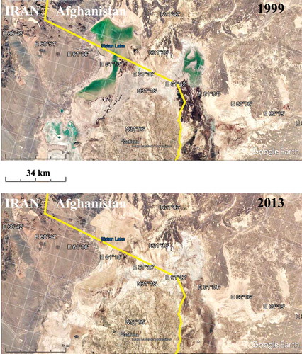
Hamum wetlands, Seistan basin of the Helmand rivers on the eastern border of Iran (bordered by Afghanistan) were selected for testing the methodology, see Figure 1. They are described in detail in the works (Kharazmi et al., 2017, 2016). Monthly multispectral images of Landsat 5 and Landsat 8 were used for the time interval 2015–2016.

Figure 1. Google-Earth images of Hamum wetlands dated 1999 and 2013 years, that illustrate the variability of wetting.

We used topological invariants, Betty numbers, represented by the persistence diagrams (PDs) as descriptors of digital images (Makarenko et al., 2015). Figure 2 shows an example of the PD.

Figure 2. (a) A fragment of the swamp landscape (02/25/2015). (b) the PDs for this image. Blue colour corresponds to the connected components, red color to the holes. The number of points in each clouds is shown in the legend. (c) A persistent image for the PD(${\beta }_1$).

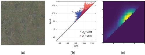
For each PD a persistent image was obtained (Adams et al., 2017), which serves as a pdf rating (see Figure 2, c). The semi-density is obtained by extracting the square root of the resulting matrices, converted into a row vector. The metric was the Hilbert scalar product of semi-densities in the tangent bundle to the unit sphere.

Figure 3. Comparative dynamics of natural complexes, represented by the Riemannian metric relative to the Karcher mean for the connected components, dim0_rdist, and holes, dim_1rdist: (a) the variability of the relative Riemannian distance for 2015; (b) the variability of the relative Riemannian distance for 2016. On the x-axis, the months and dates of the image are shown in a format (month_date).

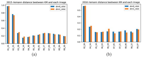
Our results are summarized in Figure 3. It shows the seasonal dynamics of the above areas, expressed in monthly deviations of the Riemannian semi-density from the Karcher average. The differences in texture variability at the 2-year interval are well noticeable. So, the pronounced autumn variability of the textural morphology of 2015 is practically absent in 2016.

4. Conclusion

The article describes the use of methods of discrete differential geometry for diagnosing patterns of digital images of landscapes, expressed by topological descriptors. This technique is designed to analyze the dynamics of the underlying surface in the case of its high temporal variation and the absence of clear spectral boundaries between the classes.

Topological Data Analysis, TDA, has three obvious advantages. The first of these is the simplicity of the signs—they are the ordered values of the photometric measure in pixels. The second is the multiresolution property: all scales are analyzed in the feature space. Finally, the third advantage is the invariant nature of the descriptors obtained: the Betti numbers do not need any a priori model, which is necessary for the traditional methods of spectral classification.

As an example, the article considers the satellite monitoring of wetlands in arid territories. The comparative morphological dynamics was analyzed on a 2-year interval based on topological descriptors. For the time sequence of descriptors obtained in the form of PD, estimates of pdf and their semi-densities were obtained, i.e. $\sqrt{pdf}$. The resulting unit Riemannian sphere, as the support of semidifinities, was equipped with a tangent bundle with a Hilbert scalar product. This design allows to measure the Riemannian distance between points, (i.e., pdf) in the angular measure; estimate the distance between them and calculate the average by Karcher on the sphere. We have shown that a change in the Riemannian distance relative to the average makes it possible to track the seasonal dynamics of landscapes. Note that the spectral classification methods do not allow obtaining an integral descriptor suitable for these purposes. We hope that the proposed method will allow analyzing satellite images, with an estimate of the measure of proximity between them. The latter circumstance makes it possible to use it in the tasks of identifying climate signals in long-term changes in the morphology of landscapes.

Acknowledgements

We gratefully acknowledge the financial support of the Ministry of Education and Sciences, Republic of Kazakhstan (Grant AP05134227).

Additional information

Funding

The authors received no direct funding for this research.

Notes on contributors

Nikolai Makarenko

Nikolai Makarenko, Dr of technical science and Dr of Physical and Mathematical Sciences, Principal Researcher of Institute of Information and Computational Technologies, Almaty, Kazakhstan; Head of the Department of Mathematical Modeling of the Central Astronomical Observatory of the Russian Academy of Sciences, St. Petersburg, Russia. A member of the Board of the executive committee of Russian Neural Networks Society. Research interests: computer modeling of nonlinear systems, computational topology, fractal geometry, deterministic chaos, mathematical morphology, Artificial Neural Networks, analysis of remote sensing data. He has over 100 publications in various sources.

References

- Adams, H., Emerson, T., Kirby, M., Neville, R., Peterson, C., Shipman, P., & Ziegelmeier, L. (2017). Persistence images: A stable vector representation of persistent homology. The Journal of Machine Learning Research, 18(1), 218–9. https://dl.acm.org/doi/abs/10.5555/3122009.3122017.
- Amari, S. I. (2009). Divergence function, information monotonicity, and information geometry. In Workshop on information theoretic methods in science and engineering (WITMSE). Citeseer. https://pdfs.semanticscholar.org/38e3/62758eb79eebef0de7386f350a7705ac5280.pdf
- Amari, S. I., & Nagaoka, H. (2007). Methods of information geometry (Vol. 191). American Mathematical Soc.
- Bubenik, P. (2015). Statistical topological data analysis using persistence landscapes. The Journal of Machine Learning Research, 16(1), 77–102. https://dl.acm.org/doi/10.5555/2789272.2789275
- Carlsson, G. (2009). Topology and data. Bulletin of the American Mathematical Society, 46(2), 255–308. https://doi.org/10.1090/S0273-0979-09-01249-X
- Edelsbrunner, H., & Harer, J. (2009). Computational topology. An introduction. American Mathematical Society.
- Edelsbrunner, H., & Morozov, D. (2012). Persistent homology: Theory and practice (No. LBNL- 6037E). Lawrence Berkeley National Lab. (LBNL).
- Edelsbrunner, H., Virk, Z., & Wagner, H. (2019). Topological data analysis in information space. arXiv preprint arXiv:1903.08510. https://www.researchgate.net/publication/331916154_Topological_Data_Analysis_in_Information_Space
- Ghrist, R. (2008). Barcodes: The persistent topology of data. Bulletin of the American Mathematical Society, 45(1), 61–75. https://doi.org/10.1090/S0273-0979-07-01191-3
- Ghrist, R. (2018). Homological algebra and data. Mathematical Data, 25, 273. https://www.math.upenn.edu/~ghrist/preprints/HAD.pdf
- Ghrist, R. W. (2014). Elementary applied topology (Vol. 1). Createspace.
- Grenander, U. (2012). Regular structures: Lectures in pattern theory (Vol. 3). Springer Science & Business Media.
- Karcher, H. (1977). Riemannian center of mass and mollifier smoothing. Communications on Pure and Applied Mathematics, 30(5), 509–541. https://doi.org/10.1002/cpa.3160300502
- Kerber, M., Morozov, D., & Nigmetov, A. (2017). Geometry helps to compare persistence diagrams. Journal of Experimental Algorithmics (JEA), 22, 1–20. https://doi.org/10.1145/3064175
- Kharazmi, R., Panidi, E. A., & Chaban, L. N. (2017). Assessment of the arid ecosystems dynamics using results of automated processing of the multispectral satellite imagery time series. Sovremennye Problemy Distantsionnogo Zondirovaniya Zemli Iz Kosmosa, 14(3), 196–205. https://doi.org/10.21046/2070-7401-2017-14-3-196-205. (in Russian).
- Kharazmi, R., Panidi, E. A., & Karkon, V. M. (2016). Assessment of dry land ecosystem dynamics based on time series of satellite images. Sovremennye Problemy Distantsionnogo Zondirovaniya Zemli Iz Kosmosa, 13(5), 214–223. https://doi.org/10.21046/2070-7401-2016-13-5-214-223. (in Russian).
- Makarenko, N. G., Karimova, L. M., & Kruglun, О. А. (2014). Scaling properties of digital images of Earth landscape. Sovremennye Problemy Distantsionnogo Zondirovaniya Zemli Iz Kosmosa., 11(2), 26–37. (in Russian). http://jr.rse.cosmos.ru/article.aspx?id=129
- Makarenko, N. G., Urtiev, F. А., Knyazeva, I. S., Malkova, D. B., Park, I. T., & Karimova, L. M. (2015). Texture recognition in digital images by computational topology methods. Sovremennye Problemy Distantsionnogo Zondirovaniya Zemli Iz Kosmosa, 12(1), 131–144. (in Russian) http://jr.rse.cosmos.ru/article.aspx?id=1371
- Robins, V., Abernethy, J., Rooney, N., & Bradley, E. (2004). Topology and intelligent data analysis. Intelligent Data Analysis, 8(5), 505–515. https://doi.org/10.3233/IDA-2004-8507
- Robins, V., & Turner, K. (2016). Principal component analysis of persistent homology rank functions with case studies of spatial point patterns, sphere packing, and colloids. Physica D. Nonlinear Phenomena, 334, 99–117. https://doi.org/10.1016/j.physd.2016.03.007
- Srivastava, A., & Klassen, E. P. (2016). Functional and shape data analysis. Springer.