Stochastic facility location problem in a competitive situation: A game theory model for emergency financial services

Abstract

Facility location problems under conditions of uncertainty involve various situations, such as industrial plants, warehouses, distribution centers, and emergency services (ambulances, police cars). Because of this relevant matter, researchers have developed many mathematical optimization models that aim to establish a balance between costs and the quality of the services provided over recent decades. By and large, these proposals consider stochastic characteristics associated with demand uncertainty and the facilities’ availability. Since there is a lack of studies examining emergency financial services, we think of managing this kind of service in a competitive situation combining Game Theory and computer simulation. In addition to the usual stochastic conditions, this study introduces the use of a Nash equilibrium model that also incorporates uncertainties related to the actions of competitors applied to a dispute between two insurers as to where to locate their home insurance assistance bases. The focal point concept combined the results of a non-zero-sum game with those of the stochastic location model to define an unconventional strategy for the analyzed situation. The developed mathematical model provided more realistic location strategies compared to those obtained using traditional location models.

Keywords:

• computer simulation
• facility location
• game theory
• mathematical model

PUBLIC INTEREST STATEMENT

Facility location is a common and costly decision that many public and private-sector companies face with social, economic, and environmental impacts. Due to its relevance, the facility location problem has encouraged engineers to come up with sophisticated models to support organizations’ decisions. Most of the copious literature has focused on the zero-sum game; in other words, one player’s gains emerge from the other’s losses. This study expands the location models’ applications to include a new and unexplored emergency financial services category from an engineering perspective based on an unusual non-zero-sum game. This work proposes a novel framework of comparison between players by a standardized asymmetry payoff matrix based upon geo-information data about the participants. We tested the model in a location dispute between two insurers in the northern region of São Paulo city in Brazil with promising results.

1. Introduction

Location is the identification of objects in a physical space. These objects can be facilities to achieve specific goals. According to ReVelle and Eiselt (2005), location analysis refers to the modeling, formulation, and solution of a class of problems described as sitting facilities in a given space. Slack et al. (2002) stress that location decisions are relevant because they are almost irreversible. Even when it is still possible to reverse the decision, it may be costly, time-consuming, and inconvenient for customers.

A facility location decision involves substantial financial and operational resources, significant setup times, and is difficult to reverse. Failures in this kind of analysis can affect the survival of companies that are in a competitive business. For this reason, researchers have developed many mathematical models in recent decades to find optimal locations for facilities (in industry, agriculture, service industries). The development of this approach has kept pace with the variety and complexity of many real problems. New proposals have been made over time to correct the conceptual weaknesses of previous models. The latest suggestions improved on previous ones but did not exclude them, creating an overlap and the coexistence of all the available alternatives. Snyder (2006) divided facility location models into a) deterministic, b) stochastic, or c) robust optimization.

Facility location problems present many challenges. It demands a lot of data about the participants’ geo-location, the provided service’s demand behavior, infrastructure availability, costs, and legislation restrictions. Usually, this kind of application requires considerable computer resources.

Emergency services comprise various situations that require the urgent intervention of the authorities or the service provider. We can find the term emergency financial service in the literature as a synonym of financial assistance provided by public or private sectors to support general needs (Palmer et al., 2019). In terms of financial services, studies exist for operations and the location of traditional banking facilities, such as bank branches (Abensur, 2011; Ajiboye, 2020; Basar et al., 2015; Gorener et al., 2013).

The relevance and diversification of the financial market offer an innovative niche for facility location applications. Nonetheless, no studies explore the facility location of emergency services in the financial sector carried out far away from the traditional branch network.

Home insurance service is an example of this category. It generally comprises two types: a) cover for unpredictable damage caused by fire, explosion, storms, and b) home assistance, which deals with minor problems, such as broken locks, leaking pipes, electrical problems, heating system problems, and so on. In general, other covers such as automobile insurance offer home assistance as a complimentary service. When required, this kind of service is requested remotely by contacting the insurer’s call center. The call center then classifies the request and activates the assistance team. Using authorized vehicles, the assistance team goes to customers’ houses from its service base to provide the service requested in the minimum amount of time possible. In general, the call center and the base service facility are in different places.

This study focuses on a particular part of the emergency financial process by examining possible optimization alternatives to facilities’ location in a competitive context. We proposed a Nash equilibrium model that can support emergency financial service facilities’ location through a classical duopoly game. We tested the model in a location dispute between two competing insurers (players) seeking to locate their emergency home insurance facilities in the northern region of the city of São Paulo in Brazil. The Game Theory (GT) model achieved more realistic results than the deterministic and stochastic location models. As provided by Google Maps, the land route distances between the proposed service bases and customers were incorporated into the analysis, which increased the model’s reliability.

The strengths and contributions of this work are:

• It expands the applications of location models to include a new and unexplored category of financial services carried out far away from the traditional banking branch;

• Unlike classic game theory approaches, composed of socio-economic features, such as price and customer behavior, the presented model uses the geo-location characteristics of the participants from an engineering perspective;

• It shows that traditional facility location models, which are characterized by having an individualistic perspective and are inappropriate in competitive situations, such as the analyzed, studied case;

• It presents a model that combines concepts of traditional location models with ideas of competitive location, based on a non-zero-sum emergency financial service game played by two competitors (players);

• The developed model offered a broader range of feasible alternatives, including strategies obtained using traditional location models;

• The study proposes a novel framework of comparison between players (and the models) by a standardized asymmetry payoff matrix based upon geo-information data about the participants.

• This study is structured as follows. In Section 2, we present a review of the literature on facility location models. In Section 3, we describe the characteristics of the analyzed problem, the type of game that was analyzed, and the respective mathematical model. In Section 4, we describe the case that was studied and the results found. In Section 5, we provide conclusions and future works.

2. Literature review

2.1. Deterministic location models

Deterministic models consider that the required parameters are known. Among these parameters are: costs, service demand, service level agreements, the distance between customers and the facilities, and the area covered. Generally, deterministic models divide the objectives into two types: i) the minimum number of facilities needed to cover demand, considering a defined distance or time limit; and ii) locating a known number of facilities to maximize the number of requests covered within a specified time limit.

The Type (i) model, also known as a set covering problem, was proposed initially by Toregas et al. (1971) and is used to find the minimum number of vehicles needed to cover all demands in a predefined time limit. Church and ReVelle (1974) proposed the Type (ii) model called a maximal covering location problem. There are other studies and applications, such as those by Amin and Zhang (2013), Anagnostopoulos et al. (2004), Daskin and Stern (1981), Li et al. (2011), Manopiniwes and Irohara (2017), Pérez et al. (2015), Prabowo et al. (2017), ReVelle et al. (1977), Verma and Gaukler (2015), Yadav et al. (2017), and Zhang et al. (2017).

2.2. Stochastic location models

Stochastic models improved the perspective of deterministic models by considering that facilities may not be available all the time. Deterministic models also assume that the probability of the facilities being busy or not (idleness) is the same for all of them. Thanks to stochastic models, it was possible to incorporate demand uncertainty, the uncertainty of the facilities being available (not busy), and other volatilities using many probability distributions. The main difference between stochastic models lies in their treatment of system reliability. Defined reliability problems aim to locate facilities with a known α probability of availability. Maximum availability location problems aim to install facilities that provide the most significant availability probability (Ahmadi-Javid & Nasrin, 2020; Balcik & Beamon, 2008; Daskin, 1983; Drezner et al., 2015; ReVelle & Hogan, 1989; An et al., 2014).

The system’s idleness rate, travel time, and service times are factors that combine queuing theory with stochastic location problems. This kind of model’s relevant contribution is how it estimates facilities’ availability within a time or distance standard (Jung et al., 2014; Larson, 1975; Liu et al., 2020; Marianov & ReVelle, 1996; Tavakkoli-Moghaddam et al., 2016).

Equations (1)(1) $\begin{array}{rl}& min{Z}_{\hspace{0.17em}}=\sum _{j\in J}^{\hspace{0.17em}}{X}_{J\hspace{0.17em}}\hspace{0.17em}\\ & s.a.\end{array}$(1) to (3) and (4) to (6) give examples of a deterministic location model (Daskin, 2008) and a stochastic model (ReVelle & Hogan, 1989), respectively. Equation (1)(1) $\begin{array}{rl}& min{Z}_{\hspace{0.17em}}=\sum _{j\in J}^{\hspace{0.17em}}{X}_{J\hspace{0.17em}}\hspace{0.17em}\\ & s.a.\end{array}$(1) minimizes the number of facilities j needed to cover all the demand. Equation (2)(2) $\sum _{j\in N_i}^{\hspace{0.17em}}{X}_J\ge 1\hspace{0.17em}\mathrm{\forall }i\in I\hspace{0.17em}$(2) requires that each node be covered: Let J be a set of potential locations, and I be a set of demand nodes; the distances d_ij from node i ∈ I to the possible location j ∈ J is known. Equation (3)(3) $X_J\in \{0,1\}\hspace{0.17em}\mathrm{\forall }j\in J$(3) requires integer and binary variables. In the stochastic formulation, (5) represents the reliability of at least one facility is available to users at a defined probability α. Let q be the probability of all N_i facilities being busy and b be the smallest integer number that satisfies the ratio presented.

(1) $\begin{array}{rl}& min{Z}_{\hspace{0.17em}}=\sum _{j\in J}^{\hspace{0.17em}}{X}_{J\hspace{0.17em}}\hspace{0.17em}\\ & s.a.\end{array}$(1)

(2) $\sum _{j\in N_i}^{\hspace{0.17em}}{X}_J\ge 1\hspace{0.17em}\mathrm{\forall }i\in I\hspace{0.17em}$(2)

(3) $X_J\in \{0,1\}\hspace{0.17em}\mathrm{\forall }j\in J$(3)

(4) $\begin{array}{rl}& min{Z}_{\hspace{0.17em}}=\sum _{j\in J}^{\hspace{0.17em}}{X}_{J\hspace{0.17em}}\hspace{0.17em}\\ & s.a.\end{array}$(4)

(5) $\sum _{j\in N_i}^{\hspace{0.17em}}{X}_J\ge b_i\hspace{0.17em}\mathrm{\forall }i\in I\hspace{0.17em}$(5)

(6) $X_j\ge 0\mathrm{i}\mathrm{n}\mathrm{t}\mathrm{e}\mathrm{g}\mathrm{e}\mathrm{r}$(6)

where:

$b=\frac{log(1-\alpha )}{logq}$

2.3. Robust models

Robust models appear in situations where it is difficult to collect data, or there is a lack of data about the probability distribution of the analyzed parameters. According to Snyder (2006), the two most crucial robustness measures are minimax cost and minimax regret. This category of models features stochastic treatment applied to the analyzed parameters. The scenario approach is applied to discrete cases, while continuous ones use interval uncertainties (Kouvelis et al., 2000; Kouvelis & Yu, 2013; Listes & Dekker, 2005; Rabbani et al., 2020; Snyder & Daskin, 2006; Zhang & Jiang, 2014).

2.4. Location models based on game theory

The previous approaches display passive behavior in the competition. Managers suppose the facilities will be available as long as necessary. This attitude is highly unfavorable in competitive environments because competitors can occupy all the already identified locations or the best ones. Thus, a new hybrid category emerged called competitive location problems, which add to the uncertainty surrounding competitors’ actions (ReVelle & Eiselt, 2005). This category is also known as Hotelling’s location model because Hotelling (1929) developed an optimal facility location model and two competitors’ pricing along a straight-line segment. Nash equilibrium is the solution to this problem category, in which there are no reasons for competitors to change their positions.

New studies present other cases of competitive facility location that combine stochastic techniques and the game theory (Camacho-Vallejo et al., 2014; Fernández & Hendrix, 2013; Giménez-Gaydou et al., 2016; Herbon, 2017; Mayadunne et al., 2018; Moradi et al., 2016; Patne et al., 2018; Salazar et al., 2018; Seyhan et al., 2018; Song & Wen, 2015; Yin et al., 2016).

3. Problem detailing and the mathematical game model

Table 1 shows the symbols used in developing the mathematical formulation of the game.

Table 1. Symbol description

Symbol	Description
SLA	Service Level Agreement
r	The critical distance that makes SLA possible
M/M/m/k	Poisson distributed assistance request rate (M), generally distributed service times (M), m = 1 server, maximum service capacity equal to k customers
λ	Average call rate
µ	The average service time rate
S	Location strategy
i	Facility index
j	Customer index
I	Number of facilities
J	Number of customers
P0	Probability of the facility not being busy
ρ	Facility busy rate (λ/µ)
ξ	Poisson distribution to generate residentially assistance calls
c	Customer
dij	Distance between customer i and facility j
w	The random number generated by a uniform distribution
x	Facility location for player A
y	Facility location for player B

The case studied analyzes the dispute between two similar Brazilian insurers who simultaneously decide on their home insurance assistance bases in the north region of São Paulo city, chosen from five potential sites (A, B, C D, E). According to official figures, the city of São Paulo has 12 million inhabitants and is the largest city on the American continent. There are 7.2 million automobiles and 6 million motorcycles, while 14,000 buses run daily. In addition to the large population and vehicle density, the city of São Paulo has an irregular topography with valleys, rivers, hills, and mountains making urban mobility a daily challenge.

Brazilian insurers generally offer their customers a similar kind of home assistance insurance cover. Following the rules defined by the Brazilian insurance regulatory agency (SUSEP), the insurers have two hours (SLA) to complete the service. Despite the similarities, after-sales service is a significant differential for ensuring customer satisfaction. As a result, the facilities’ location is a decisive strategic variable that can reduce customer dissatisfaction and the resultant loss of their business in São Paulo city.

We adjusted the data concerning customer location, potential facility locations, and service demand from one of the players. There are 104 customers in this region, and dissatisfaction levels are high due to service complaints.

Call centers receive emergency assistance calls made by phone or via an app and select the nearest facility location. Service employees leave these locations to attend to customers’ demands. The decision and the game are related to the site of these facilities. Calls are random and occur independently between customers in the analyzed region. According to service features, we adopted the following assumptions:

a) just one employee at each facility (m = 1);

b) competitors cannot share the same facility;

c) each customer only makes one call per month;

d) a critical distance (r) of 3 km was defined as the maximum feasible distance from which to handle calls following the defined SLA;

e) a maximum of three service callouts is achieved per day;

f) unavailable facilities or out-of-SLA service results in different penalties for insurers;

g) random calls were generated every month to assess all customers;

h) facility costs were considered to be similar for the companies;

i) under the studied statistical data, we evaluated the following: λ = six calls per month (6% or 0.06 considering 104 customers) and μ = 22 services per Month/employee/facility.

There are three primary sources of uncertainty: customer call’s location, facility unavailability (busy), and the actions of competitors.

We assessed the probability Z of home assistance calls using a Poisson distribution, with k being the probability of a monthly call demand. We evaluated the non-busy probability (P₀) using the M/M/m/k queuing system like Marianov and ReVelle (1996), shown in Equation 7(7) $P_0=\hspace{0.17em}\left\{\begin{array}{c}\frac{1-\rho }{1-{\rho }^{K+1}},\rho \ne 1\\ \frac{1}{K+1},\rho =1\end{array}\right\}$(7) as follows.

Firstly, each competitor has six strategies: a) choosing no location; b) choosing 1; c) choosing 2; d) choosing 3; e) choosing 4, or f) choosing five sites. There is no cooperation between the competitors (companies), and both know the game’s strategies and payoffs.

Competitors can only rent different facilities, and they cannot share them. The competitors choose their locations and send their proposals to the owners. If there are two proposals for the same place, the renting process will take more time, and both companies would be without a home assistance base for at least the next month. Other combination choices result in different payoffs for the players.

Due to the possible location strategies, each player’s payoffs reduce service penalties by the SLA. Two or three places are the best strategy for both competitors because other alternatives are dominated by this one or present lower payoff. Not sharing locations imply logistic asymmetry in terms of the number of facilities per insurer and their customers’ distances. Every strategy will result in different penalties for each player as a non-zero-sum game. Therefore, the game is defined as a) non-zero-sum; b) simultaneous, and c) non-cooperative.

Figure 1 shows the candidate service bases’ location and the defined critical distance obtained using land routes in this region. Table 2 presents the complete list of distances between customers and potential facility locations.

Table 2. Matrix of distances between customers and candidate facilities (meters)

Customer	A	B	C	D	E	Customer	A	B	C	D	E
1	2,750	2,800	2,400	2,700	3,400	53	2,800	3,100	2,700	2,800	3,100
2	2,900	4,500	4,100	2,600	2,600	54	2,650	3,800	3,400	2,900	2,600
3	4,600	2,900	140	4,700	4,500	55	2,500	3,700	3,200	2,700	2,800
4	3,500	3,400	2,500	3,300	3,600	56	2,650	4,100	2,700	2,900	2,300
5	3,400	2,300	1,900	3,400	4,100	57	2,750	4,000	2,500	3,000	2,400
6	2,250	3,800	3,400	2,500	2,600	58	2,600	4,100	2,700	2,900	2,200
7	2,350	3,300	2,900	2,400	3,000	59	2,900	4,200	2,400	3,100	2,500
8	3,100	3,400	2,100	3,300	3,000	60	2,900	4,200	2,400	3,100	2,500
9	3,100	3,400	2,100	3,300	2,900	61	2,650	4,100	2,700	2,900	2,300
10	2,500	3,200	2,700	2,500	3,200	62	3,100	3,500	2,200	3,300	2,900
11	2,700	3,900	3,500	3,000	2,500	63	3,100	3,400	2,000	3,300	2,700
12	2,650	3,800	3,400	2,900	2,600	64	3,100	3,400	2,000	3,300	2,700
13	2,750	3,900	3,500	3,000	2,500	65	4,200	4,000	1,600	4,200	3,000
14	2,600	3,800	3,300	2,900	2,600	66	4,100	3,900	2,400	4,100	2,800
15	2,650	3,800	3,400	2,900	2,600	67	2,550	3,300	2,900	2,500	3,000
16	2,750	4,000	2,500	3,000	2,400	68	2,210	3,700	3,300	2,300	2,900
17	2,750	4,000	2,500	3,000	2,400	69	3,000	3,500	2,600	2,900	3,600
18	2,650	4,100	2,700	2,900	2,300	70	3,000	4,200	2,500	3,200	2,200
19	2,750	4,000	2,500	3,000	2,400	71	2,800	3,500	2,400	3,100	2,700
20	2,750	4,000	2,500	3,000	2,400	72	2,800	3,500	2,400	3,100	2,700
21	2,600	4,200	2,700	2,800	2,200	73	2,850	4,200	2,700	3,100	2,000
22	2,650	4,100	2,700	2,900	2,300	74	2,900	2,800	2,400	2,900	3,600
23	2,700	3,900	3,400	3,000	2,500	75	3,000	2,600	2,200	3,000	3,700
24	2,600	4,000	3,300	2,900	2,600	76	3,000	2,600	2,200	3,000	3,700
25	3,200	2,700	2,300	3,100	3,700	77	3,000	2,600	2,200	3,000	3,700
26	3,400	2,600	2,200	3,400	4,000	78	3,000	2,600	2,200	3,000	3,700
27	4,200	4,000	1,700	4,200	3,000	79	3,000	2,600	2,200	3,000	3,700
28	3,000	3,500	2,600	2,900	3,600	80	3,100	3,000	2,500	3,100	3,600
29	2,800	3,500	2,400	3,000	2,800	81	2,550	3,300	2,900	2,500	3,200
30	3,000	2,800	2,300	2,900	3,500	82	4,200	4,000	2,500	4,200	2,700
31	3,000	2,800	2,300	2,900	3,600	83	4,200	4,000	2,500	4,200	2,700
32	3,000	2,600	2,200	3,000	3,700	84	3,500	2,100	1,700	3,400	4,100
33	4,000	3,500	1,300	4,000	3,300	85	2,650	3,800	3,400	2,900	2,700
34	3,200	3,400	1,900	3,500	2,700	86	2,600	3,500	2,500	2,900	3,000
35	3,500	3,600	2,200	3,700	2,400	87	2,550	3,200	2,800	2,600	3,200
36	2,700	3,800	2,500	2,900	2,800	88	3,200	3,200	2,300	3,400	3,300
37	2,700	3,800	2,500	2,900	2,800	89	4,200	4,000	1,900	4,100	2,600
38	2,600	4,200	3,800	2,900	2,100	90	3,300	2,300	1,900	3,300	3,800
39	3,900	3,700	2,200	3,900	3,000	91	2,350	3,900	3,400	2,600	2,700
40	3,600	2,300	1,900	3,500	4,100	92	2,450	4,000	3,600	2,700	2,800
41	3,000	2,600	2,200	3,000	3,500	93	2,350	3,900	3,400	2,600	2,700
42	2,500	4,000	3,600	2,800	2,900	94	2,350	3,900	3,400	2,600	2,700
43	3,000	2,900	2,400	3,000	3,700	95	2,600	4,100	3,700	2,900	3,000
44	2,550	3,500	2,400	2,800	2,900	96	2,750	3,400	2,500	3,000	2,800
45	3,900	3,700	2,200	3,900	3,000	97	3,000	2,900	2,400	3,000	3,700
46	4,200	4,000	1,900	4,200	2,700	98	2,950	2,700	2,300	2,900	3,600
47	2,750	3,200	2,200	3,000	3,100	99	3,700	3,700	2,200	3,900	2,400
48	4,000	4,100	2,600	4,300	2,800	100	2,800	3,500	2,400	3,100	2,700
49	2,500	3,200	2,700	2,500	3,200	101	2,750	4,000	2,500	3,000	2,400
50	2,450	3,200	2,800	2,400	3,100	102	2,094	3,700	3,300	2,300	2,700
51	2,500	3,200	2,700	2,500	3,200	103	2,094	3,700	3,300	2,300	2,700
52	2,750	3,000	2,600	2,800	3,200	104	2,079	3,700	3,300	2,300	2,700

Source: Prepared by the authors

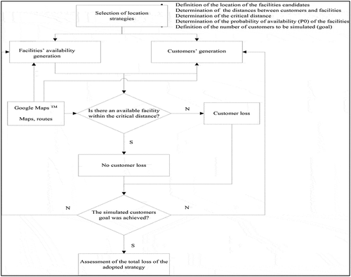
Figure 2 shows the simulation logic flow that evaluates each feasible location strategy’s players’ payoffs. The following parameters are first defined: a) potential facility locations (A, B, C, D, E); b) land route distances from customers (meters) provided by Google Maps; c) the critical distance (r), and d) the not busy probability P₀ and the number of customers to be evaluated. The Poisson distribution and uniform distribution randomly generate the customers’ calls and facility availability, respectively. The penalty depends on whether there is an available facility within the critical distance. We adopted weight 1 for facilities beyond the crucial range and value 2 for facilities unavailable for providing service. We repeated the simulation to assess all customers.

Figure 1. Candidate service bases and critical distances

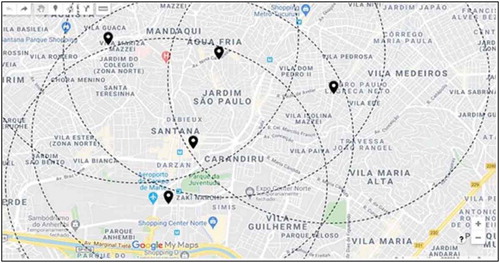
Figure 2. The logical flow of the simulation

Let G = (X, Y, M) represent the analyzed game in its normal form. X and Y are finite sets of possible location strategies, and M is the payoff (penalty) function of the space of combinations X × Y of pairs (x,y), x ∈ X, y ∈ Y. The following vectors define the possible pure strategies S_X,Y for each player:

S_X = {x₁, x₂, x₃, x₄, x₅} and S_Y = {y₁, y₂, y₃, y₄, y₅} with x_i, y_i ∈ {0,1}

On the other hand, M is a function of a) the chosen location strategies S_X,Y, b) the defined critical distance (r); c) the land route distances between customers and facilities (d_ij); d) the not busy probability (P₀) and e) customer assistance calls (ξ).

d_ij = |x_i—c_j| or d_ij = |y_i—c_j| with i ∈ {0,1,2, …., I} facilities and j ∈ {0,1,2, …., J} customers

(7) $P_0=\hspace{0.17em}\left\{\begin{array}{c}\frac{1-\rho }{1-{\rho }^{K+1}},\rho \ne 1\\ \frac{1}{K+1},\rho =1\end{array}\right\}$(7)

(8) $F(w)=P(W\le w)=\underset{0}{\overset{1}{\int }}f(w)dw=\left\{\begin{array}{c}0ifw<0\\ wif0\le w\le 1\\ 1\hspace{0.17em}ifw>1\end{array}\right\}$(8)

(9) $\xi (Z=k)=\hspace{0.17em}\frac{{\alpha }^k{e}^{-\alpha }}{k!}$(9)

The players’ matrix of penalties is defined as follows:

$M(x,y)=\hspace{0.17em}\left\{\begin{array}{c}2if\xi (Z)\ge 1andw>P_0\\ \\ 1if\xi (Z)\ge 1,w\le P_0,\left|xi-cj\right|>r\mathrm{a}\mathrm{n}\mathrm{d}\left|yi-cj\right|>r\\ \\ 0if\xi (Z)\ge 1,w\le P_0,\left|xi-cj\right|\le r\mathrm{a}\mathrm{n}\mathrm{d}\left|yi-cj\right|\le r\end{array}\right\}$

$x_i,y_i\in \left\{0,1\right\}and{x}_i+y_i\le 1$

Let the n x m matrices A and B be the payoff matrices to players I and II, respectively. Assuming that for each strategy A_ij of player I, the best response of player II is B(i^B, j^B), and for each strategy B_ij of player II the best response of player I is A(i^A, j^A). Player I maximizes over the rows of A, and player II maximizes over the columns of B. The Nash equilibrium defines the point (A⁰_{i j}, B⁰_{i j}) as a pair of strategies A(i^A, j^A) and B(i^B, j^B) where it fulfills the objectives simultaneously. More precisely, we have:

${A^0}_i=max\left(A_{ij}\right)\wedge {B^0}_{ij}=max\left(B_{ij}\right)\Rightarrow \left(i^A{,}_{\hspace{0.17em}}{j}^A\right)=\left(i^B{,}_{\hspace{0.17em}}{j}^B\right)=\left({{ }_i}^0{{ }_{,j}}^0\right)$

Some of the Nash equilibriums found (in bold) are presented in Table 3 as follows.

Table 3. Matrix of penalties

	01010	01001	00110	00101	00011
01010	-	-	-	(194;39)	-
01001	-	-	(143;39)	-	-
00110	-	(39;143)	-	-	-
00101	(39;194)	-	-	-	-
00011	-	-	-	-	-
01100	-	-	-	-	(183;101)
11000	-	-	(153;39)	(153;39)	(153;101)
10100	(35;194)	(35;143)	-	-	(35;101)
10010	-	(72;143)	-	(72;39)	-
10001	(98;194)	-	(98;39)	-	-
01110	-	-	-	-	-
01101	-	-	-	-	-
01011	-	-	-	-	-
00111	-	-	-	-	-
11100	-	-	-	-	(26;101)
11010	-	-	-	(122;39)	-
11001	-	-	(42;39)	-	-
10101	(10;194)	-	-	-	-
10011	-	-	-	-	-
10110	-	(17;143)	-	-	-

4. Results

We obtained the results using MATLAB of MathWorks®. The following theorem defines mixed strategies (Blackwell & Girshick, 1979):

Theorem 1: Every finite game has a value, and each player has at least one good mixed strategy.

Marianov and ReVelle (1996) noted that the not busy probability of facilities P₀ was evaluated by the queuing system M/M/m/K, as shown in Table 4. We used this probability subsequently for simulating the stochastic location model. We converted all values to calls per month. Table 5 presents the optimal mixed strategies obtained, while Table 6 provides a comparison of the results found by the analyzed optimization models.

Table 4. M/M/m/K queueing system indexes

System	λ	µ	ρ	P0
M/M/1/3	6 customers/month	22 customers/month	27.27%	91%

Source: Prepared by the authors

Table 5. Mixed strategies evaluation

	Player	A
Player B	2 locations (q)	3 locations (1-q)	q-mix
2 locations (p)
Player A strategy	(00110)	(01011)
penalty	39	46	39q +46 (1-q)
Player B strategy	(10001)	(10100)
penalty	98	35
3 locations (1-p)
Player A strategy	(10100)	(11001)
penalty	35	1194	35q + 1194(1-q)
Player B strategy	(01011)	(11001)
penalty	46	1194
p-mix	98p + 46(1-p)	35p + 1194(1-p)

Source: Prepared by the authors

Table 6. Optimization models comparison

	Game Theory				Deter. Model	Stoch. Model (α=0.90) (P0=0.91)	Stoch. Model (α=0.95) (P0=0.91)
Player A	(00110)	(10100)	(11001)	(01011)	(00101)	(00101)	(00110)
Player B	(11001)	(01011)	(00110)	(10100)	-	-	-
Total Penalty	81	81	81	81	111	111	81
Difference %	7.7	31.4	7.7	25.0	84.6	84.6	7.7
Mixed strategy player A	(00110) (11001)	q=0.99	-	-	-	-	-
Expected penalty player A	39	-	-	-	-	-	-
Mixed strategy player B	(10001) (01110)	p=0.94	-	-	-	-	-
Expected penalty player B	98	-	-	-	-	-	-
Total Penalty	137	-	-	-	-	-	-
Focal Point Strategy A	(11001)	-	-	-	-	-	-
Focal Point Strategy B	(00110)	-	-	-	-	-	-
Total Penalty	81	-	-	-	-	-	-

Source: Prepared by the authors

We analyzed the results from the perspective of Player A. We found twenty Nash equilibriums in pure strategies. For the evaluations and comparisons shown in Tables 5 and 6, we selected a subset of pairs that gave the lowest absolute sum of penalties for two and three locations under the restriction of not sharing facilities.

According to the definition of the problem, the game is simultaneous and non-cooperative. Therefore, players must consider the probability of their competitor choosing a strategy. Players A and B can select two or three locations. We assume p and (1-p) to be, respectively, the probability of Player B choosing two or three places. We also considered q as the probability that Player A would choose two locations and (1-q) the likelihood of it selecting three sites. In equilibrium, each player must choose a p and q mix that represents the best response to the p and q combination of the respective competitor. Thus, the best comeback of Player A must show the best q for each value of Player B’s p, and vice versa. As explained in Section 3, the choice of three locations would be unfavorable in both companies and, therefore, we penalized with the highest value obtained in the simulations (1,194 points). We found the mixed strategy by solving the p-mix and q-mix equations shown in Table 5 as follows.

Figure 3 presents the graphic representation of the Nash equilibrium in mixed strategies. If q < 0.94, the optimal response for B is p = 1; in other words, the best choice is two locations. If q > 0.94, the optimum comeback for B is p = 0; in other words, the optimal choice is three locations; finally, if q = 0.94, two or three sites are equal best choices for B.

Figure 3. Nash equilibrium in mixed strategies

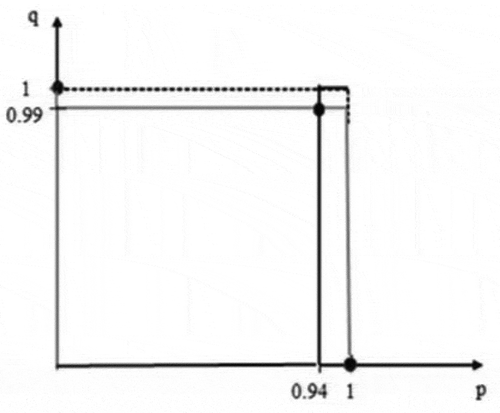
According to Dixit et al. (2015), we should use mixed-strategies in non-zero-sum games with considerable caution. There is no general reason why one player’s pursuit of their interests should work against the other player’s interests in such games. Therefore, one player would not generally want to conceal their intentions from the other player, and there is no general argument in favor of keeping the other player guessing. In the case analyzed, we can understand the mixed strategies as both players choosing two locations with a high probability in their optimal mixtures (p = 0.94 and q = 0.99), which could lead to severe losses if both choose the same locations.

As presented in Table 6, a comparison between the models was standardized by the game theory model’s penalty function. The total value of the strategic pair is the sum of the penalties for each player. We measured the penalty asymmetry between players by the relative distance between the players’ penalty value in the respective strategic pair. The game theory model provides more location alternatives by assuming that one competitor can obtain more locations. The game theory model also gave more realistic results than deterministic and stochastic models in terms of penalties.

Traditional location models do not consider competitor reactions. The deterministic model considers only the distance between the customer and the facilities. There is no stochastic appreciation of the availability of facilities or call demand. As expected, the deterministic model gave fewer locations (2), but the total penalty was higher than with the game theory model. By the same criterion, the stochastic models with α = 0.90 and α = 0.95 obtained results that were respectively inferior to and equal to those of the game theory model, but this also disregards the stochastic demand condition of the number of calls per customer.

The focal point concept emerges as a refinement in cases where there are multiple Nash’s equilibriums. Thus, it helps find a convergence between players’ strategies to avoid bad choices. The stochastic model shows that two locations are within the critical distance to all customers. Since rational players play the game, choosing two sites is a realistic option. Thus, choosing the other three locations should be a feasible strategy since it avoids proposals overlap.

The focal point strategy, however, does not guarantee convergence. Practical actions are necessary to coordinate the players’ expectations. In this case, a rapid negotiation of the facilities associated with disclosure of the new service locations on the company’s institutional website, for example, would help clarify the alternatives to be followed by the other player.

Table 7 and Figure 4 present the sensitivity analysis of the model. As explained in Section 3, we did not consider any gain related to the critical distance we adopted (3,000 m). We assumed changes in call demand and the not busy of the facility. Following current conditions, in other words, one employee at each location and an average call rate equal to 6% per month (P₀ = 0.91 e ξ = 0.06), the proposed strategy can ensure twice the number of variations in call demand. Still, it is highly sensitive to reductions in availability. We can obtain reductions in waiting time by increasing the number of employees at each location.

Figure 4. The penalty due to call demand and facility availability

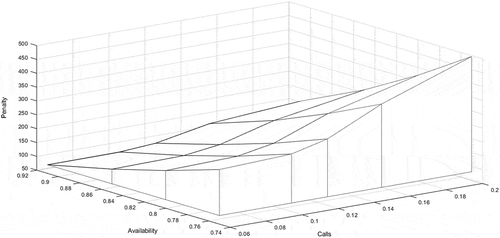
Table 7. Sensitivity Analysis for player A (11,001) and player B (00110)

			ξ (Z = k)
P0	0.06	0.10	0.12	0.15	0.20
0.91	81	82	91	128	152
0.85	134	138	155	208	262
0.80	186	193	217	290	372
0.75	247	258	290	382	497

Source: Prepared by the authors

5. Conclusion and future works

This work proposed a decision location model based upon the game theory, which was tested by way of a non-zero-sum game between two insurers competing for home assistance facility locations in the north region of São Paulo city in Brazil. This work has contributed to the literature by developing an approach that combines the logistic characteristics of location, demand, availability, geo-location technologies with Nash’s equilibrium concepts to define sustainable strategies for the analyzed companies.

Instead of the individualistic perspective of classical location models, the proposed model introduced competitors’ actions, allowing for a more realistic assessment of facility location possibilities by providing a broader range of feasible alternatives. Moreover, we incorporated the game’s stochastic conditions under each customer’s location characteristics, and facility analyzed.

The best results show asymmetric numbers of locations between competitors; in other words, Player A could choose two or three sites, while Player B could choose three or two. Besides, and most importantly, the model identifies where each player should locate each facility to avoid losses. The results are unconventional because, according to conventional wisdom, each player would choose two facilities.

Besides the Nash equilibrium, we developed other topics, such as mixed strategies and focal points. In particular, the focal point concept combined the results of game theory with those of the stochastic location model to define a strategy for Player A by assigning three complementary locations. This strategy differs from the usual, individualistic practice that would minimize costs by selecting the two sites closest to all customers, but with a high chance of losses for both.

Future work should focus on improving the SLA defined by the Brazilian regulatory agency. The assumed SLA is, at the same time, an applications’ characteristic and weakness. As future directions, we see that further investigation into methods to support insurance regulatory agency could yield positive results.

Additional information

Funding

The authors received no direct funding for this research.

Notes on contributors

Eder Oliveira Abensur

Dr. Eder Oliveira Abensur is currently working as a Professor of Operations Research and Economic Engineering at the Federal University of ABC (UFABC) in Santo André, Brazil. His current research interests include equipment replacement policy models, financial engineering, machine learning, and operations research. Alexandre da Silva Paes, Erick Reyann Kasai Yamada, Vito Ruggieri, and Walquiria Alves de Aquino are management engineers by UFABC.

References

- Abensur, E. O. (2011). Banking operations using queuing theory and genetic algorithms. Produto & Produção, 12(2), 69–18. https://doi.org/10.22456/1983-8026.17548
- Ahmadi-Javid, A., & Nasrin, R. (2020). A stochastic location model for designing primary healthcare networks integrated with workforce cross-training. Operations Research for Health Care, 24, 1–9. https://doi.org/10.1016/j.orhc.2019.100226
- Ajiboye, M. R. (2020). A simulation model for customer flow analysis ina commercial bank in Nigeria. European Journal of Technique, 10(1), 64–74. https://doi.org/10.36222/ejt.683040
- Amin, S. H., & Zhang, G. (2013). A multi-objective facility location model for closed-loop supply chain network under uncertain demand and return. Applied Mathematical Modelling, 37(6), 4165–4176. https://doi.org/10.1016/j.apm.2012.09.039
- Anagnostopoulos, A., Bent, R., Upfal, E., & Hentenryck, P. V. (2004). A simple and deterministic competitive algorithm for online facility location. Information and Computation, 194(2), 175–202. https://doi.org/10.1016/j.ic.2004.06.002
- Balcik, B., & Beamon, M. (2008). Facility location in humanitarian relief. International Journal of Logistics Research and Applications, 11(2), 101–121. https://doi.org/10.1080/13675560701561789
- Basar, A., Kabak, O., Topçu, Y. I., & Bozkaya, B. (2015). Location analysis in banking: A new methodology and application for a turkish bank in applications of location analysis. Springer.
- Blackwell, D., & Girshick, M. A. (1979). Theory of games and statistical decisions. Dover Publications.
- Camacho-Vallejo, J. F., Cordero-Franco, A. E., & Gonzalez-Ramirez, R. G. (2014). Solving the bilevel facility location problem under preferences by a stackelberg-evolutionary algorithm. Mathematical Problems in Engineering, 1–14. https://doi.org/10.1155/2014/430243
- Church, R., & ReVelle, C. (1974). The maximal covering location problem. Papers of the Regional Science Association, 32(1), 101–118. https://doi.org/10.1007/BF01942293
- Daskin, M. (1983). A maximum expected covering location model: Formulation, properties, and heuristic solution. Transportation Science, 17(1), 48–70. https://doi.org/10.1287/trsc.17.1.48
- Daskin, M. (2008). What you should know about location modelling. Naval Research Logistics, 55(4), 283–294. https://doi.org/10.1002/nav.20284
- Daskin, M., & Stern, E. H. (1981). A hierarchical objective set covering model for emergency medical service vehicle deployment. Transportation Science, 15(2), 137–152. https://doi.org/10.1287/trsc.15.2.137
- Dixit, A., Skeath, S., & Reiley, D. (2015). Games of strategy. W.W. Norton & Company.
- Drezner, Z., Brimberg, J., Mladenovic, N., & Salhi, S. (2015). New heuristic algorithms for solving the planar p-median problem. Computers & Operations Research, 62, 296–304. https://doi.org/10.1016/j.cor.2014.05.010
- Fernández, J., & Hendrix, E. M. T. (2013). Recent insights in huff-like competitive facility location and design. European. Journal of Operational Research, 227(3), 581–584. https://doi.org/10.1016/j.ejor.2012.12.032
- Giménez-Gaydou, Ribeiro, D. A. A. S. N., Gutiérrez, J., & Antunes, A. P. (2016). Optimal location of battery electric vehicle charging stations in urban areas: A new approach. International Journal of Sustainable Transportation, 10(5), 393–405. https://doi.org/10.1080/15568318.2014.961620
- Gorener, A., Hasan, D., & Hacioglu, U. (2013). Application of multi-objective optimization on the basis of ratio analysis (MOORA) method for bank branch location selection. International Journal of Finance & Banking Studies, 2(2), 41–52. https://doi.org/10.20525/ijfbs.v2i2.145.
- Herbon, A. (2017). Non-cooperative game of a duopoly under asymmetric information on consumer location. International Journal of Production Research, 55(18), 5185–5201. https://doi.org/10.1080/00207543.2016.1278482
- Hotelling, H. (1929). Stability in Competition. The Economic Journal, 39(153), 41–57. https://doi.org/10.2307/2224214
- Jung, J., Chow, J. Y. J., Jayakrishnan, R., & Park, J. Y. (2014). Stochastic dynamic itinerary interception refueling location problem with queue delay for electric taxi charging stations. Transportation Research Part C, 40, 123–142. https://doi.org/10.1016/j.trc.2014.01.008
- Kouvelis, P., Daniels, R. L., & Vairaktarakis, G. (2000). Robust scheduling of a two-machine flow shop with uncertain processing times. IIE Transactions, 32(5), 421–432. https://doi.org/10.1080/07408170008963918
- Kouvelis, P., & Yu, G. (2013). Robust discrete optimization and its applications. Springer.
- Larson, R. C. (1975). Approximating the performance of urban emergency services systems. Operations Research, 23(5), 845–868. https://doi.org/10.1287/opre.23.5.845
- Li, X., Zhao, Z., Zu, X., & Wyatt, T. (2011). Covering models and optimization techniques for emergency response facility location and planning: A review. Mathematical Methods of Operations Research, 74(3), 281–310. https://doi.org/10.1007/s00186-011-0363-4
- Listes, O., & Dekker, R. (2005). A stochastic approach to a case study for product recovery network design. European Journal of Operational Research, 160(1), 268–287. https://doi.org/10.1016/j.ejor.2001.12.001
- Liu, Y., Dehghani, E., Jabalameli, M. S., Diabati, A., & Lu, -C.-C. (2020). A coordinated location-inventory problem with supply disruptions: A two-phase queuing theory–optimization model approach. Computers & Industrial Engineering, 142, 1–15. https://doi.org/10.1016/j.cie.2020.106326
- Manopiniwes, W., & Irohara, T. (2017). Stochastic optimisation model for integrated decisions on relief supply Chains: Preparedness for disaster response. International Journal of Production Research, 55(4), 979–996. https://doi.org/10.1080/00207543.2016.1211340
- Marianov, V., & ReVelle, C. (1996). The queueing maximal availability location problem: A model for the siting of emergency vehicles. European Journal of Operational Research, 93(1), 110–120. https://doi.org/10.1016/0377-2217(95)00182-4
- Mayadunne, S., Johar, M., & Saydam, C. (2018). Competitive store closing during an economic downturn. International Journal of Production Economics, 199,162-178. https://doi.org/10.1016/j.ijpe.2018.02.016
- Moradi, M. H., Abedini, M., & Hosseinian, S. M. (2016). A combination of evolutionary algorithms and game theory for optimal location and operation of DG from DG owner standpoints. IEEE Transactions on Smart Grid, 7(2), 608–616. http://doi.org/10.1109/TSG.2015.2422995
- Palmer, C., Phillips, D. C., & Sullivan, J. X. (2019). Does emergency financial assistance reduce crime? Journal of Public Economics, 169(17), 34–51. https://doi.org/10.1016/j.jpubeco.2018.10.012
- Patne, K., Shukla, N., Kiridera, S., & Tiwari, M. K. (2018). Solving closed-loop supply chain problems using game theoretic particle swarm optimisation. International Journal of Production Research, 56(17), 5836–5853. https://doi.org/10.1080/00207543.2018.1478149
- Pérez, J., Maldonado, S., & Marianov, V. (2015). A reconfiguration of fire station and fleet locations for the santiago fire department. International Journal of Production Research, 54(11), 3170–3186. https://doi.org/10.1080/00207543.2015.1071894
- Prabowo, A. R., Dwicahyani, A. R., Jauhari, W. A., Aisyati, A., & Laksono, P. W. (2017). Development and application of humanistic logistics models for optimizing location-allocation problem solutions to volcanic eruption disaster (Case study: Volcanic eruption of Mount Merapi, Indonesia). Cogent Engineering, 4(1), 1–20. https://doi.org/10.1080/23311916.2017.1360541
- Rabbani, M., Hosseini-Mokhallesun, S. A. A., Ordibazar, A. H., & Farrokhi-Asl, H. (2020). A hybrid robust possibilistic approach for a sustainable supply chain location-allocation network design. International Journal of Systems Science: Operations & Logistics, 7(1), 60–75. https://doi.org/10.1080/23302674.2018.1506061
- ReVelle, C., Bigman, D., Schilling, D., Cohon, J., & Church, R. (1977). Facility location: A review of context-free and EMS models. Health Services Research, 12(2), 129–146.
- ReVelle, C., & Eiselt, H. A. (2005). Location analysis: A synthesis and survey. European Journal of Operational Research, 165(1), 1–19. https://doi.org/10.1016/j.ejor.2003.11.032
- ReVelle, C., & Hogan, K. (1989). The maximum reliability location problem and α-reliablep-center problem: Derivatives of the probabilistic location set covering problem. Annals of Operational Research, 18(1), 155–174. https://doi.org/10.1007/BF02097801
- Salazar, J. R., Wang, J., Rauniar, R., & Wang, X. (2018). A game analysis of MNC CSR in China. Cogent Business & Management, 5(1), 1–13. https://doi.org/10.1080/23311975.2017.1409685
- Seyhan, T. H., Snyder, L. V., & Zang, Y. (2018). A new heuristic formulation for a competitive maximal covering location problem. Transportation Science, 52(5), 1–18. https://doi.org/10.1287/trsc.2017.0769
- Slack, N., Chambers, S., & Johnston, R. (2002). Cases in operations management. Financial Times/Prentice Hall.
- Snyder, L. V. (2006). Facility location under uncertainty: A review. IIE Transactions, 38(7), 547–564. https://doi.org/10.1080/07408170500216480
- Snyder, L. V., & Daskin, M. S. (2006). Stochastic p-robust location problems. IIE Transactions, 38(11), 971–985. https://doi.org/10.1080/07408170500469113
- song, J., & Wen, J. (2015). A non-cooperative game with incomplete information to improve patient hospital choice. International Journal of Production Research, 53(24), 7360–7375. https://doi.org/10.1080/00207543.2015.1077284
- Tavakkoli-Moghaddam, R., Vazifeh-Noshafagh, S., Taleizadeh, A. A., Hajipour, V., & Mahmoudi, A. (2016). Pricing and location decisions in multi-objective facility location problem with M/M/m/k queuing systems. Engineering Optimization, 49(1), 136–160. https://doi.org/10.1080/0305215X.2016.1163630
- Toregas, C., Swain, R., Revelle, R., & Bergman, L. (1971). The location of emergency service facilities. Operations Research, 19(6), 1363–1373. https://doi.org/10.1287/opre.19.6.1363
- Verma, A., & Gaukler, G. M. (2015). Pre-positioning disaster response facilities at safe locations: An evaluation of deterministic and stochastic modelling approaches. Computers & Operations Research, 62, 197–209. https://doi.org/10.1016/j.cor.2014.10.006
- Yadav, V. S., Triphati, S., & Sing, A. R. (2017). Exploring omnichannel and network design in omni environment. Cogent Engineering, 4(1), 1–16. https://doi.org/10.1080/23311916.2017.1382026
- Yin, S., Nishi, T., & Zhang, G. (2016). A game theoretic model for coordination of single manufacturer and multiple suppliers with quality variations under uncertain demands. International Journal of Systems Science: Operations & Logistics, 3(2), 79–91. https://doi.org/10.1080/23302674.2015.1050079.
- An, Y., Zeng, B., Zhang, Y., & Zhao, L. (2014). Reliable p-median facility location problem: two-stage robust models and algorithms. Transportation Research Part B: Methodological, 64, 54–72. https://doi.org/10.1016/j.trb.2014.02.005
- Zhang, B., Peng, J., & Li, S. (2017). Covering location problem of emergency service facilities in an uncertain environment. Applied Mathematical Modelling, 51, 429–447. https://doi.org/10.1016/j.apm.2017.06.043
- Zhang, Z. H., & Jiang, H. (2014). A robust counterpart approach to the bi-objective emergency medical service design problem. Applied Mathematical Modelling, 38(3), 1033–1040. https://doi.org/10.1016/j.apm.2013.07.028