Design and Performance Evaluation of a Hydronic Type Compost Heat Exchanger

Abstract

While much research has been published on the Compost Heat Recovery Systems (CHRs), little has been documented on the design and performance evaluation of the Hydronic compost heat exchangers using numerical and computational methods, occasionally resulting in compost process inhibition. A CHRs (0.036 m³/7.2 m²) Hydronic-type heat exchanger and 12.43 m²/2.83 m³, compost reactor (CR), was designed and developed with the main objective of evaluating the design and its performance. The numerical design and performance evaluation was achieved by using Kern’s and the effectiveness and Number of Transfer Units methods (ε-NTU), respectively. Empirically, data were captured by using the Polytetrafluoroethylene (PTFE) thermocouples connected to the TC-8 Picolog Data loggers. Data validation (empirical and mathematical), was achieved by modifying a free computer-based software developed by the Chemical Engineering Calculations (CHECAL), into a Hydronic Compost Heat Exchanger design and performance evaluation software (HYDROCOHE). Between the HYDROCOHE and numerical, and between empirical and HYDROCOHE, R² values of 0.99938–0.9995, and R² of 0.99269–0.9432 with the effectiveness of 0.4853–0.4848 were achieved with 0.99 kW-empirical and 2.10 kW-HYDROCOHE, respectively. The power disparity may be ascribed to the compost reactor’s insufficient thermal insulation. Counterflow arrangement was more effective (0.4766) than crossflow (0.4622) and parallelflow (0.4430) setups. Parallelflow heat exchanger system, therefore, has the potential to extract heat steadily, minimizing the composting cycle inhibition. Further work on the impact of various flowrates on the direction of flow and heat extraction is recommended.

Keywords:

• effectiveness
• HYDROCOHE
• composting
• CHRs
• hydronic
• aerobic
• biomass

PUBLIC INTEREST STATEMENT

Although heat utilization from the Compost Heat Recovery Systems (CHRS) has been reported to have started 2000 years ago in China by digging trenches and filling them with biomass materials and covering with a layer of soil for winter crop production, little information has been reported on the design of hydronic heat exchangers to efficiently extract heat and maintain the composting process. With temperatures above 65 °C reported, the composting process if properly utilized and designed could be the source of energy for heating water, pre-heating milk during the sterilizing process, generation of electricity, and other uses to reduce Green House Gases (GhG). The waste products from composting, is a rich soil amendment agent. This paper reports a research that was conducted to improve the heat extraction process during composting to avoid the inhibition of the process. It is believed that coming up with standard composting processing parameters will improve the utilization of energy and farm bio wastes and reduce GhG.

1. Introduction

Composting is a microorganism, biologically influenced and an exothermic process from which it is possible to capture valuable thermal energy that can be used to heat air or water. It has long been regarded as a high thermal energy generator, although most of it is lost to the surrounding environment and research on utilization and composting heat recovery systems (CHRSs) have been inconsistent (Smith et al., 2017; Walling et al., 2020).

Composting is divided into aerobic, where ample oxygen is present and anaerobic, where decomposition happens in the absence of oxygen (Anaerobic digestion) (Bartocci et al., 2020; Misra et al., 2003). In this study, much attention will be on aerobic composting which comprises of four major phases microbiologically in relations to temperature, namely, mesophilic (25 °C–45 °C), Thermophilic (45 °C–71 °C), and cooling and maturation. The heat produced is grouped into low-temperature heat sources and would otherwise be wasted if not used. It can be utilized in heating green and hoop houses, buildings, and hot water (Smith et al., 2017).

Historically, heat utilization from CHRS in China 2000 years ago by digging trenches and filling them with biomass materials, and covering with a layer of soil for winter crop production, has been reported (M. M. M. Smith & Aber, 2018). In France, heat extraction has been reported for winter farming and season extension (Zantedeschi, 2018). In recent years, the Jean Pain type of CHRS has been modified into Biomeiler, thermocompost, bioreactors, or compost reactors (Pelleton, 2014). To bridge up the scarcity of the evidence and data of the performance and heat extraction from the CHRS, experiments have been performed with medium to large-sized compost reactors with full data presentation on the compost feedstock composition, and temperature profiles documented (Zantedeschi, 2018).

Heat recovery methods from the composting process were reviewed and grouped into four recovery systems and challenges highlighted:

• Direct recovery: Heat is extracted from the composting reactor during the composting period through the compost vapor. Direct heating of space like soil in the greenhouses can make use of both the CO₂ and heat present in the compost exhaust air (M. M. Smith & Aber, 2014).

• Latent heat capture by using the compost vapor and a condenser-type heat exchanger, is another method that is believed to extract the highest heat energy from the compost (Brown, 2014; Smith et al., 2017).

• The third method is the Hydronic heating, where water is recirculated through the within-pile heat exchanger and get heated by conduction (Brown, 2014; Pelleton, 2014; Smith et al., 2017).

• The fourth is the Indirect Recovery Method (IRM) reported by Lee et al. (2014), who applied the Advanced Compost and Energy System (ACES) (Lee et al., 2014). The ACES involved the feedstock moisture evaporation using well-fed fermentation microorganisms (R. Zhao et al., 2015).

The CHRS have been used to determine the energy available in the compost reactors for commercial and academic purposes, ranging from a small area (pilot) to large in-vessel composting facilities. The average recovery rates reported are uncertain, and vary widely. The laboratory-scale systems reported average rates of 1.9 MJ hr⁻¹ (1.2 MJkg⁻¹ dm), 20 MJ hr⁻¹ for pilot scale testing (Bajko et al., 2019), and 205 MJ hr⁻¹ commercially (7.1 MJ kg⁻¹ Dry Matter (dm)).

Different researchers have indicated that composting below 60 °C results in quality and highest composting rates and achievable via high airflow rates. Temperatures above 60 °C are not conducive to the thermophilic microorganisms (Gao et al., 2010; Hoitink, 2014; Kulcu & Yaldiz, 2004; Kuter et al., 1985; Liang et al., 2003). Extra heat requires extraction to avoid composting process inhibition and passive or positive aeration can be applicable to achieve that.

In order to achieve an efficient composting process, clear knowledge and understanding of the process in terms of the physical (moisture content, bulk density, etc.), mechanical (porosity, permeability, etc.), and chemical (C/N ratio, nutrients content, etc.) properties of the materials involved, are key. The properties influence the process of aeration and compostability effectiveness. The importance of the physical and biological parameters in the designing process of the composting systems is provided and highlighted by (Keener et al., 1993). The highlighted properties that were key to these studies are; Bulk density (BD_wet&dry), Particle size (diameter), Total Porosity (TP_or), Volumetric water content (V_wc), Free Air Space (FAS), Permeability (K), Superficial velocity (v), Permeability based Reynolds number (Re) (dimensionless), Passibility (η), Pressure difference (ΔP), and Densities of ambient air and air Density in the CR.

However, the efficiency of heat extraction methods depends on the flow rate and temperature of the fluids been used. The higher the flow rate and lower temperatures of the extracting fluid, the higher the rate of extraction hence the higher the chances to inhibit the composting process (Smith et al., 2017).

Major challenges associated with heat recovery without negative impacts on the quality of the compost with the economical value of the energy recovered have been highlighted (R. F. Zhao et al., 2017). This challenges calls for caution, at the design stage because the more heat extracted, the greater the possibilities of deactivating the microbiological process. The effect of heat extraction on the compost process using the pilot scale compost reactors was evacuated and data mined from the tests used in updating the COMSOL Multiphysics^TM computational model. Despite the simulated and empirical data been in synchro from the beginning of composting, the data diverged during the thermophilic temperatures (peak) and was attributed to the inappropriate heat transfer boundary conditions in the model(Nwanze & Clark, 2019). The limitations imposed on the design of heat exchangers mostly for compost heat extraction include: unavailability of standardized design procedures (Mason & Milke, 2005), circulating power requirements, requirements for spatial dimensions, unavailability of materials and standards, expertise and technology availability (Rahim & Khaled, 2017). The heat generation of the composting system is site and feedstocks quality specific, the factor that calls for the site and specific composting process designs (J. M. Agnew & Leonard, 2003; Haug, 1993).

The above challenges associated to the CHRs heat generation and extraction need to be investigated and hydronic heat extractors’ design and performance factors, such as the area to volume ratios, flowrates, and feedstock’s physical parameters, standardized. These challenges can partly be mitigated by avoiding the try and error heat recovery practices commonly practiced in heat recovery from CHRs by employing the conversional heat exchangers designs.

Therefore, this study was based on an opportunity to extract the extra heat generated by the microbial action in the CR. The CR was utilized as a shell side of the heat exchanger, which is a device used for transferring thermal energy between two or more thermal fluids with different temperatures (Sundén & Fu, 2017). Energy is transferred from one thermal fluid to the other across a solid surface.

The most important type of heat exchanger is the recuperator, in which the heat exchanging flowing fluids are on either side of a dividing wall. The second type is a regenerator, in which hot and cold fluids, respectively, move through a space containing a material matrix that provides alternative heat flow means. The third type is the process of evaporation in which a liquid is evaporatively and continually cooled in the same space as the refrigerant. The heat exchange takes place in a direct compact or open heat exchanger by direct mixing of hot and cold fluids and the simultaneous transfer of heat and mass (Adumene et al., 2016).

Nevertheless, unlike the conventional heat exchangers where the fluid in the shell or tube side recirculates thereby gaining or releasing heat, the heat source in this design was the feedstocks in the CR through the aerobic composting process resulting into a 1 shell-pass and multiple tube passes heat exchanger (cooler) arrangement (Alhusseny, 2010; Fateen, 2018). Balancing the shell side (CR) and the Tube side here referred to as Compost Heat Exchanger (COHE), the design was key.

The heat source (CR) and its feedstocks were initially investigated in order to achieve the optimal design of the heat extraction system. Various researchers have associated the attainment of 60 °C and above, by the composting process, to the achievement of optimum aerobic conditions, that resonate with good thermal properties. In their study, H. Ahn et al. (2009) investigated 12 compost-bulking materials for thermal conductivity, thermal diffusivity, and volumetric heat capacity at varying bulk densities, particle sizes, and moisture contents. Linear relationships were established between thermal conductivity and volumetric heat capacity with moisture content and density, while thermal diffusivity was nonlinearly related. Thermal conductivity and volumetric heat capacity levels between 0.12–0.81 W m⁻¹ °C and 1.36–4.08 MJ m⁻³ °C, respectively, were attained (H. Ahn et al., 2009).

Heat conductivity coefficients of compost from municipal waste are said to depend on the temperature and density. The higher the compost density, the higher the compost thermal conductivity coefficient. A compost temperature of 60 °C, resulted in the thermal conductivity coefficient of 0.309 W m^{−1 o}C at a density of 600 kgm⁻³.as compared to the 0.250 W m^{−1 o}C at 442 kgm⁻³ bulk density at the same temperature. Since the thermal conductivity coefficient decreases with compost age, care should be taken when designing heat extraction from the CR. Aeration is a supply line for both for oxygenation of the microorganisms and extra heat removal (Klejment & Rosiński, 2008).

In this study, techniques and empirical formulae of working out the physical, chemical and mechanical parameters were used as cited and used from the previous research works, and as presented in the methodology and results sections for comparison purposes (Agnew et al., 2003; Agnew & Leonard, 2003; Keener, 2008; Keener et al., 1991).

Designing of shell and tube heat exchangers is achieved by trial and error calculations. Kern and Bell-Delaware methods are commonly used for heat exchanger designing via performing Thermal Analysis and Hydraulic Analysis. The Kern method is the simplest route but not as accurate as the Bell-Delaware method in terms of factoring in the leakages and other fluid and pressure losses (Dhamodharan, 2018). The key components of the heat exchanger designing procedures are rating (Thermo-hydraulic evaluation) and sizing (Heat transfer rates, fluid flow rates, pressure drop, surface area for heat transfer, and inlet and outlet temperature determination) (NPTEL, 2018; R. K. Shah & Sekulic, 2003).

In this study the Kern method was applied and is systematically described in the methodology section, to mitigate on the design difficulties. Several design methods such as the Log Mean Temperature Difference (LMTD), where the total heat transfer rate is related to the inlet and outlet fluid temperatures and the overall heat transfer coefficient/total heat transfer surface area was applied in this study. The evaluation was achieved by the effectiveness and Number of Transfer Units (ε-NTU), which have been discussed (Theodore, 2011).

In order to use the LMTD method for determination of the heat exchanger size and design parameters, the outlet and inlet temperatures, mass flowrates (Hot and Cold Fluids), should be known. The process to follow is:

• Selection of the heat exchanger and its suitability for the application.

• Using the energy balance to work out the unknown inlet and outlet temperatures and the heat transfer rate.

• Calculation of the Mean Temperature Difference (MTD) (T_im) and the correction factor F.

• Overall Heat Transfer Coefficient (U) selection or calculation.

• Finally calculating the area (A) of the heat exchanger transfer surface.

It is recommended that the heat exchanger heat transfer surface area should be equal or larger than (A) (Cengel & Ghajar, 2015).

However, when the outlet Hot and Cold fluid temperatures are not known, the LMTD method requires involving iterations to calculate the parameters. Therefore, effectiveness and NTU, the method formulated by Kays and London in 1955, is recommended (Kays & London, 1955). It is a method based on a dimensionless parameter known as the heat transfer effectiveness.

The ε-NTU method enables the determination of the heat transfer rate with no prior knowledge of the outlet temperatures of the fluids involved. The flow arrangement and the geometry of the heat exchanger determines the effectiveness of a heat exchanger. Effectiveness is heat exchanger type specific (Theodore, 2011).

The design and performance assessment of the CHRS heat exchangers is entirely justifiable from the above. Most of the previous research works heighted by (Allen & Chambers, 2009), did little to highlight this aspect leaving a knowledge gap. In his research thesis, Lekic (2005), highlighted the limitation of pipe works in the process of heat recovery from the composting process (R. Zhao et al., 2015).This aspect is key to ensuring that the aerobic-composting route of biomass conversion to energy is competitive, profitable, and act as a source of biological waste disposal method reducing the Greenhouse Gases emissions (GhG). The by-product (Compost Manure) is a good soil amendment product, particularly valuable for reducing cultivation costs and supporting organic farming in rural or small farms and anchoring on number 2, 3, 7, 11, and 13, Sustainable Development Goals (SDGs) (UNDP, 2020).

In this paper, a pilot scale hydronic type, Compost Heat Exchanger (COHE), counterflow (1-shell pass and multiple tube pass) was designed, developed, and evaluated using a pilot-scale static aerated Compost Reactor (CR) whose highest and minimum optimum temperatures were monitored and evaluated prior to heat extraction. The research was set up in Kitale, Trans-Nzioa County in Kenya. The COHE heated the 34 litres water tank.

The primary objectives were;

• Designing and developing of the Hydronic Compost Heat Exchanger (COHE) using the Kern’s and ε-NTU mathematical models, respectively, as guided by (Shah & Sekulic, 2003) and applied by Irvine.

• Experimental performance evaluation of the developed CHRs Profile.

• Validation of the mathematical and empirical models using the modified free computer-based software developed by the Chemical Engineering Calculations (CHECAL), into a Hydronic Compost Heat Exchanger design and performance evaluation software (HYDROCOHE software) (Chelcal, 2018).

• Evaluating the most effective heat exchanger flow direction suitable for the CHRs (counterflow, parallelflow, and Crossflow (single flow) both fluids unmixed heat exchangers).

2. Materials and methods

The Compost Reactor built for this study was first analyzed and average temperature profiles empirically captured and analyzed to determine the inlet average temperatures. This information was key and constituted initial parameters such as, the inlet (CR) maximum average temperature (T_CR1), selection of water as the thermal fluid of the exchanger, and the inlet COHE average temperature (T_COHE1). Calculation of the average specific heat capacities (C_P) of the CR from the biomass feedstocks composition (C_PCR) and the specific heat capacity of the thermal fluid (water) (Cp_COHE) also adopted to be 4.175 kJ kg⁻¹ °C⁻¹. These were in line with (Mwape et al., 2020).

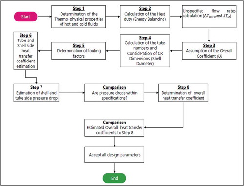
Figure 1. Methods used in this study

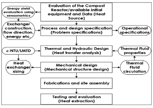
In Figure 1, the methods used in this study are shown, ranging from the Heat source (CR) evaluation to the testing and evaluation of the CR/COHE system. The site weather and geographical conditions were taken into consideration. The methods in the design of the proposed COHE were based on the engineering principles and methodologies outlined by (Abd & Naji, 2017; Bergman et al., 2011; Hayati, 2014; NPTEL, 2019; Shah & Sekulic, 2003).

2.1. Site geographical and climatic parameters

This study was carried out in Kitale, Trans-Nzia County in Kenya with a geographical location of Latitude 01° 08ʹ 39 N and Longitude of 034° 59ʹ48E. The study area is located at an average of 1907 m elevation, with mean annual temperature: maximum 26.4 °C and 12.3 °C minimum; average annual mean rainfall of 1259.1 mm with 85.6 sunshine hours per annum.

2.2. Experimental measures

The empirical data mining involved the measuring of temperatures, humidity, fluid flowrates, and the relative humidity at various points initially in CR and finally during the experimental trials (heat extraction) with COHE (Tube side) installed inside the CR (shell side).

2.3. CR physical properties evaluation

The compost feedstocks mixture and composition were as described (Mwape et al., 2020). Physical properties of the CR are important in ensuring an efficient aerobic composting system. The following were considered; Temperatures achieved Bulk density (BD_wet&dry), Particle size (diameter), Total Porosity (TP_or), Volumetric water content (V_wc), Free Air Space (FAS), Permeability (K), Superficial velocity (v), Permeability-based Reynolds number (Re) (dimensionless), Passibility (η), Pressure difference (ΔP), and Densities of ambient air and air Density in the CR. (H. M. Keener et al., 1993).

2.3.1. CR temperature profiles

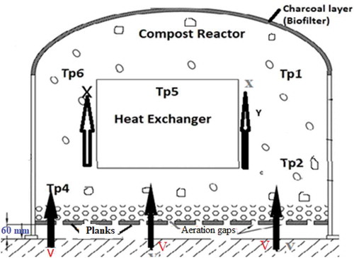
In this research setup, the source of energy was the heat from the CR. The aeration of the CR was statically achieved through the chimney effect created by the spaces left in between the wooden panels used at the ground stage of the CR as shown in Figure 2 which forced the air to move upward, resulting in a counter flow heat exchanger system. The air flowed upward as shown by the label V arrow in Figure 2. The CR was monitored and its temperature profiles analyzed. According to the tendance of natural convection, hot and moist air is pushed into the upper area of the CR; therefore, much heat is concentrated on the upper part (Seng et al., 2018). A condenser-type heat exchanger for CHRs designed and tested by (Bajko et al., 2019), was assembled on top of the compost reactor with consideration of the natural convection effect.

In Figure 2 Tp1 to Tp6 shows the Polytetrafluoroethylene (PTFE) thermocouples connected to the TC-8^TM Picolog Data loggers with a temperature accuracy of ±0.2% of reading and ±0.5 °C were used inside the CR to transmit the data to the PC via a 15 m USB cable. The PTFE were selected due to their robustness in withstanding the harsh conditions within CR due to humidity, pH changes, and microorganisms' actions resulting in a chemical reaction. Y denotes the corn stalk and the mixed compost feedstock in the compost reactor. Bajko et al. (2018), designed a wooden rod that was inserted into the Polypropylene to avoid corrosive environmental effects on the sensors.

T_p1 to T_p5 = thermocouples, x = Flow direction of water, V = Flow direction of heat

Figure 2. CR and COHE assembly with Thermocouple arrangement

2.3.2. CR fluid flow calculations

The aeration in passively aerated compost systems is governed by passive convection, resulting from subjecting a fluid of constant viscosity and not compressible, to a temperature gradient and is described by Darcy’s law. The force that drives the airflow is buoyant in nature and calculable by applying Archimedes principles. The buoyant force is said to be equal to the weight of the fluid been displaced (Das & Keener, 1997; Lynch & Cherry, 1996; Yu et al., 2006, 2009).

Average Air velocity; the following equation was used to calculate the average air velocity,

(1) $v=-\frac{K}{\mu }\frac{\mathrm{\Delta }P}{\mathrm{\Delta }\gamma }or-\frac{K}{\mu }\frac{\mathrm{\Delta }P}{L}=-\frac{K}{\mu }{\rho }_{Amb}g\left(1-\frac{T_{Amb}}{T_{CR1}}\right)$(1)

Where v = average air velocity (ms⁻¹), K = permeability of the compost (m²), ${\rho }_{Amb}$ = density of ambient air (kg m⁻³), $\mu$ = fluid dynamic viscosity of the air (m² s⁻¹), $T_{Amb}$ and $T_{CR1}$ = ambient and compost reactor temperatures, respectively, g = acceleration (9.8 m s⁻²), L = the length (m) of the occupancy of the porous medium. The fraction $\frac{\mathrm{\Delta }P}{\mathrm{\Delta }\gamma }$ = pressure gradient through the compost (Pa m⁻¹) (Yu et al., 2006). Equation 1(1) $v=-\frac{K}{\mu }\frac{\mathrm{\Delta }P}{\mathrm{\Delta }\gamma }or-\frac{K}{\mu }\frac{\mathrm{\Delta }P}{L}=-\frac{K}{\mu }{\rho }_{Amb}g\left(1-\frac{T_{Amb}}{T_{CR1}}\right)$(1) gives a linear relationship that exists between the steady velocity and the pressure gradient in laminar flow conditions only and ceases under the turbulent and transitional flow. High and above 1 Re, Darcy’s equation does not apply and the condition is no longer steady but turbulent (Notton, 2005; Siyu et al., 2005).

The density (${\rho }_{Amb}$) of the air was worked out using the Psychometric relationships since the temperatures of the ambient air, altitude (1900 m above sea level), and relatively humidity was conveniently measured as explained in the temperature capture section (ASHRAE, 2020). The thermal conductivity coefficient for the composting process is a function of its temperature and density of the feedstocks mixture. The higher the density, the higher the thermal conductivity of the compost reactor (Klejment & Rosiński, 2008). Consequently, the density of the CR is a function of its mass and the space it occupies (volume) (Jain et al., 2019).

The value of the airflow velocity is key in efficient heat generation by supplying oxygen for the reaction of oxidation and by removing heat from the reactor. It is this requirement to remove extra heat that gives an opportunity of thermal energy capture in this study. There is a ceiling value on the aeration flowrate that succumbs to the non-continuous linear relation between the respiration activities and the airflow supply (Mejias et al., 2017).The higher the velocity, the higher the heat loss that can result in inhibition and the lower the velocity the lower the heat generation (Luangwilai et al., 2010).

Total airflow and velocity rates suggested during composting are 4.4 × 10⁻³ m³s⁻¹ & 0.028 ms⁻¹ by Rynk et al. (1992), 4.1 × 10⁻² m³s⁻¹ & 0.255 m s⁻¹ by Haug (1993), 5.5 × 10⁻³ m³s⁻¹ & 0.34 ms⁻¹ Keener et al. (1997), and 8.8 × 10⁻⁴ m³s⁻¹ and 0.006 ms⁻¹ (Notton, 2005).

In order to calculate the average air velocity using Equation 1(1) $v=-\frac{K}{\mu }\frac{\mathrm{\Delta }P}{\mathrm{\Delta }\gamma }or-\frac{K}{\mu }\frac{\mathrm{\Delta }P}{L}=-\frac{K}{\mu }{\rho }_{Amb}g\left(1-\frac{T_{Amb}}{T_{CR1}}\right)$(1) , figures of the compost substrates such as, permeability (K), air viscosity (μ), Temperatures ($T_{Amb}and{T}_{CR1}$) in the compost, bulk density, density of ambient temperature, and Free Air Space (FAS), must be worked out. The importance of all these parameters is key in enabling the estimation of the effect of one parameter on another (physical properties) are highlighted by (J. Agnew et al., 2003; J. M. Agnew & Leonard, 2003).

2.3.3. Determination of Permeability

Published results were applied to determine the permeability values under the compaction of the compost in the CR, in this study since it was beyond the scope. The permeability values were estimated based on the published values with related values of bulk density, moisture content, and the initial Free Air Space (FAS_o) in respect to the compaction effect (Das & Keener, 1997; Notton, 2005; Yu et al., 2006). This method was applied by (Yu et al., 2006) to develop a practical analytical model of airflow in a passively aerated CR.

The ideal Gas Law and Archimedes principles were applied to compare the buoyant force acting on the air to the temperature difference between the air in the CR bed and ambient air. This was achieved under the assumptions of constant viscosity and negligible compressibility (H. K. Ahn et al., 2008; Siyu et al., 2005; Tiquia, 2005; Yu et al., 2006, 2009).

Darcy’s law was used to describe the creeping flow of the fluid that is not compressed and passing through a porous CR and is used under less than 1 Reynolds number (Re) (Yu et al., 2006).

2.3.4. Reynolds number and Pressure drop

The equations applied were:

(2) $Re=\frac{{\rho }_{CR}v\sqrt{K}}{\mu }<1$(2)

(3) $\mathrm{\Delta }P=({\rho }_{amb}-{\rho }_{CR})gH$(3)

Where Re = Reynolds for flow in a porous medium,$\mathrm{\Delta }P$= the pressure (Pa) deference driving force from the point of air entry into the CR until exist,${\rho }_{amb}$ and ${\rho }_{CR}$ = density (kg m⁻³) of ambient and inside compost reactor air, g and H are gravitational acceleration (9.8 m s⁻²). H = the height of the compost reactor after feedstocks loading (m), $v$ = average velocity of air, K = the permeability values, and $\mu$ = viscosity of the air.

2.3.5. Density

The density of the air at each point was calculated using:

(4) ${\rho }_{amb}and{\rho }_{CR}=\left[\frac{P_{da}}{\left(R_d\times T\right)}+\frac{P_{pv}}{\left(R_v\times T\right)}\right]$(4)

Where ${\rho }_{amb}and{\rho }_{CR}$ ambient and CR air density, respectively, $P_{da}$ = is the pressure of dry air (Pa), $P_{pv}$ = water vapour pressure (Pa), T (T_amb = 18.2 °C, T_CR = 66.8 °C) = air temperature in ^oC, $R_d$ = is the specific gas constant for dry air (287.058 J/(kg ^oC) and $R_v$ = specific gas constant for water vapour equal to 461.495 J/(kg ^oC) (OC, (Omni Calculator sp. zo.o.), 2020).

2.3.6. Free Air Space (FAS) determination

The equation linking the physical parameters is as stated below as recommended and used by (Agnew et al., 2003; Agnew & Leonard, 2003; Das & Keener, 1997; McCartney & Chen, 2001; Mejias et al., 2017; Siyu et al., 2005; Yu et al., 2006), was applied in this study.

(5) $FAS=100-BD\left[\frac{MC}{{\rho }_w}+\frac{100-MC}{PD}\right]$(5)

Where Free Air Space (%) = FAS, Bulk Density (wet basis (wb)) in (kg/m³) = BD, Moisture Content (wb) (%) = MC, the density of water (999 kg/m³) = ${\rho }_w$, and Particle density (kg/m³) = $PD$. The equation is applicable when all variables are known. All other particles are easily worked out apart from particle density (Agnew et al., 2003).

2.3.7. Bulk density (%) (BD)

The bulk density in this study was measured at different pile levels (depth) using the mass per unit volume technique.

Dry and Wet Bulk Density (BD_dry) (kg/m³): The dry bulk density was calculated using the following equation:

(6) $B{D}_{dry}=\frac{Weightofdrysolidsinthefeedstocks}{volumeofthecompostreactor}$(6)

(7) $B{D}_{wet}=\frac{MassofwetfeedstockintheCR}{Volumeofthereactor}$(7)

2.3.8. Total Porosity (TP_or)

The total porosity was workout using the following equation:

(8) $T{P}_{or}=1-\left(\frac{B{D}_{dry}}{{\rho }_p}\right)\times 100$(8)

2.3.9. Volumetric water content of the feedstocks

The volumetric water content of the feedstock matrix was calculated using (Agnew & Leonard, 2003):

(9) $V_{WC}=\frac{MC\times B{D}_{wet}}{{\rho }_w}$(9)

Given; $B{D}_{dry}andB{D}_{wet}$= dry and wet bulk density, respectively, of the feedstocks used in this experiments (kg m³), $V_{WC}$ = volumetric water content of the compost feedstocks (m³ m⁻³), $T{P}_{or}$ = Total porosity, ${\rho }_w$ = density of water (999 kg m⁻³), and ${\rho }_p$ = particle density of the feedstocks (Das & Keener, 1997).

2.3.10. Relationship between FAS, ${\mathit{V}}_{\mathit{W}\mathit{C}}$, and$\mathit{T}{\mathit{P}}_{\mathit{o}\mathit{r}}$

Das and Keener (1997) related the FAS, $T{P}_{or}$, and $V_{WC}$ using the following equation which was applied in this study:

(10) $FAS=T{P}_{or}-V_{WC}$(10)

2.3.11. Moisture Content (%)(MC wb) Water density and Free Air Space relationship with BD

Moisture contents were worked out before mixing of the feedstocks to retain a 58% MC wet basis and C:N of 28.8:1 gravimetrically at the Kenya Agriculture and Livestock Research Organization (KALRO), using the methods utilized by Agnew & Leonard (2003) and as highlighted in (Mwape et al., 2020). The C/N and pH ratios are as recommended to optimize the microbial action (Irvine et al., 2014, May; M. M. Smith & Aber, 2014).

Density of water (${\mathit{\rho }}_{\mathit{w}}$) (kg m⁻³): density of water at standard conditions of 999 kg m⁻³ was adopted.

Free Air Space (FAS): In this study, the general regression equation which is equivalent to the FAS equation term from Equation 5(5) $FAS=100-BD\left[\frac{MC}{{\rho }_w}+\frac{100-MC}{PD}\right]$(5) , $\left[\frac{MC}{{\rho }_w}+\frac{100-MC}{PD}\right]=0.09\pm \mathrm{0.001.}$ The following regression equation was used to work out FAS:

(11) $FAS=100-0.09B{D}_{wet}$(11)

Equation 11(11) $FAS=100-0.09B{D}_{wet}$(11) was used by (Agnew et al., 2003) and assumes a constant particle density at all moisture contents under any given compressive force. The relationship between the bulk density and FAS of composting materials is linear (Yu et al., 2009).

2.3.12. Particle density (kg/m³) $\mathit{P}\mathit{D}$ and Permeability (K)

The mean particle density used in this study was 1350 kg m⁻³ adopted from the ranges as indicated in Table 1 of (Das & Keener, 1997, p. 276).

Table 1. Design parameters of the Compost reactor (Shell side)

Design parameters	Units
Total Feedstock weight (kg) wb	1350.2
Moisture content (%)	58
Moisture content (kg)	779.4
Total weight (volatile solid matter & air) (db) (kg)	570.8
Initial (packed CR) depth in compost (d1) (m).	0.85
Final (Composted CR after 205 hrs) in compost (df) (m)	0.45
Particle Density (kg m^3) (Das & Keener, 1997)(J. M. Agnew & Leonard, 2003)	1350
Area based on (d1 =0.85) (m^2)	12.43
Volume based on (d1) (m^3)	2.4
Area based on (d2 =0.45) (m^2)	8.37
Volume based on (d2) (m^3)	1.3
Density of water (${\rho }_w$) (kg m^−3)	999
Thermal conductivity coefficient (Wm^−1oC^−1) (R. R. Zhao et al., 2015)	0.30
C/N ratio	28.8:1
pH	6.8
Average (Cp) (kJ/kg/^oC)	3.03
Average Initial Temperature (TCR1) (^oC)	65.56
Average Final Temperature (TCR2)(^oC)	53.33
Mass Flow rate (kg/s)	0.055
Heat Capacity (kW/^oC)	0.1666

Permeability (K): In this study, the relationship based on the physical characteristics of the feedstocks used was utilized to calculate the airflow parameters such as permeability using Ergun (1952)’s work that related the permeability (K) and the possibility (η), that are derived from the Kozeny-Carman model equation (Das & Keener, 1997; Richard et al., 2004; Siyu et al., 2005).

(12) $K=\frac{d\begin{array}{c}2\\ p\end{array}}{A}\times \frac{FA{S}^3}{{\left(1-FAS\right)}^2}$(12)

(13) $\eta =\frac{d_p}{B}\times \frac{FA{S}^3}{{\left(1-FAS\right)}^2}$(13)

Given, K and η = permeability (m²) and passibility (m), respectively. $d_p$ = particle diameter (m) which is an effective particle diameter (weighted average surface to volume ratio) (Macdonald et al., 1979) was measured at KALRO (0.0155 m), A and B = Ergun viscous component constant and inertial component constant, respectively (A = 180 and B = 1.8) as revised by Macdonald et al. (Richard et al., 2004).

Air volumetric and mass flow rate: Since the volumetric flow of air through a porous media (compost feedstocks inclusive), assumably flows in accordance to Darcy’s law, provided the pore flow velocities remain low and maintain the laminar flow, the volumetric flow was calculated in this study using (Lynch & Cherry, 1996; Poulsen & Moldrup, 2007):

(14) $\dot{\mathrm{V}}=\frac{KA\mathrm{\Delta }P}{\mu L}\left(m^3/s\right)\mathrm{a}\mathrm{n}\mathrm{d}\dot{\mathrm{m}}=\frac{KA\rho \mathrm{\Delta }P}{L\mu }\left(kg/s\right)$(14)

Where $\dot{\mathrm{V}}$ is the volumetric flow rate (m³ s⁻¹), K is permeability (m²), A is cross-section area of the CR (m²), $\mathrm{\Delta }P$ = pressure drop, L is length over which pressure drop is taking place, $\mu$ is viscosity of the air, and ρ is air density.

With all the physical parameters such as temperatures for the CR (T_CR1 and T_CR2) and COHE (water inlet T_COHE1), density, specific heat capacities, mass flow rates, etc., known, calculating the design parameters followed.

2.4. COHE Thermal Fluid Flowrates

The catch and weigh method was used for measuring the flowrates. A two hundred and fifty millilitres (250 ml) bottle was used and the time taken to fill it up measured on 10 runs basis to find the average. This method was used by (Burleson et al., 2020), during the computational modeling and empirical analysis of a biomass-powered drinking water pasteurization technology.

Two Mini DC 12 V 3 M micro submersible brushless water pumps with 5 watt consumption rated at 240 l/hr static flow, were used.

Polyethylene (PE) foam insulation material tightly wrapped around the fittings and connections between the compost reactor and the Water Tank (WT), improved heat insulation. One thermocouple mounted inside the supply pipe from the pile to the WT, monitored the temperature of the water.

The average water temperature was monitored and viscosity and density considered assuming a not more than 45 °C temperature rise.

2.4.1. COHE Surface Area

The surface area of the COHE was to be within the ratio of 1.5:1 to 3:1 (CR/COHE). This was to conform to the data reviewed from the literature were different researchers monitored, utilized the hydronic systems within these ranges (Compost mould/Core ratio) (Biomeiler, 2020; Pitschel & Lowry, 2016; Spade, 2014).

2.5. COHE mathematical modeling (design calculations)

The Kern’s method (Donald, Q Kern, 1983) and the engineering principles presented by Shah and Sekulic (Shah & Sekulic, 2003) and used by Irvine, were applied to design the COHE used in this study. Further, the step by step design procedures for the heat exchanger outlined and used by different designers were followed (NPTEL, 2019; Shawabkeh, 2015). The process and procedure adopted are shown in Figure 3.

Figure 3. COHE design procedure based on Kern’s methods (Abd & Naji, 2017; Hayati, 2014; Towler & Sinnott, 2013)

2.5.1. STEP 1: Thermal and hydraulic design

2.5.1.1. Thermal design

Thermal design of a heat exchanger involved the consideration of many interacting design parameters summarized as process and mechanical parameters.

2.5.1.2. Process parameters

The process parameters considered are as follows:

• Thermal fluid assignments to CR, which was the hot side (shell side), and the COHE which was the cold side.

• Average temperature specifications selection derived from the CR experimentation and water.

• Setting CR (shell side) and COHE (tube side) pressure drop design limits.

• Determination of heat transfer techniques and fouling coefficients for CR (shell side) and COHE (tube side).

The properties considered for the design for the water, CR Feedstock (FS), and the transport medium are: temperature flow rate (ṁ) (kg s⁻¹/kg hr⁻¹), density (kg m⁻³) and specific heat capacity C_p (kJ kg^−1oC⁻¹) (for water and the CR) and the thermal conductivity of (k_w) of 0.50 W m⁻¹ °C⁻¹ (ET, (Engineering ToolBox), 2011). The property details for the water and CR average C_p, and the HDPE are presented in Table 1 and Table 2 on the results sections, respectively. These were considered at the caloric temperature (Kern, 1983; NPTEL, 2019).

Table 2. Physical parameter Calculation Results

Parameters	Equ.	Units	Quantity
Bulk density $(\mathit{B}{\mathit{D}}_{\mathit{w}\mathit{e}\mathit{t}}$) @ d1	7	kg m^−3	562.58
Bulk density ($\mathit{B}{\mathit{D}}_{\mathit{d}\mathit{r}\mathit{y}}$) @ d1	6	kg m^−3	237.83
Particle size (diameter) measured at KALRO		m	0.0155
Total Porosity ($\mathit{T}{\mathit{P}}_{\mathit{o}\mathit{r}})$	8	%	82.38
Volumetric water content$\hspace{0.17em}({\mathit{V}}_{\mathit{W}\mathit{C}}$)	9	m^3 m^−3	32.63
Free Air Space (FAS)	5, 10&11	%	49.56
Permeability (K)	12	µm^2	6265.63
Superficial velocity (v)	1	m s^−1	0.024
Permeability based Reynolds number (Re) (dimensionless)	2		0.991
Passibility (η)	13	m	0.004
Pressure difference (ΔP)	3	Pa	1.99
Density—ambient air	4	kg m^−3	1.20
Mass flow rate	14	kg s^−1	0.055
Density-CR air	4	kg m^−3	0.96

2.5.2. Fouling factors determination

The fouling factor (R_wf) considered in this study was 0.002 m^{2 o}C W⁻¹ (town hard water) (Hayati, 2014; Hesselgreaves et al., 2017).

2.5.3. Determination of the Thermal Fluid

2.5.3.1. COHE (Tube side)

The thermal fluid used in the COHE was water due to its availability at a lower cost and the good thermal properties, good enough to absorb and store thermal energy (Allen & Chambers, 2009).

2.5.4. STEP 2: Energy Values evaluation (Energy balance)

Since the CR inlet and outlet temperatures, specific heat capacity, and mass flowrates, were known, it was easier to calculate the missing parameters for the COHE (outlet temperature of the water (T_COHE2)). The inlet water average temperature (T_COHE1) was evaluated prior to the tests.

2.5.4.1. Heat duty

Heat duty is the amount of energy the heat exchanger must transfer to the fluid used in the process to heat or cool to the required temperature. In this study, it involved the heat lost by the hot fluid (the CR) denoted by Q_CR and the heat gained by the cold fluid (COHE water) denoted by Q_COHE.

The principals of the law of conservation of energy complimented by the first law of thermodynamics were used to compare the energy generated by the shell side (CR) and assumed that it was gained by the tube side (COHE) (Zohuri, 2018), because energy is neither created nor destroyed. Previous researchers worked out the energy balance in heat exchangers using this method (Bergman et al., 2011; Irvine et al., 2014, May; Sekulic, 2020; M. M. Smith & Aber, 2014) and is expressed as:

(15) $Q_{CR}=Q_{COHE}$(15)

Where Q_CR was the heat energy lost by the CR and Q_COHE was the heat energy gained by the COHE. It should be noted that in this study, no phase change occurred; therefore, the formula used is for sensible heat transfer (Shah & Sekulic, 2003) and the analysis was subject to the following assumed conditions (Theodore, 2011):

• The heat exchange is only between the hot and cold thermal fluids (Insulated heat exchanger)

• Neglecting the axially conduction along the tubes

• Energy changes (potential and kinetic) were negligible

• Under constant specific heat capacities of thermal fluids in the CR and COHE

• Under constant overall heat transfer coefficient

• No phase change

Heat lost by CR

(16) $Q_{CR}={\dot{\mathrm{m}}}_{CR}C{p}_{CR}\left(T_{CR1}-T_{CR1}\right)$(16)

Where Q_CR is the total heat lost by the CR (kW), ${\dot{\mathrm{m}}}_{CR}$ is the mass flowrate of the CR in kghr⁻¹ heat stream underpinned by the moist air (0.055 kg/s or 198 kg/hr); Cp_CR is the average specific heat capacity of the feedstocks used in the CR (3.03 kJ kg⁻¹ °C⁻¹). (T_CR1—T_CR2) is the temperature difference between the initial (T_CR1) (65.56 °C) average highest temperatures attained during standalone CR tests to the average lowest assumed to avoid CR inhibition (T_CR2) 53.33 °C.

Heat gained by the COHE: From equation 16(16) $Q_{CR}={\dot{\mathrm{m}}}_{CR}C{p}_{CR}\left(T_{CR1}-T_{CR1}\right)$(16) , the energy lost by the CR was assumed to be the energy gained by the COHE as shown in Equation 17(17) $Q_{COHE}={\dot{\mathrm{m}}}_{COHE}C{p}_{COHE}\left(T_{COHE2}-T_{COHE1}\right)$(17) :

(17) $Q_{COHE}={\dot{\mathrm{m}}}_{COHE}C{p}_{COHE}\left(T_{COHE2}-T_{COHE1}\right)$(17)

Where Q_COHE is the total heat gained by the COHE (kW), ${\dot{\mathrm{m}}}_{CR}$ is the mass flowrate of the COHE in kg hr⁻¹ heat stream underpinned by the moist air (0.025 kg s⁻¹ or 90 kg hr⁻¹); Cp_COHE is the specific heat capacity of the water in the COHE (4.175 kJ kg⁻¹ °C⁻¹). (T_COHE1—T_COHE2) is the temperature difference between the initial (T_COHE1) (23.36 °C) and the calculated T_COHE2. The Mass flowrate (${\dot{\mathrm{m}}}_{COHE}$), Cp_COHE and the T_COHE1, of the COHE were known and therefore it was easier to work out T_COHE2 from Equation 17(17) $Q_{COHE}={\dot{\mathrm{m}}}_{COHE}C{p}_{COHE}\left(T_{COHE2}-T_{COHE1}\right)$(17) (Haug, 1993) and applied by G. Irvine, using the standard heat flow into a material with constant pressure.

2.5.5. STEP 3: Estimation of Overall heat transfer coefficients for the Tube (COHE) and Shell side (CR)

In this study, the range of the initial assumed overall heat transfer coefficient (OHTC) U_ass, was 11.34 W m⁻² °C (Appendix A), considered the moist air at low pressure from the CR as the hot fluid and water inside the tubes as the cold in a cooler type heat exchanger (Edge, 2020; Sinnott, 2005). The assumed OHTC was in line with the recommendation for low-pressure coolers with fluids at atmospheric pressure, liquid outside or inside and (gas) moist air at low pressure inside or outside the tubes in a cooler type heat exchanger (Edge, 2020; Sinnott, 2005). The assumed OHTC was within the 30% threshold recommended Kern’s limitations and used by Abd et al. (Abd & Naji, 2017; Kern, 1983; Towler & Sinnott, 2008). The OHTC assumed was in line with the ranges achieved by previous researchers (Mudhoo & Mohee, 2007; Sylla Boundou et al., 2006).

This process was key in helping in calculating the area values using the mean temperature difference (Abd & Naji, 2017). The overall heat transfer coefficient depends on the tube side (COHE) and the shell side (CR) individual heat transfer coefficients and fouling resistances (Dhavle et al., 2018; ET, (Engineering ToolBox), 2003; Kern, 1983).

2.5.6. STEP 4: Determination of the tentative CR (shell)-COHE (Tube passes-n_p)

In this step the tentative number of shell (CR) and tube (COHE) passes (n_p) and the Log mean Temperature deference (LMTD) and its correction factor (F) were determined. For the steady and efficient operation of the heat exchanger, the (F), was to be higher than 0.75 (Donald, Q Kern, 1983; NPTEL, 2019). In this study, one shell and multiple tube pass configuration were considered.

2.5.6.1. Logarithmic Mean Temperature Difference (LMTD)

The LMTD just like the Effectiveness equation is specific to the heat exchanger fluid flow direction (Bergman et al., 2011). The following equation was used to find the LMTD:

(18) $LMTD=\frac{{\theta }_2-{\theta }_1}{lo{g}_e\frac{{\theta }_2}{{\theta }_1}}$(18)

For counterflow, the LMTD was given by:

(19) ${\theta }_1=T_{CR1}-T_{COHE2},{\theta }_2=T_{CR2}-T_{COHE1}$(19)

In addition, for the Parallelflow, the temperatures were worked out using:

(20) ${\theta }_1=T_{CR1}-T_{COHE1},{\theta }_2=T_{CR2}-T_{COHE2}$(20)

In this research, the counterflow arrangement was selected.

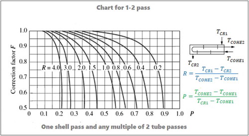
2.5.6.2. Log-mean Temperature Difference Correction Factor F

The correction factor (F), is the ratio of the True (effective) Mean Temperature Difference (TMTD) (ΔT_m) to the LMTD and referred to as the log-mean temperature difference correction factor, or exchanger configuration factor. This can also be found by the ratio of the actual heat transfer rate of a heat exchanger to that of a Counterflow heat exchanger with equal UA and fluid terminal temperatures.

F is dimensionless and dependents on the effectiveness of the temperature, heat capacity ratio, and the direction of fluid flow of the heat exchanger in consideration (Shah & Sekulic, 2003). The chart for one to two shell pass and two, four, six (multiples of 2) tube passes (Appendix B) was used to configure and compare the mathematically calculated F. To compare, the two dimensionless temperature ratios were calculated as follows:

(21) $R=\frac{T_{CR1}-T_{CR2}}{T_{COHE2}-T_{COHE1}}$(21)

And

(22) $S=\frac{T_{COHE2}-T_{COHE1}}{T_{CR1}-T_{COHE1}}$(22)

The above equations for R and S were also applied to calculate the Heat Exchanger Thermal Efficiency (HETE) where the relationship of ε and NTU data was used for conditional flow arrangements. These methods entailed the calculation of the dimensionless parameters S and R, which are determinants of the correction factor (F) by using the following equations.

F was given by:

(23) $F=\frac{\mathrm{\Delta }{T}_m}{\mathrm{\Delta }{T}_{Im}}=\frac{q}{UA\mathrm{\Delta }{T}_{Im}}$(23)

Where TMTD was calculated using:

ΔT_m = F ΔT_LMTD

Or

(24) $\mathrm{\Delta }{T}_m=\frac{\mathrm{\Delta }{T}_{max}\epsilon }{NTU}=\frac{T_{CRIN}-T_{CROUT}}{\frac{UA}{C_{CR}}}=\frac{T_{COHEOUT}-T_{COHEIN}}{UA/C_{COHE}}$(24)

2.5.6.3. Heat capacity rates

Individual thermal fluid heat capacity rates were worked out using;

(25) $C=\dot{\mathrm{m}}{C}_p$(25)

Where C is the fluid heat capacity, $\dot{\mathrm{m}}$ is the mass flow rate of the fluids and C_p is the specific heat capacities of the fluids. In this study C_min was C_COHE standing for the heat capacity of the COHE and C_max, was the heat capacity of the CR.

Heat Capacity ratio (C*) was given by;

(26) $C\ast =\frac{C_{min}}{C_{max}}$(26)

2.5.7. Step 5 Heat transfer determination

The energy calculated in step 2 using Equation 16(16) $Q_{CR}={\dot{\mathrm{m}}}_{CR}C{p}_{CR}\left(T_{CR1}-T_{CR1}\right)$(16) , relates with the heat transfer area, Overall Heat Transfer Coefficient selected in step 3 and the T_m in Equation 24(24) $\mathrm{\Delta }{T}_m=\frac{\mathrm{\Delta }{T}_{max}\epsilon }{NTU}=\frac{T_{CRIN}-T_{CROUT}}{\frac{UA}{C_{CR}}}=\frac{T_{COHEOUT}-T_{COHEIN}}{UA/C_{COHE}}$(24) .

(27) ${\mathit{Q}}_{\mathit{C}\mathit{R}}={\mathit{Q}}_{\mathit{C}\mathit{O}\mathit{H}\mathit{E}}=\mathit{U}\mathit{A}\mathrm{\Delta }{\mathit{T}}_{im}$(27)

(28) $A_o=\frac{Q}{\left(U\mathrm{\Delta }{T}_m\right)}=\pi {\mathit{d}}_{\mathit{o}}\mathit{L}$(28)

Where Q is the total heat transfer rate, U_ass is overall heat transfer Coefficient (Wm⁻²K⁻¹), A_o is the total heat transfer area (m²) and T_m is the log-mean Temperature Difference, d_o is the outside diameter of the tube and L is the length of the pipe in meters (LMTD) (Abd & Naji, 2017; Ezgi, 2012).

2.5.8. Step 6:Pipe sizing and material determination

The size selected was 0.01905 m OD (d_o) with a wall thickness of 0.003 m and ID (d_i) of 0.01605 m HDPE and 2.143 m long per turn on the Hydronic heat exchanger frame. The BWG sizing was achieved using (USAI, (USA Industries), 2020).

2.5.8.1. Length of the Pipe (L)

The length of the pipe was worked from Equation 28(28) $A_o=\frac{Q}{\left(U\mathrm{\Delta }{T}_m\right)}=\pi {\mathit{d}}_{\mathit{o}}\mathit{L}$(28) as follows:

(29) $L=\frac{A_O}{\pi d_o}$(29)

2.5.8.2. Number of tubes

The number of tubes required to cover the heat transfer area (A) was calculated using;

(30) ${\mathit{n}}_{\mathit{t}}=\frac{\mathit{A}}{\mathit{\pi }{\mathit{d}}_{\mathit{o}}\mathit{L}}$(30)

2.5.8.3. Outside surface area of one turn of the tube on the exchanger, frame (A_ot)

(31) $\left(A_{ot}\right)=2.143\times \pi d_o$(31)

Where 2.143 = L is the length of one turn of the pipe on the frame and d_o = outside diameter of the HDPE pipe.

2.5.8.4. Number of turns on the heat exchanger frame

(32) $Numberofturns\left(N_t\right)=\frac{A_o}{A_{ot}}$(32)

Where A_o is the provisional total outside surface area of the tubes and A_ot is the outside surface area of one turn of the tube.

2.5.8.5. Diameter of the pipe bundle and pitch

(33) $p_t=1.25d_o$(33)

(34) $D_b=d_o{\left(\frac{N_t}{K_1}\right)}^{\frac{1}{n_1}}$(34)

D_b = bundle diameter in m, p_t = pitch, d_o = tube OD in m, N_t = number of turns, K₁ and n₁ are constants from the number of passes and triangular pitch.

The constants K₁ and n₁ were obtained from the pitch coefficients table (Appendix C) obtained from (Dhavle et al., 2018; N. Shah, 2020; Shawabkeh, 2015).

2.5.8.6. Selection of the clearance between the shell side and the bundle

In this study, the fixed and U-tube were chosen from the bundle and shell diameter chart in Appendix D (Abd & Naji, 2017). The shell diametrical clearance was selected and applied in the calculation of the clearance of bundle diameter as follows:

(35) $D_s=\mathrm{B}\mathrm{u}\mathrm{n}\mathrm{d}\mathrm{l}\mathrm{e}\mathrm{D}\mathrm{i}\mathrm{a}\mathrm{m}\mathrm{e}\mathrm{t}\mathrm{e}\mathrm{r}\mathrm{c}+\mathrm{c}\mathrm{l}\mathrm{e}\mathrm{a}\mathrm{r}\mathrm{a}\mathrm{n}\mathrm{c}\mathrm{e}$(35)

2.5.8.7. Heat transfer coefficient—Tube side

The average thermal conductivity of water (0.62 W/m^oC) between 20 °C (0.59 W/m^oC) and 50 °C (0.65 W/m^oC) was used in this study. Thermal conductivity of water increase linearly with temperature (Ramires et al., 1995).

Mean temperature of the water was worked out;

(36) $meanwatertemperature=\frac{T_{COHE2}+T_{COHE1}}{2}$(36)

Total flow cross-section area of the tube in this study was worked out using;

(37) $A_{at}=\frac{\pi }{4}{d_i}^{2}X{N}_t\left(m^2\right)$(37)

A_at = total flow cross-sectional area.

Water mass velocity (G_t);

(38) $Velocity\left(G_t\right)=\frac{\dot{m}}{A_{at}}\left(\frac{kg}{s{m}^2}\right)$(38)

Water linear velocity (u_t);

(39) $u_t=\frac{G_t}{\rho }\left(m{s}^{-1}\right)$(39)

OR

(40) ${\mathit{u}}_{\mathit{t}}=\frac{4\dot{m}\left({\mathit{n}}_{\mathit{p}}/{\mathit{n}}_{\mathit{t}}\right)}{\pi \mathit{\rho }\mathit{d}\begin{array}{c}2\\ \mathit{i}\end{array}}$(40)

Reynolds number;

(41) $Re=\frac{\rho u_t{d}_i}{\mu }$(41)

Where $\dot{m}$ = mass flowrates (kg s⁻¹), $\rho$ = density (kg m⁻³) and μ = viscosity in cp (NPTEL, 2019).

Water Coefficient: the following equation given from the data of (Eagle & Ferguson, 1930) was used in this study to calculate the water coefficient;

(42) ${\mathit{h}}_{\mathit{i}}=\frac{4200\left(1.35+0.02\mathit{t}\right){\mathit{u}}^{0.8}}{{{\mathit{d}}_{\mathit{i}}}^{0.2}}\mathit{O}\mathit{R}\frac{{\mathit{h}}_1{\mathit{d}}_{\mathit{i}}}{{\mathit{k}}_{\mathit{f}}}={\mathit{j}}_{\mathit{h}}\mathit{R}\mathit{e}\mathit{P}{\mathit{r}}^{0.33}{\left(\frac{\mathit{\mu }}{{\mathit{\mu }}_{\mathit{w}}}\right)}^{0.14}$(42)

Where h_i = water coefficient-inside (W m^−2oC), t = water temperature (^oC), u_t  = water linear velocity (m s⁻¹), d₁ = inside tube diameter (m), k_f = conductivity of the fluid (W m^−2oC), Re = Reynolds number (dimensionless). Pr = Prandtl number (dimensionless), μ = viscosity of water (0.0008 Ns m⁻²), j_h = heat transfer factor from (Sinnott, 2005, p. 665), and μ_w = viscosity of the water at wall temperature (N s m⁻²).

Prandtl number calculations;

(43) $\mathit{P}\mathit{r}=\frac{{\mathit{C}}_{\mathit{p}}\mathit{\mu }}{{\mathit{k}}_{\mathit{f}}}$(43)

K_f = 0.62 W m⁻¹ °C

Finding the heat transfer factor: The heat factor for this study was worked by dividing the pipe length (L) in m by the internal diameter (ID) (d_i) in m:

(44) $\frac{\mathit{L}}{{\mathit{d}}_{\mathit{i}}}$(44)

The tube side heat transfer factor table was used to find the heat transfer factor (Abd & Naji, 2017; Sinnott, 2005, p. 665).

2.5.8.8. Heat transfer coefficient-Shell side (CR)

Baffle Spacing: the baffle spacing (l_b) used was selected to be as close as possible to give higher heat transfer coefficients (Hayati, 2014; Kern, 1983).

Determination of cross-flow area: The cross-flow area (A_s) of the hypothetical row at the middle of the shell (equator), was calculated by:

(45) $A_s=\frac{\left(p_t-d_o\right)D_s{l}_b}{p_t}$(45)

A_s = cross-flow area, p_t = tube pitch depicted by distance between centers of two tubes (P_t = 1.25d_o), d_o = tube outside diameter (m), D_s = diameter of the shell inside (m), l_b = baffle spacing (m).

Determination of mass (G_s) and linear (u_t) velocity of the shell side:

(46) $G_s=\frac{W_s}{A_s}$(46)

And,

(47) $U_S=\frac{G_S}{\rho }$(47)

W_s = fluid flow rate (kgs⁻¹) on the shell side, ρ = density of the fluid in the shell side (kgm⁻³).

Determination of the hydraulic diameter (shell equivalent diameter): the formula used was:

(48) $d_e=\frac{4\left(\frac{p_t}{2}X0.87p_r-\frac{1}{2}\pi \frac{{d_o}^2}{4}\right)}{\frac{\pi d_o}{2}}=\frac{1.10}{d_o}\left(p_t^2-o.917d_o^2\right)$(48)

Where d_e = equivalent diameter (m) (Hayati, 2014; Kern, 1983).

Average CR (shell side) temperature:

CR mean temperature:

(49) $\left(CR\right)=\frac{T_{CR1}+T_{CR2}}{2}$(49)

Reynolds number:

(50) $Re=\frac{\rho u_s{d}_e}{\mu }=\frac{G_s{d}_e}{\mu }$(50)

CR Prandti number (Pr):

(51) $P_r=\frac{C_p\mu }{k_f}$(51)

(52) $Nu=\frac{h_s{d}_e}{k_f}=j_{h}ReP{r}^{\frac{1}{3}}{\left(\frac{\mu }{{\mu }_w}\right)}^{0.14}\left(minustheviscositycorrectionterm\right)$(52)

Finding the j_h by choosing the 25% baffle cut from the shell-side heat transfer factor graph (Hayati, 2014, p. 36) (Shawabkeh, 2015).

Finally, the shell side (CR) heat transfer coefficient was calculated by:

2.5.9. STEP 7: Pressure drop

The equation offered for calculating the pressure drop was:

Tube side

(53) $\begin{array}{rl}& \mathrm{\Delta }{P}_t=N_p[8j_r\left(\frac{L}{d_i}\right){\left(\frac{\mu }{{\mu }_w}\right)}^{-m}+2.5]\frac{\rho u_t^2}{2}\\ & \left(neglectingviscositycorrectionterm\right)\end{array}$(53)

Or,

$\mathrm{\Delta }{P}_t=8j_r\left(\frac{D_s}{d_i}\right)\left(\frac{L}{l_b}\right)\frac{\rho u_t^2}{2}{\left(\frac{\mu }{{\mu }_w}\right)}^{-0.14}$

Where L = tube length

$l_b=\mathrm{b}\mathrm{a}\mathrm{f}\mathrm{f}\mathrm{l}\mathrm{e}\mathrm{s}\mathrm{p}\mathrm{a}\mathrm{c}\mathrm{i}\mathrm{n}\mathrm{g}$

Find j_r from the tube side friction factor graph (Hayati, 2014, p. 39) using the Re number found in Equation 41(41) $Re=\frac{\rho u_t{d}_i}{\mu }$(41) (Kern, 1983).

Shell side:

(54) $Linearvelocity=\frac{G_s}{\rho }$(54)

Then used the Re in Equation 50(50) $Re=\frac{\rho u_s{d}_e}{\mu }=\frac{G_s{d}_e}{\mu }$(50) to find the j_r from the shell side friction factor segmental baffles graph (Hayati, 2014, p. 40; Kern, 1983).

Pressure drop was given by:

(55) $\mathrm{\Delta }{P}_t=8j_r\left(\frac{D_s}{d_s}\right)\left(\frac{L}{L_s}\right)\frac{\rho u_s^2}{2}$(55)

2.5.10. STEP 8: Overall heat transfer coefficient

The overall heat transfer coefficient of the COHE pipe was calculated by adding the stand-alone heat transfer coefficients of the thermal fluids involved using

(56) $\frac{1}{U_o}=\frac{1}{h_o}+\frac{1}{h_{od}}+\frac{d_{o}ln\left(\frac{d_o}{d_i}\right)}{2k_w}+\frac{d_i}{d_i}X\frac{1}{h_{id}}+\frac{d_o}{h_{id}}X\frac{1}{h_i}$(56)

Where o = outside pipe wall (m), i denotes the inside of the pipe wall (m), and U represents the overall heat transfer coefficient (W m^{−2 o}C⁻¹).

(57) $\mathrm{i}\mathrm{f}0<\frac{U_{o,Calc}{U}_{o,assum}}{U_{o,assum}}<30\mathrm{\%}\mathrm{t}\mathrm{h}\mathrm{e}\mathrm{n}\mathrm{a}\mathrm{s}\mathrm{s}\mathrm{u}\mathrm{m}\mathrm{e}\mathrm{d}{U}_o\mathrm{i}\mathrm{s}\mathrm{c}\mathrm{o}\mathrm{r}\mathrm{r}\mathrm{e}\mathrm{c}\mathrm{t}(\mathrm{N}\mathrm{P}\mathrm{T}\mathrm{E}\mathrm{L},2019)$(57)

2.6. Experimental setup (Mechanical structure design and Fabrication)

Mechanical Parameters: The mechanical parameters considered were:

• The COHE Tubular Exchanger Manufacturers Association (TEMA) layout and the number of passes.

• Tube parameter specifications (size, layout, pitch, and material).

• Lower and upper limits on the length of the tube.

• CR parameters (average feedstocks C_p, area, volume, flowrates, and density).

• Design parameters of the CR.

It should be noted that the system was designed to operate at a steady state (Edwards, 2008; Sekulic, 2020; Sölken, 2020).

This section addressed the fabrication of the exchanger based on the mathematical calculations achieved. Fabrications were done according to the design drawings depicting the mathematical calculations and presented in Figure 4. The heat source fluid (air) was influenced by a passively aerated system that moved from the bottom to the top based on the chimney effect as shown in Figure 2. The CR design and functions are based on (Mwape et al., 2020).

Figure 4. Front view of the COHE

In Figure 4, the Cold fluid (water) flow direction is shown. It entered the COHE from the top and flowed back to the water tank through the bottom. The water, therefore, flowed in a counter direction to the Heat source resulting in a Counterflow heat exchanger (Theodore, 2011).

2.7. Performance Analysis Formulation

In this study, the performance indicators of the COHE were performed using the ε-NTU method (Theodore, 2011). To compare the Temperature efficiency between different heat exchangers such as, counterflow, crossflow, and parallelflow the, Log Mean Temperature Difference (LMTD) method was applied. These methods were used by (Adumene et al., 2016). Further step by step heat exchanger design aspects were followed (Edwards, 2008; Shawabkeh, 2015).

2.7.1. Effectiveness of the COHE

The effectiveness of the COHE was worked out using the heat exchanger effectiveness equations that are specific to the heat exchanger fluid flow direction. In this study, the counterflow system was used, based on the flow of the fluids in the CR/COHE system. This method was also adopted by and covered widely.

(58) $\epsilon =\frac{Actualheattransfer}{Maximumpossibletransfer}=\frac{Q}{Q_{max}}$(58)

Where $\epsilon$ is the effectiveness of COHE, Q is actual heat transfer, and Q_max is the maximum possible heat transfer. Equation 59(59) $Q=1exp\left[-NTU(1-C{ }^{\ast })\right]$(59) is further identified by the following equations:

(59) $Q=1exp\left[-NTU(1-C{ }^{\ast })\right]$(59)

Where C* is heat capacity ratio expressed in Equation 25(25) $C=\dot{\mathrm{m}}{C}_p$(25) .

In addition, Q_max is simplified in the following equation:

(60) $Q_{max}=1-C{ }^{\ast }exp\left[-NTU(1-C{ }^{\ast })\right]$(60)

Equation 60(60) $Q_{max}=1-C{ }^{\ast }exp\left[-NTU(1-C{ }^{\ast })\right]$(60) and 61(61) $\epsilon \frac{Q=1exp\left[-NTU(1-C)\right]}{Q_{max}=1-Cexp\left[-NTU(1-C)\right]}$(61) results in the effectiveness of the counterflow with the equation;

(61) $\epsilon \frac{Q=1exp\left[-NTU(1-C)\right]}{Q_{max}=1-Cexp\left[-NTU(1-C)\right]}$(61)

The final calculation was to find the COHE water outlet temperature using the following equation:

(62) $\epsilon =\frac{C_{CR}\left(T_{CR1}-T_{CR2}\right)}{C_{min}\left(T_{CR1}-T_{COHE1}\right)}=\frac{C_{COHE}\left(T_{COHE2}-T_{COHE1}\right)}{C_{min}\left(T_{CR1}-T_{COHE1}\right)}$(62)

2.7.2. Number of Transfer Units (NTU) and Temperature Correction Factors

The NTU was given by;

(63) $NTU=\frac{UA}{C_{min}}$(63)

Where U_ass is the overall heat transfer coefficient, A_o is the area of the heat transfer surface, C_min minimum heat capacity between the thermal fluids, and NTU is the Number of Transfer Units (Shah & Sekulic, 2003).

The association of the LMTD and ε-NTU was key in carrying out assumptions using P and R values to calculate heat capacity ratio (C*) Equation 25(25) $C=\dot{\mathrm{m}}{C}_p$(25) and effectiveness equation 61(61) $\epsilon \frac{Q=1exp\left[-NTU(1-C)\right]}{Q_{max}=1-Cexp\left[-NTU(1-C)\right]}$(61) . If R ˂ 1, R = heat capacity ratio (C*) Equation 25(25) $C=\dot{\mathrm{m}}{C}_p$(25) , and P = ε (equation 61(61) $\epsilon \frac{Q=1exp\left[-NTU(1-C)\right]}{Q_{max}=1-Cexp\left[-NTU(1-C)\right]}$(61) and equation 62)(62) $\epsilon =\frac{C_{CR}\left(T_{CR1}-T_{CR2}\right)}{C_{min}\left(T_{CR1}-T_{COHE1}\right)}=\frac{C_{COHE}\left(T_{COHE2}-T_{COHE1}\right)}{C_{min}\left(T_{CR1}-T_{COHE1}\right)}$(62) .

The above assumptions were used by (Guimaraes et al., 2015) in the numerical determination of the LMTD correction factor for shell and Heat Exchangers. They are further illustrated by (Shawabkeh, 2015)

2.7.3. Effectiveness and NTU relationship

The ε-NTU relationship for the counterflow (Equation 61(61) $\epsilon \frac{Q=1exp\left[-NTU(1-C)\right]}{Q_{max}=1-Cexp\left[-NTU(1-C)\right]}$(61) ), crossflow (single pass) both fluids unmixed (CF(sp)BFU) (Equation 65(65) $\epsilon =1-exp\left[\left(\frac{1}{C^{\ast }}\right){\left(NTU\right)}^{0.22}\left\{exp\left[-C^{\ast }{\left(NTU\right)}^{0.78}\right]-1\right\}\right]$(65) ) and Parallelflow (equation 64(64) $\epsilon =\frac{1-exp\left[-NTU\left(1+C^{\ast }\right)\right]}{1+C^{\ast }}$(64) ) at known NTU and C*, were evaluated using the different effectiveness equations as follows (Theodore, 2011):

• Parallel flow

(64) $\epsilon =\frac{1-exp\left[-NTU\left(1+C^{\ast }\right)\right]}{1+C^{\ast }}$(64)

• Crossflow (single pass) both fluids unmixed

(65) $\epsilon =1-exp\left[\left(\frac{1}{C^{\ast }}\right){\left(NTU\right)}^{0.22}\left\{exp\left[-C^{\ast }{\left(NTU\right)}^{0.78}\right]-1\right\}\right]$(65)

The objective was to evaluate the heat exchangers with the better ε under the standard NTU and C*.test conditions used in this study.

2.8. Statistical methods

Temperature profiles were captured by means of the Polytetrafluoroethylene (PTFE) thermocouples connected to the TC^TM-8 Picolog Data loggers with a Temperature accuracy of ±0.2% of reading and ±0.5 °C, were used to transmit the data to the PC via a 15 m USB cable. The PTFE thermocouples were chosen because of the robustness to withstand harsh conditions within CR due to humidity, pH changes, and microorganisms actions resulting in chemical reactions. Bajko et al. (2018), designed a wooden rod that was inserted into the Polypropylene to avoid corrosive environmental effects on the sensor. Testo 174 H and FreeTec data loggers as were also used to capture data.

The temperature data were then downloaded to the PC and using OriginPro 2018, which uses many nonparametric tests such as Friedman ANOVA and two-sample Kolmogorov-Smirnov test to confirm the normality of the data P values range (P˂0.005).

2.9. Computational Model

The Chemical Engineering Calculations Hydronic Compost Heat Exchanger design and performance evaluation software here referred to as HYDROCOHE software was created to be used in this study. A computation model was created in the CheSheets a free web-based spreadsheet program developed by the Chemical Engineering Calculations (CheCal) and distributed on an as-is basis and free software, that provides step by step guidelines on designs of a chemical engineering system. A Google sheet was developed and coded to return output values based on specified input parameters under the Compost reactor situation using the Visual Basic for Applications (VBA) skills (Chelcal, 2018).

The HYDROCOHE input values were based on the Fluid and the Exchanger data. The Fluid data composed of flowrates, Hot-for CR (ṁ_CR) and Cold for COHE (ṁ_COHE), input temperatures (T_CR1 and T_COHE1) and the specific heat capacities (C_pCR and C_PCOHE). In the exchanger data, the type of the fluid flow arrangement was considered (Counterflow, parallelflow, and crossflow all fluids unmixed) and the overall heat transfer Coefficients (U).

The outputs were based on the calculations coded using VBA from the mathematical equations discussed in this study, and the outlet temperatures, (T_CR2) and (T_COHE2). The calculations achieved were; the heat transfer conductance, the NTU, the Effectiveness (ε), the heat capacity ratio (C*), Heat transfer or energy rate (Q), the mean temperature difference (MTD), the LMTD, and the LMTD Correction factor (F). The outlet temperatures obtainable were for the CR (T_CR2) and the COHE (T_COHE2). The ε-NTU curves were done.

The default model was predicating initially on counterflow direction values. During the comparison tests, the input configuration was changed to the crossflow and parallelflow heat exchangers flow sets. The results of each heat exchanger’s performance were correlated with each other, with the mathematically obtained values.

2.10. Computation and Empirical values Comparisons

After experimental trials of the CR and COHE assembly, the average temperature, flow, and energy values obtained, where simulated into the HYDROCOHE system to output the values and compare. This was important to validate the experiment and the data obtained.

2.11. Ethics statement

The collection of the samples was permitted by the owners of the farm in the Malidadi area of Kitale at the geographical location of Latitude 01° 08ʹ 39 N and Longitude of 034° 59ʹ48E and elevation 1907 m. The chicken manure (CM) and the sawdust (SD) were voluntarily provided by a local chicken farmer and sawmill owners, respectively. The National Commission for Science, Technology, and Innovation (NACOSTI), a Government statutory board in Kenya, issued the research license number NACOSTI/P/18/99,643/27,086. Therefore, all experimental procedures conformed to the regulations established by the NACOSTI.

3. Results and discussion

3.1. Experimental analysis of the CR

The design and achieved parameters of the CR used in this study are presented in Table 1 and Table 2 summarizes the calculated physical parameters.

3.1.1. Summary of feedstocks and CR parameters

The feedstocks used are, cow manure, green farm weeds, maize cobs as bulking materials, maize stovers, and sawdust. The C/N and C_p calculations are highlighted in (Mwape et al., 2020). The quantities and physical parameters are as summarized in Table 1.

The composting process is controlled by environmental factors (temperature, pH, moisture content, and aeration) and Feedstocks/substrate natural factors (C/N ratio, nutrient content, and particle size) (Diaz et al., 2007; Makan et al., 2014). Therefore, most importantly, in this study was the balancing of the heat generation from the compost reactor and the efficiency of the heat-loving microorganisms responsible for aerobic composting stabilization. Previous studies list heat release as an indication of the aerobically composting process stability and are directly associated to the air supply for the process of aeration (Notton, 2005).

The physical properties considered in this study and highlighted by other researchers are highlighted in Table 2 (Agnew et al., 2003; Agnew & Leonard, 2003; Notton, 2005; Walling et al., 2020). Air supply to the composting system has threefold functions; Oxygen supply line to the micro-organisms, excess moisture removal, and the dissipation of excess heat generated (Diaz et al., 2007; Makan et al., 2014; Notton, 2005). The design and achievement of a good quantity of air supply and its efficiency is linked to a complete understanding of the physical properties, processes, and materials involved.

The temperatures achieved were in the range of 66.8 and 18.4 ^oC maximum in the CR and ambient, respectively. The ambient air density calculated was 1.20 kg m⁻³. Upon entering the CR and at the maximum temperature of 66.8 °C, the air density calculated was 0.96 kg m⁻³. This reduction of density as the result of the heat generation from the microbial activities causes the air to rise (weight reduction) to the top leaving a space thereby creating the chimney effect, that aids the inflow of air from the bottom of the CR. Furthermore, the condensate was observed on CR top plastic cover, signaling the condensation of the evaporated water from the compost which further points to air density reduction, thereby exacerbating airflow (Poulsen, 2013).

The drop in density from 1.20 to 0.96 kg m⁻³ in this study, created a pressure difference of 1.99 Pa. Airflow rate is further affected by the permeability (Barrington et al., 2002; Das & Keener, 1997). Achieved in this study was a permeability of 6265.63 µm², which is in the range of the reported ranges of 2500–25,000 µm² and 700–8000 µm² for biosolids and cow manure, respectively, over a compressive pressure stress ranging between 0 and 20 kPa. Air permeability is important in that it is indirectly proportional to the stress exerted on the CR (J. M. Agnew & Leonard, 2003).

The air porosity achieved in this study was 82.38% and was good enough to allow the airflow resistance decrease and permitted the flow and was in the range of the reported and recommended (J. M. Agnew & Leonard, 2003). At 82.38% porosity, the CR was provided with enough air and water-filled voids to allow adequate water and air availability to ensure efficient microbial activities at the particle size of 0.0155 m. This resulted in the FAS of 49.56% that is in accordance with the reported values, good enough to command easy air and water flow through the CR feedstocks and had great influence on the heat and mass transport, and microbial kinetics (Alburquerque et al., 2008).

The permeability (K) is dependent on the FAS and the particle size as shown in Equation 12(12) $K=\frac{d\begin{array}{c}2\\ p\end{array}}{A}\times \frac{FA{S}^3}{{\left(1-FAS\right)}^2}$(12) . The superficial velocity also depends on the fluid kinemics viscosity of the air as shown in Equation 1(1) $v=-\frac{K}{\mu }\frac{\mathrm{\Delta }P}{\mathrm{\Delta }\gamma }or-\frac{K}{\mu }\frac{\mathrm{\Delta }P}{L}=-\frac{K}{\mu }{\rho }_{Amb}g\left(1-\frac{T_{Amb}}{T_{CR1}}\right)$(1) . The superficial velocity achieved in this study was 0.024 m s⁻¹ and a mass flow rate of 0.0055 kg s⁻¹. Similar figures have been reported (Alkoaik et al., 2019).

The achieved parameters in this study qualified the flow described by Darcy’s law since the Reynolds number was less than 1 (0,991) (Poulsen, 2013; Siyu et al., 2005; Yu et al., 2006). The good temperature profiles achieved, were good enough to proceed with heat extraction through the designing of the COHE.

It should be noted that trials on the operation of the Compost reactor were conducted separately before the extraction process was instituted and not reported here. The heat bulb (Exchanger) thermal fluid used was water. The storage water tank was 36 liters capacity and raw water from the Kitale water utility company used. The CR with the above parameters was the heat generator.

3.1.2. Summary of achieved CR and COHE thermal fluids experimental parameters

The initial average temperatures (Input) for the CR (moist air) and COHE fluids achieved were 65.53 °C and 23.36 °C, respectively. In order to prevent the cooling of the CR, the minimum temperature drop expected was 53.33 °C. The assumed overall heat transfer coefficient (U_ass) was 11.34 and was in line with the recommendation in Appendix A (Low-pressure coolers), liquid outside or inside and (gas) moist air at low pressure inside or outside the tubes in a cooler type heat exchanger (Edge, 2020; Sinnott, 2005). The assumed OHTC was within the 30% threshold recommended Kern’s limitations and used by Abd et al (Abd & Naji, 2017; Kern, 1983; Towler & Sinnott, 2008).

Upon having the CR and COHE thermal and flowrates parameters, designing calculations were possible and results are presented below.

3.2. Mathematical methods

In Table 4, the cold and hot side physical parameters achieved, are presented.

Table 3. Cold and Hot fluid physical parameters

PARAMETERS		SHELL SIDE DATA	TUBE SIDE DATA
1	Mass flowrate (kg hr^−1)	198	90
2	Inlet temperature TCR1/TCOHE1 (^oC)	65.56	23.36
3	Outlet temperature TCR2/TCOHE2 (^oC)	53.33	42.89
4	Inlet pressure (psi)	14.7	1.4
5	Fouling allowance (m^2 °C W^−1)	0.002	0.00035
PHYSICAL PROPERTIES (AVERAGE)
1	Temperature (^oC)	59.45	33.12
2	Specific heat (CpCOHE/CpCR) (kJ kg^−1 °C)	3.03	4.175
3	Thermal conductivity (k) (W m^−1 °C)	0.30	0.65
4	Density (kg m^−3)	1.13	999
5	Viscosity (cp) (Ns m^−2)	0.0198	0.8
HEAT BALANCE
1	Energy (QCR = QCOHE) (kWh)		7337.27
2	Power (kW)		2.038
3	Assumed Overall Heat Transfer Coefficient (Uass)		11.34

Table 4. Heat exchanger design calculations

CALCULATIONS AND DIMENSIONLESS PARAMETERS
LMTD (^oC) = 26.15	R = 0.626	S = 0.289	F = 0.9566	LMTD corrected = 25.02 °C
				P = 0.464
ESTIMATED LAYOUT
Materials	CR =Biomass feedstocks		COHE = HDPE
Tube OD (m) = 0.01905	Tube Length (m) = 2.143	Pitch =0.024	Shell pass = 1	Tube pass = 56	Tube ID (m) = 0.01605
NUMBER OF TUBES
Ao (m^2) = 7.2	Area of 1 tube (m^2) = 0.128	Number of tubes pass = 56 Number of shell pass = 1		Number of Tubes per pass = 1
Tube cross-section area (m^2) = 1.445*10^−5		Volumetric Flowrate (m ^3 s^−1) = 2.5*10^−5	Tube side Velocity = (m s^−1) = 1.73	Water mass velocity (kgs^−1m^2) = 0.0035
BUNDLE & SHELL DIAMETER
k1 = 0.215	n1 = 2.207	Bundle Diameter (Db) (m) = 0.237
Bundle-shell clearance (m) = 1.60		Shell Diameter = 1.84
TUBE SIDE HEAT TRANSFER COEFFICIENT
Reynolds # = 51,609.93	Prandtl # = 13.47	Length Diameter ratio = 133.62	Nusselt # = 486.96	Jh Factor = 0.004	h1(Wm^−2 °C) =18,204.34
BAFFLE SPACING &SHELL SIDE VELOCITY
Baffle Spacing (m) = 0.74	As = 0.27	Volumetric Flowrate (m^3 s^−1) = 0.049		Shell Side velocity (m s^−1) = 0.18
SHELL SIDE HEAT TRANSFER COEFFICIENT
Equivalent Dia (De) (m) = 0.019	Reynolds Number = 23.8		Prandtl # = 0.486	Jh Factor = 0.0075	hs (W m^−2 °C) = 13.96
CALCULATED OVERALL HEAT TRANSFER COEFFICIENT
Thermal conductivity (kw) (W m^−1 k^−1) = 0.5			Uo (W m^2 °C) = 13.48
Tube side Pressure Drop Pt (psi) = 0.085			Shell side pressure drop Ps (psi) = 0.12

3.2.1. Energy balance

An energy balance for the two fluids (Shell =CR and Tube = COHE) was achieved using Equation 16(16) $Q_{CR}={\dot{\mathrm{m}}}_{CR}C{p}_{CR}\left(T_{CR1}-T_{CR1}\right)$(16) . It was assumed that heat loss to the surrounding was negligible, with no potential or kinetic energy changes, no phase, and specific heat capacity changes, and at steady-state conditions (Kuppan, 2000; Mujumdar, 2007). The data and results used to perform the energy/heat transfer and calculated T_COHE2 is presented in Table 4.

3.2.2. Design and Performance analysis using Kern and ε-NTU/LMTD methods

The design and performance analysis was achieved by using Kern and ε-NTU methods (Abd & Naji, 2017; Towler & Sinnott, 2013). The inlet temperatures were 65.53 °C for the CR (T_CR1) and 23.36 °C for the COHE (T_COHE1).

3.2.2.1. Mechanical Design: Type of heat exchanger and dimensions

In this study, a one-shell pass and 56 tube passes counterflow heat exchanger arrangement, was adopted. The LMTD method was applied to calculate the required area of the COHE and detailed results are presented in Table 5.

Table 5. Summary Design parameters of the COHE

Parameter	Values
Mass flow rate of the fluid (H2O) (kg s^−1)	0.025
Volume of the COHE (m^3)	0.036
Length of Pipe (m)	120 m
Thermal conductor	Water
Auxiliary system energy Consumption (kW)	0.01 kW(12DCV)
Average Initial Temp. (TCOHE2) (^oC)	23.36
Average Max. Temp (TCOHE1) (^oC)	42.88
Specific heat Capacity (kJ kg^−1 °C^−1)	4.175
Pipe outside surface Area (m^2)	7.2
Heat capacity (CCOHE) (kW ^oC^−1)	0.1044

As indicated, the correction factor (F), was 0.9566, above 0.75 recommended for steady operation of the heat exchanger, thereby validating the efficiency of the configuration applied in this study (Ali & Naji, 2017; Kern, 1983; NPTEL, 2018; Towler & Sinnott, 2013)

The layout used in this study is outlined in Table 5 (0.01905 m-OD and 0.01605 ID). The thermal conductivity of the material used in this study (HDPE) 0.50 W/m/^oC, was lower than the ones in metals such as copper (385 W/m/^oC) or steel (50.2 W/m/^oC) (ET, (Engineering ToolBox), 2011). The higher the thermal conductivity of a material, the better the conduction of heat (Theodore, 2011).

The actual heat transfer area (A_o) was 7.2 m². It was noted in this study that increasing the overall heat transfer coefficient resulted in the reduction of the required total heat surface area of the heat exchanger. Abd and Naji (2017), indicated that the reduced heat transfer area in heat exchanger designing, translates into reduced equipment costs for both manufacturing, fouling, and maintenance costs. In a heat exchanger like this one where the shell side was the heat generator also depending on the microorganisms through composting, care was taken to ensure that the COHE/CR area ratio was not below 1.5 to avoid inhibition.

4. Tube and Shell side parameters Analysis

The tube side fluid velocity calculated in this study was 1.73 ms⁻¹ at the Re number of 51,609.93, resulting in a turbulent flow. On the other hand, the shell side velocity was 0.18 ms⁻¹ at the Re of 23.8 qualifying it into a laminar flow. For Re ˂ 2100 is laminar flow, 2100˂Re˂10,000 is transitional and Re ˃10,000 is turbulent flow (Theodore, 2011, p. 288).

The baffle size used in this study was 25% cut which is widely used and within 0.2 D_s. All dimensionless figures were considered as highlighted in the methodology section and Table 2.

The shell side (CR) heat transfer coefficient achieved in this study was 13.96. Previous studies have reported heat transfer coefficients in the range of 13.55, 17.50, 17.46, and 23,95 W m⁻² °C⁻¹ (Sylla Boundou et al., 2006). Mudhoo and Mohee (2007) reported that the overall heat transfer coefficients during composting of organic substrates aerobically are proportional to the temperatures. (The higher the temperature the higher the OHTC.) They found maximum OHTC between 35.5 and 263.9 W m⁻² °C⁻¹, and minimum between 2.44 and 8.15 W m⁻² °C⁻¹. Consequently, the tube and shell side heat transfer coefficients were calculated resulting in the overall transfer coefficient of 13.48, 18.9% of the assumed, and within the recommended 30% (Bergman et al., 2011; Kern, 1983; NPTEL, 2019). The pressure drops were also within the required ranges making the calculations valid for further tests and validation.

4.0.3. Summary of COHE design parameters

The summarized design parameters for the COHE are shown in Table 5 and were used in the fabrication works.

4.1. Fabrication and site assembly

The COHE was fabricated following the parameters in Table 5. The HDPE pipe was weaved onto the frame that acted as a baffled stage as shown in Figure 5. It was inserted into the CR as presented in (Mwape et al., 2020).

4.2. Experimental Methods-Performance Analysis

4.2.1. Experimental Set-up

The experimental set-up was achieved using the parameters and procedures explained in (Mwape et al., 2020).

4.2.2. Energy and Temperatures Values achieved

4.2.2.1. Temperature profiles

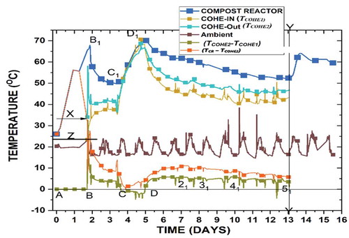
The temperature profiles achieved by the CR and COHE are shown in Figure 5. On day 1.88, 60 °C was achieved, the highest of 68.9 °C (Point B₁) recorded from a starting point of 25.5 °C. This temperature/duration achievement was reported by (Shimizu, 2017) who achieved similar values in 2–4 days. Similarly (Allen & Chambers, 2009) reported 65 °C while composting Horse-based manure from an in-vessel tunnel composting facility in Scotland.

The extraction of heat from the COHE started on day 1.88 when on average, CR was at 65.56 °C, water in the tank (T_COHE1) at Z was 23.36 °C, T_COHE2 at X, was 33.9 °C and the ambient was 20.06 °C. A to B (T_COHE2—T_COHE1), was at Zero before extraction started. Upon switching on the water circulation pump, the T_COHE2 went up to 58.1 °C. This jump in temperature rise is attributed to the reserve water that was in the COHE system (34-liter volume). The water in the tank went up 35.1 °C at this level. However, within 5 hours of extraction commissioning, the temperatures sharply went down to 40.4 °C in the COHE (T_COHE2), 33.7 °C in the water tank and 61.9°C in the CR, attributing the drop to the hot and cold water mixing. Between day 1.88 and 3.5, the temperatures remained constant between 40.1 ^oC snf 42 ^oC in the T_COHE2and 30°C and 38 °C in the T_COHE1.

The temperatures from the COHE went down from 41 to 36.2 ^oC by 07:28 am on day 3.6. At these time set the T_COHE1 temperature was at 34.9 °C, ambient was 16°C and around an average of 51 °C from the compost reactor.

Figure 5. Average temperature profiles used for energy calculations

Allen and Chambers (Allen & Chambers, 2009), reported similar temperature drops where an initial activation of the heat extraction using a compost heat extractor with the fluid mixed with water and Glycol was used to heat the water from 5 ^oC to 48 °C, but dropped to 38 °C after 5 minutes. This signified that more heat has been extracted than what has been generated by the CR. This is the critical problem associated to the heat extraction systems as also reported by (Bajko et al., 2018) and was addressed by staggering the extraction rates and times.

To mitigate on the temperature drop of the in the setup, a 400/750 watts electric water heater procured locally, was introduced to the water tank to heat the system above 55 °C, a temperature recommended for the good composting process. Heating started at point C₁ in Figure 6 and continued for 37 hrs 29 minutes until the water tank attained 70.1 °C. The compost average temperature rose to 69 ^oC. The maximum COHE_IN temperature was 70.1 °C and 68.7 °C for the COHE_OUT, minimum of 23.4 and 33.9 °C, respectively. The total energy used by the electrical heater was 28.1 kWh.

4.2.3. CR/COHE and T_COHE1/T_COHE2 Temperature differences

In Figure 6, the average temperature differences between the T_COHE2 and T_COHE1, and T_CR and the T_COHE2, are indicated. Points A and B indicate the period before extraction commenced and the difference between T_COHE2 and T_COHE1 was Zero. CR was above 65 °C. Areas C and D show the period when the electrical heater was operational. The net temperature was negative because the cold fluid (T_COHE1), supplied more heat than the T_CR. Upon turning off the electrical water heater at point D, the pattern of having the positive value for temperature difference resumed. The average difference temperature throughout the heat extraction period between the T_COHE2 and T_COHE1 4 °C and between the T_CR and T_COHE2, was 8.5 °C with the maximum and minimum of 32.5 and 31.7 °C and −4.5 and—0.12 °C, respectively.

Figure 6. Temperature differences between COHE_out & CR and COHE_OUT & COHE_IN.

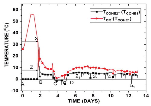
The ambient temperature was 14.6 °C average. Points 2₁–5₁ show the effects of solar irradiance on good sun days. The water tank received more heat from the sun resulting in a negative temperature between the T_COHE2 and T_COHE1. This was also experienced and highlighted by (Allen & Chambers, 2009).

The analyzed temperature values are in agreement with a section of the approved and existing research work and therefore are credible enough to be applied for the subsequent energy calculations.

4.2.4. Generated and Extracted energy

Extracted energy increased to727 MJ (201.94 kWh) during the extraction trials for 205 hours representing 17.83% of the total generated energy (4,077.4 MJ). The net extracted was 174 kWh (0.99 kW), minus the energy used by the electrical water heater of 28.1 kWh. This resulted into 7.8 kg/kWh or 538 kJ/kg per initial mass compost weight matter and 1273.65 kJ/kg on dry matter and 58,600 kJ/m². Similar extraction levels have been reported by (Seki & Komori, 1995) who extracted 54,550 kJ/m² representing 16–22% of 739,827.4 kJ generated using a lab-scale positive aerated cylindrical CR of diameter 0.58 m and height of 0.895 m. In this analysis, a small difference can be attributed to the poor thermal insulation of CR by a thin polypropylene fabric. Average recovery rates of 1159 kJ/kg dm for lab-sized systems, 4302 kJ/kg dm for pilot scale systems, and 7084 kJ/kg dm for commercial systems were presented (M. M. Smith et al., 2017). Therefore, the energy figures achieved in this study are not only reliable but also credible and comparable to other researchers.

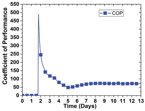
4.2.5. Coefficient Of Performance (COP) of COHE

The COP of the COHE during the Extraction period was a maximum of 489.9 and an average of 74.22 and gradually reduced to 71.5 on day 13 as shown in Figure 7 8. Zero COP was registered, during the first 1.74 days the COHE was not activated (No heat extraction). The average energy used by the pump throughout the trial period was 2.7 kWh.

The results are higher than (Allen & Chambers, 2009), where a maximum of 12.5 COP was achieved while extracting heat from the compost reactor using a Groundfos UPS 15–50 130ʹ flow pump rated at 55.2 w, 3.4 mhr⁻³ and 6 m maximum head as compared to the pump used in this setup of 5 w and 48 DCV power requirement. The different power consumption explains the difference in the COP. The less energy the auxiliary system uses (pumping/heating system), the higher the COP.

Figure 7. COP of the COHE during 205 hours heat Extraction

4.2.5.1. Performance evaluation

The performance analysis results are summarised in Table 3. The cooler fluids exist in counter flow heat exchangers, at the end of the system where the hot fluids join the heat. The hottest cold fluid temperatures greater than the coldest hot fluid temperatures have been reported in the counter flow heat exchangers as opposed to the parallel flow ones (Tawil, 1993).

The heat capacity rates of the heat source CR (C_CR) and the cold fluid COHE water (C_COHE) were 166.92 W/^oC and 104,375 W/^oC, respectively. The temperature of the cold fluid changed from 23.36 °C to 42.88 °C registering an increase of 19.52 °C as compared to the change of the hot fluid from 65.56 to 53.33 °C (Δ 12.23 °C). In this case, where the heat capacity rate of the Hot fluid is higher than the Cold fluid, it is highlighted that the cold fluid would absorb more heat hence larger temperature change (Theodore, 2011).

The effectiveness-NTU method was applied to analyze the heat exchanger in this study because only the inlet temperatures were known initially. This method is recommended by (Theodore, 2011) and (Shah & Sekulic, 2003) and was applied to design and evaluate a waste energy extraction system from the Composting facility located in Scotland, UK and recorded, ε of 0.7370, NTU of 1.5135. This method is simple than using the LMTD that requires prior knowledge of the inlet and outlet temperatures in order to calculate the T_IM.

If the heat capacity rate of the hot fluid source was less than that of the cold fluid, the hot fluid would have experienced the larger temperature change and cooled down to the cold fluid temperature (Theodore, 2011). This effect can cause the cooling down of the compost reactor from the thermophilic stage if the temperatures go below 45 °C due to microbial activities interference (Adams, 2005).

The capacity ratio (C*) was 0.6258 and was derived from dividing the smaller to larger heat capacity rate between the CR fluid and the COHE fluid and hence mass flow rate dependant. C*≤1 in this design. A balanced heat exchanger is one with C* =1. The fouling capacity (0.002 W/m²/°C) is the standard considered when dealing with a fluid with more than 50 °C temperature (R. K. Shah & Sekulic, 2003).

COHE effectiveness was 0.464. For specific U values and C_min, the value of NTU is the surface area configuration. It also represented the ratio of the actual heat transfer rate (2.038 kW) to the maximum possible heat transfer rate (4.404.625 kW) of the COHE. The larger the NTU, the larger the heat exchanger (Mohamad, 2015). The achieved effectiveness in this study is lower than the one reported in of 0.7270 at the actual heat transfer rate of 9889.3897 kW and a maximum possible heat transfer rate of 13,603.883 kW.

The F value found in this study was 0.9566 with a percentage relative error of −4.34% from the recommended unit F for a true counterflow exchanger with maximum temperature potential and with two fluids logically arranged in counterflow. T_m was 25.02 °C approaching the T_Im (26.15 °C) (R. K. Shah & Sekulic, 2003).

Therefore, 4.34% relative error represented the degree of departure of the TMTD from the LMTD and not a signal of high efficiency but an indication in the close operating performance of a heat exchanger with comparable operating conditions of flow rates and temperature inlets of the involved thermal fluids in a counterflow exchanger. Numerical correction factors for the LMTD for shell and tube 1–2 heat exchanger have been highlighted by (Guimaraes et al., 2015).

The LMTD of the Counterflow heat exchanger was 26.15 °C in this study (Equations 18(18) $LMTD=\frac{{\theta }_2-{\theta }_1}{lo{g}_e\frac{{\theta }_2}{{\theta }_1}}$(18) /19). Calculating at the attained input and output temperatures for the CR and the COHE. This would translate to 22.71 °C if a parallelflow heat exchanger was operated instead. This indicates that in the Counterflow heat exchanger, 26.15 °C was the mean difference in the temperatures between the COHE and the CR fluids. This indicates that the Counterflow heat exchangers transfer more heat than the parallelflow heat exchanger when operated under the same conditions. The LMTD correction was 25.02 °C.

4.3. Computation Analysis of the COHE

The input values used in the HYDROCOHE software were; inlet temperatures (T_CR1-65.56 °C), the (T_COHE1- 23.36 °C), CR flow rate (198 kg/hr), the COHE flowrate (90 kg/hr), the COHE area (7.2 m) and the overall heat transfer coefficient (11.34). The results are shown and discussed in section 3.4.1 where effectiveness comparative analysis of the three types of heat exchangers is explained. Figure 10 shows the input data and results.

Figure 8. Extract of the Computer program developed

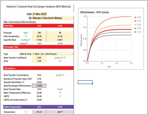
4.3.1. Comparison of heat exchangers effectiveness at a given NTU and C*

The achieved C* and NTU in this study was 0.626 and 0.79, respectively. Table 7 shows the comparative parameters of the parallelflow, counterflow, and crossflow heat exchangers at the achieved C* and NTU in this study.

Table 6. Performance parameters

Parameter	Symbol	Results
Heat capacity rates (W/^oC)	CR (CCR) (Cmax)	166.92
	COHE (CCOHE) (Cmin)	104.375
Heat capacity Ratio	C* =CMIN/CMAX	0.626
Heat transfer Coefficients (W/m^2/°C)	COHE	558.05
	CR	11.360
Fouling capacity (standard) (m^2 °C/W) (R. K. Shah & Sekulic, 2003).	Rwf	0.002
Number of transfer Units (NTU)	NTU	0.7499
Effectiveness (ε)	ε	0.464
	Q	0.2449
	Qmax	0.5279
Total pipe length	Surface area(m^2/m)	0.06
	Pipe length (m)	120

Table 7. Effectiveness at same NTU and C*

Exchanger	Equation #	NTU	C*	ε
Counterflow	61 a	0.7499	0.6253	0.464
^ZCF(sp)BFU	65	0.7499	0.6253	0.446
Parallelflow	64	0.7499	0.6253	0.433

^ZCrossflow (single flow) both fluids unmixed.

The objective of this section was to compare the heat exchangers in terms of the flow type that would achieve the highest Effectiveness.

Table 7 6 shows that at fixed NTU and C*, the ε of the Counterflow heat exchanger was 0.464, Crossflow (single flow) both fluids unmixed 0.446, and parallelflow was 0.433.

In Counter flow heat exchangers, the effectiveness is in the range of 0 ≤ε ≤1 (Bergman et al., 2011). The nearer the ε value to 1, the higher the energy, the heat exchanger transfers.

In Figure 11 –13, the modeling results of Effectiveness (ε)—NTU for the Counterflow, Crossflow (single flow) both fluids unmixed, respectively, are shown on the ε—NTU curves. In Figure 11–13 C_r = C*.

Figure 9. Effectiveness (ε)—NTU curves for Counterflow heat exchanger

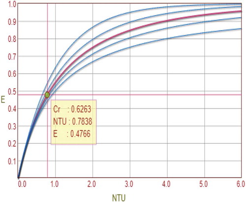
Figure 10. Effectiveness (ε)—NTU curves for Crossflow (Single flow) both fluids unmixed heat exchanger

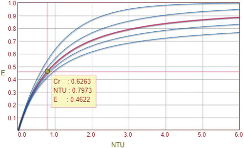
Figure 11. Effectiveness (ε)—NTU curves for parallelflow heat exchanger

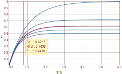
Table 8 shows the modeling results comparing the performance and behavior of the Counterflow; Crossflow (single flow) both fluids unmixed and parallel heat exchangers at the initial input temperatures (T_CR1 and T_COHE1).

Table 8. Effectiveness (ε)—NTU modeling results

Parameter	Types of Heat Exchangers
	Counter	^ZCF(sp)BFU	Parallel
Heat Capacity Ratio (C*)	0.6263	0.6263	0.6263
NTU	0.7838	0.7973	0.7838
Effectiveness (ε)	0.4766	0.4622	0.4430
Heat Transfer (Q) (kW)	2.10	2.02	1.95
Outlet hot fluid Temp-CR (^oC) (TCR2)	52.94	53.44	53.83
Outlet cold fluid Temp-COHE (^oC) (TCOHE2)	43.51	42.71	42.09

The Counterflow heat exchanger transferred 2.10 kW, at ε of 0.4766, T_CR2 of 53.94 °C and T_COHE2 of 43.51 °C. The CF(sp)BFU generated 2.02 kW at ε of 0.4622, T_CR2 of 53.44 °C and T_COHE2 of 42.71 °C. The parallelflow heat exchanger gave out 1.95 kW at T_CR2 of 53.83 °C, T_COHE2 of 42.09 °C, and at 0.4430 effectiveness.

Therefore, the following is the analysis and conclusion from the effectiveness (ε), NTU and C* relationship achieved in this study and charts highlighted by (Tawil, 1993):

• With small values of NTU up to about 1.5, the value of the effectiveness increase greatly. Effectiveness ranges from 0 to 1 and reduces with larger values of NTU (larger than 3). For example, at 3.0 NTU in Figure 13, the ε was 0.6, almost equal to ε at 6.0. Operating a heat exchanger with higher NTU (larger sized heat exchanger), is economically not feasible. This is because larger NTU does not translate into good effectiveness but a larger heat exchanger area.

• Comparatively, at a certain NTU and capacity ratio (C*), the highest effectiveness is registered by the Counterflow heat exchangers (0.4766 Figure 11) seconded by the cross-flow heat exchangers (both fluids unmixed) (0.4622 Figure 12). Parallelfow exchangers have the lowest effectiveness values (0.4430 Figure 13). Tables 7 and 8, through the mathematical and computational modeling have demonstrated this principle achieved in this study accurately.

• At NTU values below 0.3, the effectiveness of the heat exchanger is not dependent on the capacity ratio, as shown in Figures 11–13.

• At equal heat capacity rates of two fluids, the heat capacity ratio is 1 (boilers and condensers), the effectiveness is minimum. The maximum effectiveness is achieved at C* = 0 for a given NTU. C*, ranges between 0 and 1.

The larger the NTU number, the larger the size of the heat exchanger (Theodore, 2011).

4.4. Model Validation (Mathematical, Experimental, and Computational Analysis)

The Mathematical and computation analysis results between the Counterflow is here presented in Table 9. The average temperatures achieved using the HYDROCOHE compared to the Mathematical, had minor differences with an R² value of 0.99938 between the T_CR2 outlet temperatures and the R² value of 0.9995 between the outlet T_COHE2 temperatures. When validating the model, the difference between the experimental and predicted temperatures was considered by (Burleson et al., 2020) and adopted the R² value of 0.9992. Hence the range in this study is as what was previously applied, rendering this model valid.

Table 9. Mathematical, Empirical, and Computer simulations results based on counterflow arrangement

Parameter/Type of analysis	Math.	Comp.	Emp.	Difference (%)
Heat Capacity ratio (C*)	0.6253	0.6261	0.6253	0.128
NTU	0.7499	0.7528	0.2753	0.385
Effectiveness (ε)	0.464	0.4651	0.2248	0.237
Heat transfer (Q) (kW)	2.042	2.040	0.99	51.52
Total Heat Transfer Coefficient (U)	10.5777	10.532	3.883	0.432

Math =Mathematical modeling, Comp. = computer modeling and Emp. = Empirical modeling.

For the mathematical and HYDROCOHE software-computed values, the heat capacity ratio had the R² value of 0.9987, NTU registered R² of 0.9962, R² of 0.9976 for ε, and heat transfer (Q) had 0.9992 R² and the R² value of 0.9957 for the heat transfer coefficient. In the research to Optimize heat exchangers by a Bio-Inspired Artificial Intelligence Methods, J. Krzywanski used a maximum error lower than ± 3% to validate the approach (Krzywanski, 2019).

In this study, the error was between 0.1 and 0.4%, hence validated. Therefore, the presented procedure can be adopted as a technique in the heat exchanger design and performance analysis in the CHRs utilization systems. It is not only an effective method than the existing approaches, but also an alternative method for the existing trial and error CHRs heat exchanger design and optimization approaches that are complex analytically and numerically, and depends on unstandardized high costing experiments.

In the empirical data, the heat capacity ratio was not affected by the mathematically calculated, because the specific capacities between the CR and COHE fluids did not change and the mass flowrates assumed constant. However, the Overall Heat transfer coefficient dropped to 3.883 W/m²/°C giving a 0.3671 R² value. This explains why the energy extracted was giving an R² of 0.4848 compared to the mathematically calculated and the HYDROCOHE computed values. This can be attributed to the poor thermal conductivity between the CR feedstock materials (Huet et al., 2012, September) and the scaled & corroded LDPE piping surface due to the caustic environment created in the CR during composting as shown in Figure 12.

Figure 12. Scaled up and corroded COHE parts

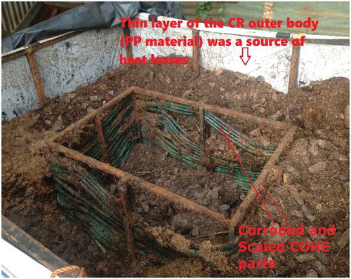
It is therefore deduced that the higher the overall heat capacity coefficients, the higher the heat transfer in a heat exchanger (Alkoaik et al., 2019).

Table 10 shows the comparison in the output temperatures between the T_CR2 and the T_COHE2 mathematically, computed and experimentally. The R² value between the Math and the Comp temperatures was 0.9993 and 0.9995 for the CR (T_CR2) and the COHE (T_COHE2), validating the tests. However, between HYDROCOHE and empirical, the R² values were 0.9269 & 0.9432, CR (T_CR2) & (T_COHE2), respectively. The CR fluid had higher outlet temperatures than the COHE fluid. This might backup the low extraction rate of the COHE experimentally. It can also be attributed to the high fouling rate of the COHE pipes and its lower thermal conductivity. Scientifically, when the transfer surface of the heat exchanger is fouled, the distance between the width of the two thermal fluids may be reduced and is correlated with reduced heat transfer rate and increased pressure drop (Theodore, 2011).

Table 10. Temperature comparisons (Mathematical, HYDROCOHE, and Empirical)

Parameter	Type of analysis	Mathematical.	HYDROCOHE.	Empirical.	(%) difference
Outlet Temp.	CR (TCR2)	53.33	53.297	57.5	7.252
	COHE(TCOHE2)	42.88	42.94	45.5	5.626

The power extracted experimentally was 0.99 kW as compared to the 2.10 kW computed by the HYDROCOHE and the calculated by the mathematical modeling of 2.042 kW. This is a difference of 51.47–51.52% (R² value of 0.4853–0.4848). This divergence between the simulation outcomes and the experimental values was observed by Nwanze and Clark (Nwanze & Clark, 2019), who by using a computer-based model in COMSOL Multiphysics^TM, discovered that the empirical data and the Simulation collated in the initial stages of the composting process, but diverged during the thermophilic stage. This was attributed to the heat losses of the compost reactors. Other researchers such as (Mohee et al., 1998), equally confirmed the rapid drop in temperatures during the thermophilic stage of the composting process, hence diverging from the computation setup.

Ventilative heat losses of 70–95% and 36–67% of the total heat flux in full and laboratory-scale compost reactors, respectively, due to conductive, radiation, and convective losses, have been reported by Mason and Milke (Mason & Milke, 2005).

The effects of insulation on the performance of compost reactors with rotary shape have been presented. It is highly recommended that for efficient and quality composting, insulation is effective and necessary for laboratory-scale and small pilot scale CRs with an Area/volume ratio of less than or equal to 6. This is because heat loss is high as A/V increases. The larger the compost piles, the lower the A/V ratio resulting in minimal heat losses (Alkoaik et al., 2019).

In this study, the A/V ratio was 4.4 and only a 3 mm Polypropylene cloth was used as insulation. The power discrepancy of 1,052 kW reported in this research between the empirical data, and the simulated and calculated data can therefore be attributed to the CR’s poorly thermal-insulated boundaries as depicted in Figure 12.

Further, low thermal conductivity coefficients of 0.31 W/m/^oC have been reported for a compost density of 600 kg/m³ at 60 °C and is dependent upon the moisture content, particle size, bulking agent quality and depth of the CR (H. Ahn et al., 2009). The more compacted the CR is, the higher the bulk density hence the higher the thermal conductivity coefficiency (Huet et al., 2012, September).

The CR used in this study had 201.7 kg/m³ density and within 60 °C, hence poor thermal conductivity coefficient cannot be ruled out, in contributing to the difference in the energy extracted.

5. Conclusions

The possibility of using the aerobic composting route of biomass wastes conversion to energy has been presented in this study and 175 kWh was extracted. Associated challenges to the designing of heat extraction systems from the CHRs and the mitigation are proposed by using the computer-based HYDROCOHE software. The relationship between the Hydronic compost heat exchanger’s mathematical and HYDROCOHE computer-based, design, and experimental performance modeling schemes was discussed in this paper. The mathematical and Computer-based produced similar results with R² values between 0.9962 and 0.9992 on the effectiveness, heat capacity ratio, NTU, heat transfer (Q), heat transfer coefficient, and outlet fluids temperatures (Hot and Cold fluids).

The Mathematical and the HYDROCOHE computer model have shown that the Counterflow heat exchanger arrangement, transfers more heat at the same design parameters (heat capacity rates, NTU, heat transfer coefficients, area, and inlet temperatures), than the crossflow and parallelflow heat exchanger arrangements. Since the generation of heat in the CHRs is heat-loving microorganisms-dependent, parallelflow, heat exchanger arrangements are highly recommended because of their ability to maintain the outlet temperatures at lower temperature differences as compared to crossflow and conterflow arrangements. Using the Counter or crossflow arrangements might result in the inhibiting of the compost system.

The conclusions drawn from the analysis of the data analyzed are:

• The computed effectiveness values from the CHECALC-based software and that realized from the actual empirical model, are almost the same.

• The heat generated by the CR (between 30 and 80 %) was lost via conduction, convection, and radiation.

• The CHECALC-based design software differed in terms of the experimental Outlet temperatures.

• At NTU values below 0.3, the effectiveness of the heat exchanger is not dependent on the capacity ratio, as shown in the Figure 9 to 11.

• At equal heat capacity rates of two fluids, the heat capacity ratio is 1 (boilers and condensers), the effectiveness is minimum. The maximum effectiveness is achieved at C* = 0 for a given NTU. C*, ranges between 0 and 1.

• The larger the NTU number, the larger the size of the heat exchanger.

• Using the LDPE as a piping material affected the heat capture rate because of its lower thermal conduction capacity.

• Despite the energy-extracted differences, the designing and performance, the HYDROCOHE computer-based program proposed in this study is essential for CHRs extraction system designs.

• The flow arrangement and direction have a bigger effect on the amounts of heat extracted, health, and performance of the microorganisms and the temperatures reached during composting.

Further, more work is required to rigorously validate the composting system computation models and transform them into intentionally useful hand tools for accurate CHR design. Accurately designed composting and heat extraction, processes promises to be major contributors to renewable energy sources.

Conflicts of Interest

The authors declare no conflict of interest.

Acknowledgments

Authors highly acknowledge the support of the Kenya Agricultural & Livestock Research Organization (KALRO) for collaboration on the characterization of biomass feedstocks, cooperatives of Kitale livestock and maize farmers, donation of chicken and animal waste, and valuable data. To the highly skilled Artisans, they say thank you.

Additional information

Funding

This work was supported by the Africa Center of Excellence in Phytochemicals, Textile and Renewable Energy under the world bank Group Funding (World Bank-ACEII-PTRE) [Project ID: 5798-KE], Volkswagen Foundation [project Id 92878] under the funding Initiative: Knowlege for Tomorrow-Cooperative Research Projects in Sub-Saharan Africa, project name: “Empowering Jua Kali to Combat Mycotoxins in Kenya's Maize Supplies: A participatory Transdisciplinary Knowledge Integration.”

Notes on contributors

Mwewa Chikonkolo Mwape

Mwewa Chikonkolo Mwape is a World Bank Group Renewable Energy Engineering scholar and an associate Engineer with the Engineering Institution Zambia (EIZ). He is currently working under the Department of Renewable Energy, Directorate of Generation at Zambia Electricity Supply Corporation in Zambia (ZESCO LTD), and finalized a Masters in Energy Engineering (Renewable Energy), at Moi University in Kenya under the Africa Center of Excellence in Phytochemicals and Renewable Energy, (ACE-PTRE), a project funded by the World Bank. Volkswagen Foundation (Project ID 92878) and the German Federal Ministry for Education and Research 9Project 01DG18003), collaboratively funded his masters research.

Appendix A

Overall heat coefficients of some selected heat exchangers

Table

Type	Application	Overall Heat Transfer Coefficient (U)
		W(m^2 K)	Btu(ft^2 °F h)
Tubular, heating or cooling	Gases at atmospheric pressure inside and outside tubes	5–35	1–6
	Gases at high pressure inside and outside tubes	150–500	25–90
	Liquid outside (inside) and gas at atmospheric pressure inside (outside) tubes	15–70	3–15
	Gas at high pressure inside and liquid outside tubes	200–400	35–70
	Liquids inside and outside tubes	150–1200	25–200
	Steam outside and liquid inside tubes	300–1200	50–200
Tubular, condensation	Steam outside and cooling water inside tubes	1500–4000	250–700
	Organic vapors of ammonia outside and cooling water inside tubes	300–1200	50–200
Tubular, Evaporation	Steam outside and high-viscous liquid inside tubes natural circulation	300–900	50–150
	Steam outside and low-viscous liquid inside tubes natural circulation	600–1700	100–300
	Steam outside and liquid inside tubes forced circulation	900–3000	150–500
Air-cooled heat exchangers	Cooling of water	600–750	100–130
	Cooling of liquid light hydrocarbons	400–550	70–95
	Cooling of tar	30–60	5–10
	Cooling of air or flue gas	60–180	10–30
	Cooling of hydrocarbon gas	200–450	35–80
	Condensation of low pressure steam	700–850	125–150
	Condensation of Organic vapors	350–500	65–90
Plate heat exchangers	Liquid to liquid	1000–4000	150–700
Spiral heat exchangers	Liquid to liquid	700–2500	125–500
	Condensing vapor to liquid	900–3500	150–700

Source: (ET, (Engineering ToolBox), 2003)

Appendix B

LMTD Correction factor F

Source:(Dhavle et al., 2018; N. Shah, 2020)

Appendix C

Pitch coefficients for p_t = 1.25d_o

Table

No. of passes	Triangular tube pitch		Square tube pitch
	K1	n1	K1	n1
1	0.319	2.142	0.215	2.207
2	0.249	2.207	0.156	2.291
4	0.175	2.285	0.158	2.617
6	0.0743	2.499	0.0402	2.617
8	0.0365	2.675	0.0331	2.643

Source: (Dhavle et al., 2018; Hayati, 2014; Shawabkeh, 2015)

Appendix D

Bundle and shell Diameters table

Source: (Abd & Naji, 2017)

References

- Abd, A. A., & Naji, S. Z. (2017). Analysis study of shell and tube heat exchanger for clough company with reselect different parameters to improve the design. Case Studies in Thermal Engineering, 10, 455–47. https://doi.org/10.1016/j.csite.2017.10.002
- Adams, Z. (2005). Understanding Biothermal Energy. Retrieved May 8, 2020, from https://www.scribd.com/document/326833248/Understanding-Biothermal-Energy-Zak-Adams-THESIS-MSc-at-UVM
- Adumene, S., Nwaoha, T. C., Ombor, G. P., & Abam, J. T. (2016). Design and Off-Design Performance Evaluation of Heat Exchanger in an Offshore Process Configuration. Open Access Library Journal, 3(e2748), 1–9. https://doi.org/10.4236/oalib.1102748
- Agnew, J., Leonard, J., Feddes, J., & Feng, Y. (2003). A modified air pycnometer for compost air volume and density determination. CANADIAN BIOSYSTEMS ENGINEERING (Vol. 45). http://www.csbe-scgab.ca/docs/journal/45/c0241.pdf
- Agnew, J. M., & Leonard, J. J. (2003). The physical properties of compost. Compost Science & Utilization, 11(3), 238–264. https://doi.org/10.1080/1065657X.2003.10702132
- Agnew, J. M., & Leonard, J. J. (2003). The physical Properties of Compost. Compost Science & Utilization, 11(3), 238–264. doi:10.1080/1065657X.2003.10702132
- Ahn, H., Sauer, T. J., Richard, T. L., & Glanville, T. D. (2009). Determination of Thermal Properties of Composting Bulking Materials. Bioresource Technology, 100(17), 3974–3981. https://doi.org/10.1016/j.biortech.2008.11.056
- Ahn, H. K., Richard, T. L., & Glanville, T. D. (2008). Laboratory determination of compost physical parameters for modeling of airflow characteristics. Waste Management (New York, N.Y.), 28(3), 660–670. https://doi.org/10.1016/j.wasman.2007.04.008
- Alburquerque, J. A., McCartney, D., Yu, S., Brown, L., & Leonard, J. J. (2008). Air Space in Composting Research: A Literature Review. Compost Science & Utilization, 16(3), 159–170. https://doi.org/10.1080/1065657X.2008.10702374
- Alhusseny, A. (2010). Chapter Seven: Heat Exchangers. https://www.academia.edu/29959504/Chapter_Seven_Heat_Exchangers
- Ali, A., & Naji, Z. S. (2017, October). Analysis study of shell and tube heat exchanger for clough company with reselect different parameters to improve the design. Case Studies in Thermal Engineering, 10, 455–467. https://doi.org/10.1016/j.csite.2017.10.002
- Alkoaik, F. N., Abdel-Ghany, A. M., Al-Helal, I. M., Rashwan, M. A., Fulleros, R. B., & Ibrahim, M. N. (2019). Effect of insulation on the performance of a rotary bioreactor for composting agricultural residues. Energies, 12(2), 1–13. https://doi.org/10.3390/en12020315
- Allen, B., & Chambers, P. D. (2009). The Design and Development of Heat Extraction Technologies for the Utilization of Compost Thermal Energy. Galway Mayo Institute of Technology. https://research.thea.ie/bitstream/handle/20.500.12065/369/Donal_P_Chambers_20130916094330.pdf?sequence=1&isAllowed=y
- ASHRAE. (2020). Handbook. Retrieved July 10, 2020, from https://www.ashrae.org/technical-resources/ashrae-handbook
- Bajko, J., Fišer, J., & Jícha, M. (2018). Temperature measurement and performance assessment of the experimental composting bioreactor. In EPJ Web of Conferences (Vol. 180, p. 02003). EDP Sciences. https://doi.org/10.1051/epjconf/201818002003
- Bajko, J., Fišer, J., & Jícha, M. (2019). Condenser-Type Heat Exchanger for Compost Heat Recovery Systems. Energies, 12(8), 1583. https://doi.org/10.3390/en12081583
- Barrington, S., Choiniere, D., Trigui, M., & Knight, W. (2002). SE—Structures and Environment: Compost Airflow Resistance - ScienceDirect. Retrieved August 18, 2020, from https://www.sciencedirect.com/science/article/abs/pii/S1537511001900479
- Bartocci, P., Zampilli, M., Liberti, F., Pistolesi, V., Massoli, S., Bidini, G., & Fantozzi, F. (2020). LCA analysis of food waste co-digestion. Science of the Total Environment, 709, 136187. https://doi.org/10.1016/j.scitotenv.2019.136187
- Bergman, L. T., Incropera, P. F., Dewitt, P. D., & Lavive, S. A. (2011). Fundamentals of Heat and Mass Transfer (7th ed.). John Wiley & Sons, Inc.
- Biomeiler. (2020). Biomeiler Building. Retrieved September 13, 2020, from https://biomeiler.nl/
- Brown, G. (2014). The Compost-Powered Water Heater: How to heat your greenhouse, pool, or buildings with only compost! https://scholar.google.com/scholar_lookup?hl=en&publication_year=2014&author=G.+Brown&title=The+compost-powered+water+heater
- Burleson, G., Caplan, D., Mays, C., Moses, N., Navab-daneshmand, T., Sharp, K., & Maccarty, N. (2020). Biomass-Powered Drinking Water Pasteurization Technology. Energies-MDPI, 13(4), 1–24. https://doi.org/https://doi.org/10.3390/en13040936
- Cengel, A. Y., & Ghajar, J. A. (2015). Heat and Mass Transfer Fundamentals and Applications (Fifth). McGraw Hill Education. https://www.mheducation.com/highered/product/heat-mass-transfer-fundamentals-applications-cengel-ghajar/M9780073398181.html
- Chelcal. (2018). Heat Exchanger Analysis. Retrieved April 16, 2020, from https://checalc.com/solved/heat_exch_analysis.html
- Das, K., & Keener, H. M. (1997). Moisture Effect on Compaction and Permeability in Composts. Journal of Environmental Engineering, 123(3), 275–281. https://doi.org/10.1061/(ASCE)0733-9372(1997)123:3(275)
- Dhamodharan, A. (2018). Chapter 4 design fundamentals of shell-and-tube heat. https://www.academia.edu/25443873/CHAPTER_4_DESIGN_FUNDAMENTALS_OF_SHELL_AND_TUBE_HEAT
- Dhavle, S. V., Kulkarni, A. J., Shastri, A., & Kale, I. R. (2018). Design and economic optimization of shell-and-tube heat exchanger using cohort intelligence algorithm. Neural Computing & Applications, 30(1), 111–125. https://doi.org/10.1007/s00521-016-2683-z
- Diaz, L., De Bertoldi, M., Bidlingmaier, W., & Stentiford, E. (2007). Compost Science and Technology. Elsevier. (L. Diaz, Ed.) https://www.sciencedirect.com/bookseries/waste-management-series/vol/8/suppl/C
- Eagle, A., & Ferguson, R. M. (1930). The Coefficients of Heat Transfer from Tube to Water. Proceedings of the Institution of Mechanical Engineers, 119(1), 985–1074. https://doi.org/10.1243/PIME_PROC_1930_119_016_02
- Edge, E. (2020). Overall Heat Transfer Coefficient Table Charts and Equation | Engineers Edge | Www.engineersedge.com. Retrieved September 28, 2020, from https://www.engineersedge.com/thermodynamics/overall_heat_transfer-table.htm
- Edwards, J. E. (2008). Design and Rating Shell and Tube Heat Exchangers. http://www.cit-wulkow.chemstations.com/content/documents/Technical_Articles/shell.pdf
- Ergun, S., & Orning, A. A. (1952). Fluid Flow through Randomly Packed Columns and Fluidized Beds. Industrial & Engineering Chemistry, 41(6), 1179–1184. https://dpi.org/10.1021/ie50474a011
- ET, (Engineering ToolBox). (2003). Heat Exchanger Heat Transfer Coefficients. Retrieved July 26, 2020, from https://www.engineeringtoolbox.com/heat-transfer-coefficients-exchangers-d_450.html
- ET, (Engineering ToolBox). (2011). Plastics - Thermal Conductivity Coefficients. Retrieved July 23, 2020, from https://www.engineeringtoolbox.com/thermal-conductivity-plastics-d_1786.html
- Ezgi, C. (2012). Basic Design Methods of Heat Exchanger. In Intech (Vol. i, p. 13). https://doi.org/10.1016/j.colsurfa.2011.12.014
- Fateen, S. (2018). HT 11-13 Cooling Hot Oil by Water in a Multipass Heat Exchanger - YouTube. Retrieved September 8, 2020, from https://www.youtube.com/watch?v=icRxDwFx4GU
- Gao, M., Li, B., Yu, A., Liang, F., Yang, L., & Sun, Y. (2010). The effect of aeration rate on forced-aeration composting of chicken manure and sawdust. Bioresource Technology, 101(6), 1899–1903. https://doi.org/10.1016/j.biortech.2009.10.027
- Guimaraes, L., Guzella, M. D. S., Cabezas-Gomez, L., & Teixeira, F. N. (2015). Numerical Determination of the LMTD Correction Factor for Shell-and-tube 1–2 Heat Exchangers. Applied Mechanics and Materials, 789–790, 455–459. (2015). https://doi.org/10.4028/www.scientific.net/AMM.789–790
- Haug, R. T. (1993). The Practical Handbook of Compost Engineering. Lewis Publishers. (T. and Francis, Ed.) https://books.google.co.ke/books/about/The_Practical_Handbook_of_Compost_Engine.html?id=MX_jbemODmAC&redir_esc=y
- Hayati, M. (2014). 01-Kern’s Method - Lecture notes 4-1901720 - StuDocu. Retrieved July 26, 2020, from https://www.studocu.com/row/document/jamaaة-moetة/operations-managment/lecture-notes/01-kerns-method-lecture-notes-4/1720133/view
- Hesselgreaves, J. E., Law, R., & Reay, D. A. (2017). Compact Heat Exchangers in Practice. In Compact Heat Exchangers (pp. 361–400). Elsevier.https://doi.org/10.1016/b978-0-08-100305-3.00008-2
- Hoitink, J. (2014). System Effects of aeration and temperature sludge in a on composting of municipal vessel system. Journal (Water Pollution Control Federation), 57(4), 309–315. https://doi.org/10.2307/25042592
- Huet, J., Druilhe, C., & Debenest, G. (2012, September). Study of Thermal Conductivity in Organic Solid Wastes Before Composting. HAL ID: Hal-00732437, (2012), 1–8. https://doi.org/https://www.researchgate.net/deref/https%3A%2F%2Fhal.archives-ouvertes.fr%2Fhal–00732437
- Irvine, G., Lamont, E. R., & Antizar-Ladislao, B. (2014, May). Energy from Waste : Energy from Waste : Reuse of Compost Heat as a Source of Renewable Energy. International Journal of Chemical Engineering, 2010, (PP 1–10). https://doi.org/10.1155/2010/627930
- Jain, M. S., Daga, M., & Kalamdhad, A. S. (2019). Variation in the key indicators during composting of municipal solid organic wastes. Sustainable Environment Research, 1(1), 1–8. https://doi.org/10.1186/s42834-019-0012-9
- Kays, W. M., & London, A. L. (1955). Compact heat exchangers: A summary of basic heat transfer and flow friction design data. National Press. https://books.google.co.ke/books?id=-tpSAAAAMAAJ
- Keener, H. (2008). Challenges and Opportunities in Composting Organic Waste • Challenge today is reducing fossil fuel use. Why.
- Keener, H. M., Ekinci, K., Elwell, D. L., & Michel, F. C., Jr. (1991). Principles of Composting Process Optimization. https://www.tandfonline.com/doi/ref/10.1080/1065657X.2005.10702253?scroll=top
- Keener, H. M., Hansen, R. C., & Elwell, D. L. (1997). Airflow Through Compost: Design and Cost Implications. Applied Engineering in Agriculture, 13(3), 377–384. https://doi.org/10.13031/2013.21613
- Keener, H. M., Hansen, R. C., & Marugg, C. (1993). Optimizing the Efficiency of the Composting Process. https://books.google.co.ke/books/about/Optimizing_the_Efficiency_of_the_Compost.html?id=bLm_PgAACAAJ&redir_esc=y
- Kern, D. Q. (1983). Process Heat Transfer. McGraw Hill Book Company (21st ed.). McGraw Hill Book Company. http://sv.20file.org/up1/423_0.pdf
- Klejment, E., & Rosiński, M. (2008). Testing of thermal properties of compost from municipal waste with a view to using it as a renewable, low temperature heat source. Bioresource Technology, 99(18), 8850–8855. https://doi.org/10.1016/j.biortech.2008.04.053
- Krzywanski, J. (2019). A General Approach in Optimization of Heat Exchanger by Bio-Inspired Artificial Intelligence Methods. Energies-MDPI, 12(23), 1–32. https://doi.org/https://doi.org/10.3390/en12234441
- Kulcu, R., & Yaldiz, O. (2004). Determination of aeration rate and kinetics of composting some agricultural wastes. Bioresource Technology, 93(1), 49–57. https://doi.org/10.1016/j.biortech.2003.10.007
- Kuppan, T. (2000). Heat exchanger design handbook. Marcel Dekker, Inc. https://www.biblio.com/9780824797874
- Kuter, G. A., Hoitink, H. A. J., & Rossman, L. A. (1985). Effects of Aeration and Temperature on Composting of Municipal Sludge in a Full-Scale Vessel System on JSTOR. Retrieved August 18, 2020, from https://www.jstor.org/stable/25042592?seq=1
- Lee, H. S., Kim, D., Park, J. S., & Chilingar, G. V. (2014). Advanced compost and energy (ACE) system converting livestock wastes to resources by exothermal microbial reactions: A case study. Energy Sources, Part A: Recovery, Utilization and Environmental Effects, 36(14), 1507–1516. https://doi.org/10.1080/15567036.2013.876465
- Lekic, S. (2005). Possibilities of heat recovery from waste composting process. University of Cambridge. https://www-esdmphil.eng.cam.ac.uk/about-the-programme/dissertations/students/SnezanaLekic
- Liang, C., Das, K. C., & McClendon, R. W. (2003). The influence of temperature and moisture contents regimes on the aerobic microbial activity of a biosolids composting blend. Bioresource Technology, 86(2), 131–137. https://doi.org/10.1016/S0960-8524(02)00153-0
- Luangwilai, T., Sidhu, H. S., Nelson, M. I., & Chen, X. D. (2010). Modelling the effects of air flow, ambient temperature and radiative boundary conditions in compost piles. In 8th Australasian Chem. Eng. Conf. At Adelaide, Australia. https://www.researchgate.net/publication/308199565_Modelling_the_effects_of_air_flow_ambient_temperature_and_radiative_boundary_conditions_in_compost_piles
- Lynch, N. J., & Cherry, R. S. (1996). Design of Passively Aerated Compost Piles: Vertical Air Velocities between the Pipes. Biotechnology Progress, 12(5), 624–629. https://doi.org/10.1021/BP960048+
- Macdonald, I. F., El-Sayed, M. S., Mow, K., & Dullien, F. A. L. (1979). Flow through Porous Media—the Ergun Equation Revisited. Industrial and Engineering Chemistry Fundamentals, 18(3), 199–208. https://doi.org/10.1021/i160071a001
- Makan, A., Assobhei, O., & Mountadar, M. (2014). Initial air pressure influence on in-vessel composting for the biodegradable fraction of municipal solid waste in Morocco. International Journal of Environmental Science and Technology, 11(2014), 53–58. https://doi.org/10.1007/s13762-013-0434-6
- Mason, I. G., & Milke, M. W. (2005). Physical Modelling of the Composting Environment : A Review. Part 1 : Reactor Systems. Waste Management-Elsevier, 25(5), 481–500. https://doi.org/10.1016/j.wasman.2005.01.015
- McCartney, D., & Chen, H. (2001). Using a biocell to measure effect of compressive settlement on free air space and microbial activity in windrow composting. Compost Science & Utilization, 9(4), 285–302. https://doi.org/10.1080/1065657X.2001.10702048
- Mejias, L., Komilis, D., Gea, T., & Sánchez, A. (2017). The effect of airflow rates and aeration mode on the respiration activity of four organic wastes: Implications on the composting process. Waste Management, 65, 22–28. https://doi.org/10.1016/j.wasman.2017.04.008
- Misra, R., Roy, R., & Hiraoka, H. (2003). On-farm composting methods. Food and Agriculture Organization of the United Nations, 1729, 0554, (2003). http://www.fao.org/3/y5104e/y5104e05.htm
- Mohamad, A. (2015). Chapter 11 HEAT EXCHANGERS. Heat and Mass Transfer: Fundamentals & Applications (5th ed.). McGraw-Hill. https://dokumen.tips/documents/chapter-11-heat-exchangers.html
- Mohee, R., White, R. K., & Das, K. C. (1998). Simulation Model for Composting Cellulosic (Bagasse) Substrates. Compost Science & Utilization, 6(2), 82–92. https://doi.org/10.1080/1065657X.1998.10701923
- Mudhoo, A., & Mohee, R. (2007). Overall Heat Transfer Coefficients in Organic Substrates Composting. Journal of Environmental Informatics, 9(2), 87–99. https://doi.org/10.3808/jei.200700090
- Mujumdar, A. S. (2007). Heat Exchanger Design Handbook T. Kuppan Marcel Dekker Inc., New York 2000, 1118 pages. Drying Technology, 18(9), 2167–2168. https://doi.org/10.1080/07373930008917833
- Mwape, M. C., Muchilwa, I. E., Siagi, Z. O., & Yamba, F. D. (2020). Waste to Energy : Heat Recovery from the Compost Reactor as a Source of Renewable Energy. International Journal of Energy Engineering, 10(1), 10–15. https://doi.org/10.5923/j.ijee.20201001.02
- Notton, D. (2005). Theoretical and Experimental Determination of Key Operating Parameters for Composting Systems. https://orca.cf.ac.uk/54547/1/U584720.pdf
- NPTEL. (2018). (Process design of heat exchanger: Types of heat exchanger,process design of shell and tube heat exchanger, condenser andreboilers). Retrieved September 8, 2020, from https://nptel.ac.in/content/storage2/courses/103103027/pdf/mod1.pdf
- NPTEL. (2019). Kern’s method for heat exchange process - EDU T211T - StuDocu. Retrieved September 10, 2020, from https://www.studocu.com/en-us/document/harvard-university/putting-deeper-learning-to-work/lecture-notes/kerns-method-for-heat-exchange-process/4678997/view
- Nwanze, K., & Clark, O. G. (2019). Optimizing Heat Extraction from Compost. Compost Science & Utilization, 27(4), 217–226. https://doi.org/10.1080/1065657X.2019.1686443
- OC, (Omni Calculator sp. z o.o.). (2020). Air Density Calculator - What is the Density of Air? Retrieved August 17, 2020, from https://www.omnicalculator.com/physics/air-density
- Pelleton, A. (2014). Another Kind of Garden-The Methods of Jean Pain : Free Download, Borrow, and Streaming : Internet Archive. Retrieved May 7, 2020, from https://archive.org/details/Another_Kind_of_Garden-The_Methods_of_Jean_Pain/page/n5/mode/2up
- Pitschel, K., & Lowry, E. (2016). Gibbs House Compost Heat Recovery System. https://wmich.edu/sites/default/files/attachments/u691/2016/LowryPitschel1.pdf
- Poulsen, T. G. (2013). Temperature, pressure and air flow distribution in passively aerated compost piles. Compost Science & Utilization, 18(2), 127–134. https://doi.org/10.1080/1065657X.2010.10736945
- Poulsen, T. G., & Moldrup, P. (2007). Air permeability of compost as related to bulk density and volumetric air content. Waste Management and Research, 25(4), 343–351. https://doi.org/10.1177/0734242X07077819
- Rahim, A., & Khaled, A. (2017). Guide Lines and Practice for Thermal Design of Heat Exchangers. https://www.kau.edu.sa/Files/0052880/Subjects/GuideLinesAndPracticeForThermalDesignOfHeatExchangersN2.pdf
- Ramires, M. L. V., Nieto Castro, C. A., Nagasaka, Y., Nagashima, A., Assael, M. J., & Wakeham, W. A. (1995). Standard Reference Data for the Thermal Conductivity of Water. Journal of Physical and Chemical Reference Data, 24(3), 1377–1381. https://doi.org/10.1063/1.555963
- Richard, T. L., Veeken, A. H. M., De Wilde, V., & Mhamelers, H. V. (2004). Air-filled porosity and permeability relationships during solid-state fermentation. Biotechnology Progress, 20(5), 1372–1381. https://doi.org/10.1021/bp0499505
- Rynk, R., Kamp, M., Willson, G., Singley, M. E., Richard, T. L., & Kolega, J. J., Gouin, F. R., Laliberty, L. J., ... .. Brighton, W, (1992). On-Farm Composting Handbook. NRAES-54. https://www.researchgate.net/publication/238283750_on_Farm_Composting_Handbook
- Seki, H., & Komori, T. (1995). Experiment of Heat Recovery from Compost by a Trial Heat Exchanger. Acta horticulturae, (399), 167–174. https://doi.org/10.17660/ActaHortic.1995.399.19
- Sekulic, D. P. (2020). Heat Exchanger Design Theory. In Heat Exchanger Design Handbook Multimedia Edition. http://hedhme.com/content_map/?link_id=649&article_id=542
- Seng, O. K., Rahman, A., Lai, K. C., & Naghavi, M. S. (2018). Natural and forced convection heat transfer coefficients of various finned heat sinks for miniature electronic systems, (June). Proceedings of institution of Mechanical Engineers, Part A: Journal of Power and Energy. https://doi.org/10.1177/0957650918784420
- Shah, N. (2020). (LMTD Correction Factor Chart). Retrieved July 27, 2020, from https://sistemas.eel.usp.br/docentes/arquivos/5817712/LOQ4086/lmtd.correction.factor.pdf
- Shah, R. K., & Sekulic, D. P. (2003). Fundamentals of Heat Exchanger Design. Retrieved May 7, 2020, from https://windyhm.files.wordpress.com/2008/11/fundamentals-of-heat-exchanger-design-0471321710.pdf
- Shawabkeh, R. (2015). Handout: Step-by-step for Heat Exchanger design. King Fahd University of Petroleum & Minerals. https://doi.org/10.13140/RG.2.1.4959.6644
- Shimizu, N. (2017). Process Optimization of Composting Systems. In Robotics and Mechatronics for Agriculture (pp. 23). CRC Press. Edited by Dan Zhang & Bin Wei. https://doi.org/10.1201/9781315203638–1
- Sinnott, R. K. (2005). Coulson & Richardson’s Chemical Engineering series, Chemical Engineering Design (4th ed.). Elsevier Butterworth-Heinemann. https://www.academia.edu/37875648/Coulson_Richardsons_Chemical_Engineering_Vol_6_Chemical_Engineering_Design_4th_Edition
- Siyu, Y., Clark, O. G., & Leonard, J. J. (2005). Airflow measurement in passively aerated compost. Canadian Biosystems Engineering, 47, 39. (2005). https://pdfs.semanticscholar.org/f9ab/ddf76026a12b285ed789846c6dc953c7e78b.pdf?_ga=2.188240104.1179867856.1596558630–2065530960.1591820910
- Smith, M. M., & Aber, J. D. (2014). Heat Recovery from Compost: A Guid to Building an Aerated Static Pile Heat Recovery Composting Facility. http://nswai.com/docs/HeatRecoveryfromCompost.pdf
- Smith, M. M., Aber, J. D., & Rynk, R. (2017). Heat Recovery from Composting: A Comprehensive Review of System Design, Recovery Rate, and Utilization. Compost Science & Utilization, 25(1), S11–S22. https://doi.org/https://doi.org/10.1080/1065657X.2016.1233082
- Smith, M. M. M., & Aber, J. D. (2018). Energy recovery from commercial-scale composting as a novel waste management strategy. Applied Energy, 211, 194–199. (October2018). https://doi.org/10.1016/j.apenergy.2017.11.006
- Sölken, W. (2020). Heat Transfer by Shell and Tube Heat Exchangers - TEMA Designations of Heat Exchangers. Retrieved July 24, 2020, from http://www.wermac.org/equipment/heatexchanger_part5.html
- Spade, K. (2014). Food Living Outside Play Technology Workshop Compost Heating System. http://www.instructables.com/id/Compost-Heating-System/
- Sundén, B., & Fu, J. (2017). Aerospace Heat Exchangers. In Heat Transfer in Aerospace Applications (pp (Vols. 89–115). Elsevier. https://doi.org/10.1016/b978-0-12-809760-1.00006-5
- Sylla Boundou, Y., Kuroda, M., Yamada, M., & Matsumoto, N. (2006). Feasibility study of a passive aeration reactor equipped with vertical pipes for compost stabilization of cow manure. Waste Management and Research, 24(5), 456–464. https://doi.org/10.1177/0734242X06066429
- Tawil, E. (1993). Heat Exchanger Fundamentals, Department of Energy. 1 of 2(FSC-6910, 1–18. https://doi.org/DOE-HDBK-1018/1–93
- Theodore, L. (2011). Heat Transfer Applications For The Practicing Engineer. John Wiley & Sons, Inc. https://doi.org/10.1002/9780470937228
- Tiquia, S. M. (2005). Microbiological parameters as indicators of compost maturity. Journal of Applied Microbiology, 99(4), 816–828. https://doi.org/10.1111/j.1365-2672.2005.02673.x
- Towler, G., & Sinnott, R. (2008). Chemical Engineering Design, Principles, Practice and Economics of Plant and Process Design. Sulfur. Butterworth Heinemann-Elsevier. https://doi.org/10.1016/b978-1-895-19867-6.50001-2
- Towler, G., & Sinnott, R. (2013). Chemical Engineering Design: Principles, Practice and Economics of Plant and … - Gavin Towler, Ray Sinnott - Google Books. Retrieved July 26, 2020, from https://books.google.co.ke/books?hl=en&id=IG5jsDMbcP0C&oi=fnd&pg=PP1&ots=Sg_1lJeyjN&sig=jTnFihFxDw6x4w1yz7osJRnfpMU&redir_esc=y#v=onepage&q=Kern’smethod&f=false
- UNDP, (United Nations Develpment Program). (2020). Sustainable Development Goals. Retrieved May 10, 2020, from https://www.undp.org/content/undp/en/home/sustainable-development-goals/
- USAI, (USA Industries). (2020). BWG Tube Gauge Chart - Plug Specs based on OD & Thickness. Retrieved July 26, 2020, from https://www.usaindustries.com/charts-and-tables/birmingham-wire-gauge-bwg-boiler-condenser-tube-size-chart.php
- Walling, E., Trémier, A., & Vaneeckhaute, C. (2020, July 15). A review of mathematical models for composting. Waste Management. Elsevier Ltd. https://doi.org/10.1016/j.wasman.2020.06.018
- Yu, S., Clark, O. G., & Leonard, J. J. (2006). Airflow in Passively Aerated Compost. In CSBE/SCGAB 2006 Annual Conference (pp. 06–113). Edmonton Alberta, Canada: The Canadian Society for Bioengineering. https://pdfs.semanticscholar.org/be91/d5ee649c828e23b424e5cd6a5b7ba204795e.pdf
- Yu, S., Grant Clark, O., & Leonard, J. J. (2009). Influence of free air space on microbial kinetics in passively aerated compost. Bioresource Technology, 100(2), 782–790. https://doi.org/10.1016/j.biortech.2008.06.051
- Zantedeschi, M. (2018). Microbioenergy® : Heat and biogas biomass-fueled generation plant for domestic use. Retrieved May 7, 2020, from https://www.politesi.polimi.it/bitstream/10589/140402/3/finale.pdf
- Zhao, R., Gao, W., Guo, H., & Tong, G. (2015). Literature Review on Composting Heat Recovery. In CSBE/SCGAB 2015 Annual Conference (pp. CSBE15–136). https://csbe-scgab.ca/docs/meetings/2015/CSBE15136.pdf
- Zhao, R. F., Gao, W., & Guo, H. Q. (2017). Comprehensive review of models and methods used for heat recovery from composting process. International Journal of Agricultural and Biological Engineering, 10(4), 1–12. https://doi.org/10.25165/j.ijabe.20171004.2292
- Zohuri, B. (2018). First Law of Thermodynamics. In Physics of Cryogenics (Vols. 119–163). Elsevier. https://doi.org/10.1016/b978-0-12-814519-7.00005-7