A portable Raspberry Pi-based system for diagnosis of heart valve diseases using automatic segmentation and artificial neural networks

Abstract

This study proposes a Raspberry Pi-based system for the diagnosis of heart valve diseases as a primary tool to improve the diagnostic accuracy of physicians. The proposed system is able to detect and classify nine common valvular heart cases encompassing eight types of heart valve diseases as well as the normal case of valves. The design and development of the proposed system are mainly divided into two phases, namely development of a disease classification approach, and design and implementation of the diagnostic hardware system. The developed disease classification approach is comprised of five stages, namely obtaining phonocardiogram (PCG) signals, preprocessing, segmentation using a proposed automatic algorithm, feature extraction in three domains (time, frequency, and wavelet decomposition domains) and classification using a backpropagation neural network. The hardware of the diagnostic system consists of a PCG signal acquisition module connected to a processing and displaying unit, which is represented by a Raspberry Pi connected to a touch screen. Where the developed disease classification approach is implemented in the software of the Raspberry Pi to enable it to detect the diseases in real time and fully automatically. The proposed system was clinically tested on 50 real subjects encompassing the nine cases. The performance of the diagnostic system is obtained with an accuracy of 96%, sensitivity of 95.23%, and specificity of 100%.

Keywords:

• phonocardiogram (PCG) signal
• automatic segmentation
• artificial neural networks (ANNs)
• Raspberry Pi

PUBLIC INTEREST STATEMENT

According to the World Health Organization (WHO) Center, cardiovascular diseases are the number one cause of death globally, taking an estimation of 17.9 million lives each year. Many cardiac diseases, which are valve related, can be easily and less costly detected by the analysis of phonocardiogram (PCG) signal, i.e. heart sound signal. Therefore, an automatic analysis of PCG signal is used to improve the diagnosis of heart valve diseases, especially in rural health-care clinics where neither experienced physicians nor Doppler-echocardiography equipment might exist. The goal of this work is to provide a primary diagnostic tool for heart valve diseases. Thus, in this paper, a Raspberry Pi-based system is proposed for the diagnosis of nine common valvular heart cases. The proposed system is portable, easy to use, and can provide the diagnosis result immediately.

1. Introduction

Valvular heart disease is caused by either damage or defect in one of the four heart valves, aortic, mitral, tricuspid, or pulmonary. Defects in these valves can be congenital or acquired (Kameswari et al., 2010; Zeng et al., 2016). Treatment of damaged valves may involve medication alone, but often involves surgical valve repair or replacement (insertion of an artificial heart valve) (Amirjani et al., 2014; Cabrera et al., 2017; Rick et al., 2014). Stenosis and regurgitation represent the conditions associated with valvular heart disease. Stenosis describes a narrowing of the valve opening that prevents adequate outflow of blood. Regurgitation describes the valve's inability to prevent backflow of blood as leaflets of the valve fail to close completely. In general, heart valve diseases include eight common classes, namely aortic stenosis, aortic regurgitation, mitral stenosis, mitral regurgitation, pulmonary stenosis, pulmonary regurgitation, tricuspid stenosis, and tricuspid regurgitation (Rick et al., 2014; Zeng et al., 2016). Doppler-echocardiography is today well-established tool in the diagnosis of heart valve diseases, but it is expensive. On the other hand, auscultation (analyzing cardiac sounds) is one of the cheap techniques commonly used by physicians for diagnosis. It is simple and effective; however, it needs long-term training and expertise (Singh et al., 2017). Therefore, many studies have been conducted toward designing systems based on the digital analysis of the phonocardiogram (PCG) signal in order to improve the diagnostic accuracy of physicians. In the field of heart valve disease diagnosis, which is based on PCG signals, most of the studies deal with computer-based systems that can only diagnose few valvular heart cases. Systems are devised in (Ahmad, 2011; Grzegorczyk et al., 2016; Hofmann et al., 2016) to interpret the condition of heart valves as normal or abnormal without further classifying the abnormal ones, while in (Emre & Uguz, 2011; Uğuz, 2012), the valvular heart condition is interpreted as one of the three cases (normal, mitral stenosis, pulmonary stenosis). Furthermore (Noman et al., 2018) presents a novel system to diagnose four valvular heart cases (normal, aortic regurgitation, mitral stenosis, mitral regurgitation), whereas in (Safara et al., 2013; Suboh et al., 2008; Suhas et al., 2017), five valvular heart cases (normal, aortic stenosis, aortic regurgitation, mitral stenosis, mitral regurgitation) are diagnosed. In (Kumar et al., 2018), a system is devised to diagnose five heart valve diseases (aortic stenosis, aortic regurgitation, mitral stenosis, mitral regurgitation, pulmonary stenosis). According to the aforementioned approaches, the maximum number of the diagnosed valvular heart cases is five, not to mention that the diagnosis process is performed by processing a pre-recorded PCG signal, which means these systems cannot clinically examine the patient to provide the diagnosis result as fast as possible.

The aim of this work is to develop a Raspberry Pi-based clinical system for diagnosing nine common cardiac valve cases encompassing the eight heart valve disease, as well as the normal case of valves. This system can examine patients in real-time, providing the diagnosis result immediately. It is also portable, easy to use, and low cost. All that makes it an effective primary diagnostic tool useful in rural health-care clinics where it can improve the diagnostic accuracy for those less experienced physicians, or at home so that family members can detect diseases early.

2. Methodology

Initially, a disease classification approach will be developed using a simulation software (Spyder). After that, the diagnostic hardware system, which consists of a PCG signal acquisition module connected to a Raspberry Pi (which is running the developed classification algorithm), will be designed and implemented.

2.1. Development of the diseases classification approach using spyder software

In this section, which comes before implementing the Raspberry Pi-based hardware system, the Python language is used. Figure 1 shows the block diagram of the developed disease classification system.

Figure 1. The block diagram of the proposed diseases classification approach

2.1.1. PCG signals database

The database was collected from several internet sites (Classifying Heart Sounds Challenge, 2016; I. eGeneralMedical, 2016; http://www.3m.com/healthcare/littmann/mmm-library.html; https://physionet.org/content/challenge-2016/1.0.0), as well as from a hospital for cardiology and heart surgery. This database comprises a total of 200 PCG samples encompassing the nine valvular heart cases (50 samples for the normal case and 150 samples for the eight pathological cases).

2.1.2. Preprocessing

The frequency range of the PCG signal is 20–700 Hz (Firuzbakht et al., 2018). Therefore, this signal was filtered by applying a second-order low-pass Butterworth filter with a cut-off frequency of 800 Hz to attenuate the high-frequency components of noise resources as ambient noise, etc. Next, the filtered PCG signal was normalized to a standard scale of [−1 1].

2.1.3. Automatic segmentation

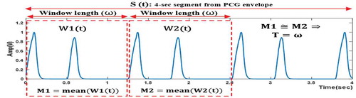
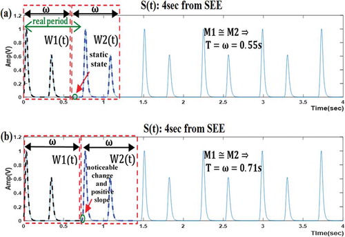
In this stage, a single cardiac cycle is segmented from the preprocessed PCG signal in order to be used for extracting features in the next stage. An automatic segmentation algorithm was proposed that works for the nine PCG signal cases. The goal of this algorithm is to determine the single cardiac cycle length, representing the period (T), by detecting the periodicity within a 4-second segment (S(t)) from the PCG envelope. This 4-second segment is sufficient to contain at least two heart cycles since the heart period range is 0.5–1.5 sec. The key principle for determining T can be summarized as follows (as seen in Figure 2): Two adjacent windows (W1(t) and W2(t)) with the same length (ω) are defined within S(t). ω is gradually increased by a fixed step (20msec), spanning the range of 0.5–1.5 sec. After every increase, the mean values (M1 and M2) of the two adjacent windows are calculated and the (M1≅ M2) condition is examined. If this condition is met, which means the same signal is detected in the two adjacent windows, the period is determined as (T = ω) and the algorithm is stopped.

Figure 2. A visual illustration of the approach used for determining the period (T)

The flow chart of the proposed automatic segmentation algorithm is shown in detail in Figure 3. It consists of three phases.

Figure 3. The flow chart of the proposed automatic segmentations algorithm

2.1.3.1. Phase 1

The goal of this phase is to obtain the envelope of the PCG signal. At first, murmurs are attenuated which helps in obtaining a smoother envelope. Since the frequency range of murmurs is 100–600 Hz (Patidar & Pachori, 2013), the preprocessed PCG signal (PCG(t)) is filtered with a low-pass zero-phase filter with a cut-off frequency of 100 Hz. Next, Shannon Energy Envelope (SEE) given by (1), where x represents the murmur-attenuated signal, is computed using a fixed window of 20msec (Suhas et al., 2017).

(1) $SEE=-x^{2}log\left(x^2\right)$(1)

2.1.3.2. Phase 2

The purpose of this phase is to extract a 4-sec segment (S(t)) from the SSE, whereas S(t) must start with a required onset (δ_0), that is determined according to two proposed main criteria:

1. First criterion: The signal must start with a noticeable change in amplitude. This is attained by calculating the standard deviation within 20msec of the beginning of the signal. The first criterion is met when the value of this standard deviation is found to be higher than (ε = 0.01). The value of ε was obtained empirically and works for the nine cases of PCG signal.

2. Second criterion: The signal must start with a positive increase in the rate of change. This is achieved by calculating the slope within 20msec of the beginning of the signal. The second criterion is met when the calculated value of the slope is found to be positive.

First of all, S(t) is defined within the time range of [δ→δ + 4 sec], where δ is a variable that holds an initial value of zero. Next, δ is gradually increased by a fixed step (20msec) until the two previous criteria are met. Thus, the desired onset is defined as (δ_0 = δ).

2.1.3.3. Phase 3

The main objective of this phase is to determine the signal period (T) in order to segment a single cardiac cycle from the PCG signal. In the beginning, a window (W1(t)) is defined within S(t). This window is measured ω in length and spans the time range [δ_0→δ_0 + ω]. After that, the mean value (M1) of W1(t) is calculated. Subsequently, a second window (W2(t)) that is adjacent to W1(t) is defined within S(t). W2(t) is also measured ω in length but spans the time range [δ_0 + ω→δ_0 + 2 ω]. Following that, the mean value (M2) of W2(t) is calculated. W2(t) must also adhere to the two proposed criteria, which means that the standard deviation and the slope are calculated within 20mes of the beginning of W2(t). Then, ω gradually increases by a fixed step (20msec) within a range of 0.5–1.5 sec until the following condition, which consists of two parts, is met: 1) |M1-M2|<(ε_M = 0.015), in other words M1≅ M2, where ε_M is an experimental value, 2) W2(t) meets the requirements of the two main criteria. Finally, T is defined as (T = ω) and the single cardiac cycle (C(t)) is segmented from PCG(t), where the time range of C(t) is [δ_0→δ_0 + T].

2.1.3.4. Discussion

In this subsection, the importance of the two proposed main criteria is discussed, some results of the algorithm are shown then the algorithm’s performance is evaluated.

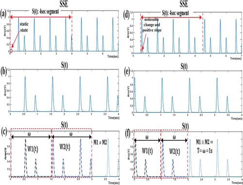
Figure 4 illustrates two cases for extracting the 4-second segment (S(t)) from the SEE. In subfigures (a)-(c), the two main criteria were not considered. At a closer inspection, we notice that the (M1≅ M2) condition was not met and the algorithm was terminated after failing to determine the period (T). The reason for this failure can be traced to the incorrect extraction of S(t), seeing that it was extracted starting from a static state of the SEE. By contrast, subfigures (d)–(f) show a successful algorithm sequence when the two main criteria were considered. S(t) was extracted after detecting both a noticeable change in amplitude and a positive signal slope. The algorithm ended when the (M1≅ M2) condition was met and the value of T was defined as equal to the window length (ω).

Figure 4. Illustrating the importance of satisfying the two main criteria for extracting the 4-sec segment from the SEE. These two criteria are not considered in (a)–(c) but considered in (d)–(f). (a), (d) Shannon Energy Envelope (SEE) of PCG signal; (b), (e) 4-sec segment from the SEE; (c), (f) determining the period (T)

Figure 5 illustrates two cases for defining the second window (W2(t)) within S(t). Subfigure (a) represents the case of incorrect algorithm result, when the two main criteria were ignored. The algorithm finished when the (M1≅ M2) condition was met, even though the resultant value of T (determined to be equal to 0.55 sec) was incorrect. Subfigure (b), however, shows that meeting the requirements of the two main criteria is necessary to obtain correct results. The algorithm finished when the (M1≅ M2) condition was met, which in this case, translates to a value of T that equals ω (0.71 sec).

Figure 5. Illustrating the importance of satisfying the two main criteria for defining the second window (W2(t)) within S(t). (a) determining the period (T), where the two main criteria are ignored; (b) determining the period (T), where the two main criteria are considered

The aforementioned analysis demonstrates the importance of complying with the two main criteria proposed by the authors.

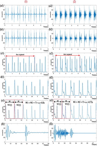
Figure 6 shows segmentation algorithm results for segmenting a single cardiac cycle from the PCG signal for (1) normal case and (2) abnormal case (aortic stenosis).

Figure 6. Segmentation algorithm results for PCG signals for (1) normal case and (2) abnormal case: (a1), (a2) preprocessed PCG signal; (b1), (b2) the murmur-attenuated signal; (c1), (c2) Shannon Energy Envelope (SSE); (d1), (d2) 4 sec segment from the SSE; (e1), (e2) determining the period (T); (f1), (f2) a single-segmented cardiac cycle

The proposed algorithm was tested on the adopted database (200 PCG signals). At First, the cardiac cycles were segmented manually with the help of a physician as a reference. Afterward, accuracy was computed to evaluate the performance of the algorithm as follows:

(2) $Accuracy\left(\mathrm{\%}\right)=\frac{correctlysegmentedcardiaccycles}{totalcardiaccycles}\times 100$(2)

In this research, the correctly segmented cardiac cycles are considered to fit if they are within an acceptance range of ±40 msec. As a result, an accuracy of 96% was obtained.

2.1.4. Feature extraction

First, a large number of features were extracted from the single-segmented cardiac cycle. After that, the importance of those features was defined by using a feature selection algorithm, ReliefF (Kononenko et al., 1997). Then, the highly informative features were chosen by eliminating the features with little predictive information. As a result, 11 features were adopted in this study: one feature in the time domain, three features in the frequency domain, and seven features in the wavelet decomposition domain.

• Time domain feature: It is the standard deviation of the absolute value of the single cycle (std) which is computed according to (3), where N is the total sample number of signal, x_i is the ith sample value, mean abs is the mean of the absolute value of the signal.

  (3) $stdabs={\left(\frac{{\sum }_{i=1}^N{\left(\left|x_i\right|-meanabs\right)}^2}{N-1}\right)}^{\frac{1}{2}}$(3)

• Frequency domain features: Here, the Fast Fourier Transform (FFT) and the Power Spectral Density (PSD) of the single cycle are calculated. Then, three features based on the FFT and PSD are extracted:

  1. Mean frequency: It is computed according to (4), where N is a number of frequency bins in the FFT of one cardiac cycle, f_i and y_i are frequency and intensity (in dB scale) of the FFT of the single cycle at bin i respectively (Emre & Uguz, 2011).

     (4) $meanfrequency=\frac{{\sum }_{i=1}^N{y}_i.f_i}{{\sum }_{i=1}^N{y}_i}$(4)

  2. Spectrum intensity: It is computed according to (5).

     (5) $spectrumintensity=\sum _{i=0}^N\left|y_i\right|$(5)

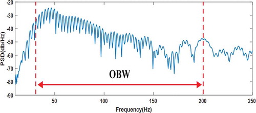
  3. OBW: It is the 99% Occupied bandwidth of the PSD (MathWorks). A Python function was written in order to compute OBW. Figure 7 illustrates the obtained OBW in relation to the PSD curve of the single cycle of normal PCG signal.

     Figure 7. OBW illustrated on PSD curve of the single cycle of normal PCG signal

     

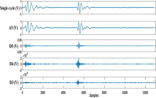
• Wavelet decomposition features: Here, the single cycle is subjected to five levels of Daubechies db6 wavelet decomposition (Meziani et al., 2012). After that, four coefficients (approximation five, detail five, detail four, detail three) are considered (see Figure 8) and seven features based on these coefficients are extracted:

  Figure 8. Wavelet approximation coefficient (A5) and Wavelet detail coefficients (D5, D4, D3) resulting from decomposing the single cycle of normal PCG signal with ‘db6ʹ wavelet

  

  1. Mean of absolute value of detail five coefficients (mean abs (D5)).

  2. Mean of absolute value of detail four coefficients (mean abs (D4)).

  3. Mean of absolute value of detail three coefficients (mean abs (D3)).

  4. Standard deviation of approximation five coefficients (std (A5)).

  5. Standard deviation of detail five coefficients (std (D5)).

  6. Standard deviation of detail four coefficients (std (D4)).

  7. Standard deviation of detail five coefficients (std (D3)).

2.1.5. Classification

Different types of intelligent classification techniques are used in the field of systems engineering and biomedical (Darwish et al., 2018; Souliman et al., 2013). At the present stage, among different varieties of artificial intelligence techniques, artificial neural networks, and their architectures (Joukhadar et al., 2020; Souliman et al., 2014), the feedforward artificial neural network (ANN) with error backpropagation training algorithm was chosen for the classification process (see Figure 9) because it is considered the most widely used model for the purpose of pattern recognition in the biomedical field (Ahmad, 2011; Kumar et al., 2018; Uğuz, 2012). This ANN used here contained three layers: The input layer has 11 points that represent the extracted features. The hidden layer has nine neurons that represent 75% of the 11 input points. And the output layer has four neurons for encoding the nine target cases of PCG signal in binary.

Figure 9. The feedforward backpropagation ANN used in classification

Six models of feedforward backpropagation ANNs, which vary in the activation functions, were experimented with to select the best model that has high accuracy. These models were trained with 140 instances (70% of the dataset) and tested with 60 instances (30% of the dataset). The performance of these models was evaluated through classification accuracy (the ratio of correct predictions to the total predictions). Table 1 shows the performance of these backpropagation ANN models.

Table 1. The performance of several feedforward backpropagation ANN models

Feedforward backpropagation ANN model	Activation function in the hidden layer	Activation function in the output layer	Classification accuracy %
1	Logsig	Tansig	91.66
2	Tansig	Logsig	93.33
3	Logsig	Pureline	90
4	Tansig	Pureline	93.33
5	Logsig	Logsig	95
6	Tansig	Tansig	86.66

It was noticed that the feedforward backpropagation ANN model with logsig activation functions had a high degree of accuracy (95%). Thus, this model was adopted as the best backpropagation ANN.

In addition to the previous backpropagation ANN architecture, other ANN architectures (radial basis ANN, learning vector quantization (LVQ) ANN, and probabilistic ANN) (Aggarwal, 2018; MathWorks, 1111; Mohebali et al., 2020) were experimented with. These ANNs were trained and tested using the same previous dataset. Their structures used here were as following: The radial basis ANN includes nine neurons in the radial basis layer (75% of the 11 input points) and four neurons in the output linear layer to encode the nine target cases in binary. Regarding the LVQ ANN, the competitive layer has 11 neurons (equals the number of input points) and the output linear layer has one neuron for each target case (9 neurons in total). Concerning the probabilistic ANN, the pattern layer contains one neuron for each instance in the training dataset (140 neurons in total) and the competitive layer contains one neuron for each target case (9 neurons). The performance of these architectures was compared to the adopted backpropagation ANN model as shown in Table 2.

Table 2. Performance comparison between the adopted backpropagation

ANN architecture	Classification accuracy %
The adopted backpropagation ANN (with logsig functions) (nine neurons in the hidden layer and four neurons in the output layer)	95
Radial basis ANN (nine neurons in the radial basis layer and four neurons in the output linear layer)	83.33
LVQ ANN (11 neurons in the competitive layer and 9 neurons in the output linear layer)	90
Probabilistic ANN (140 neurons in the pattern layer and 9 neurons in the competitive layer)	95

It was observed that both the backpropagation ANN (with logsig functions) and the probabilistic ANN had the best performance (95%). However, the probabilistic ANN is more complex and requires more memory space to store the model. Thus, the backpropagation ANN (with logsig functions) was realized as the best and simplest classifier with regards to the classification of the nine cases of PCG signal.

2.2. Design and implementation of the diagnostic hardware system

Generally, the hardware of the diagnostic system consists of a PCG signal acquisition module connected to a processing and displaying unit, which is represented by a Raspberry Pi connected to a touch screen, as shown in Figure 10. The Raspberry Pi processes the PCG signal according to the proposed disease classification approach (preprocessing, applying the automatic segmentation algorithm, extracting the 11 features, and applying the best classifier). A demo of a clinical test process using the diagnostic hardware system is shown in Figure 11.

Figure 10. The diagnostic hardware system

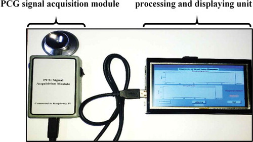
Figure 11. [Courtesy of Medical Electronics Lab], A demo of a clinical test process using the diagnostic hardware system

2.2.1. PCG signal acquisition module

The function of this module is to pick up the PCG signal, condition it, and convert it to a digital format so it can be sent to the Raspberry Pi through the USB port. The block diagram of this module is illustrated in Figure 12.

Figure 12. The block diagram of PCG signal acquisition module

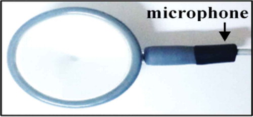
A condenser microphone was used to acquire the PCG signal. This microphone is fixed in a tube with close proximity to the chest piece as shown in Figure 13. The acquired PCG signal is then passed to the conditioning circuit which consists of three sections. First, a high pass filter, with a cut-off frequency of 0.15 Hz, used for removing baseline noise. Second, an amplifier circuit with a gain value of 20. Third, a fourth-order low-pass Butterworth filter, with a cut-off frequency of 800 Hz, which helps in removing high noise components. The resultant conditioned PCG signal is then passed to the USB sound card, which contains a 16-bits analog to digital converter (ADC) with a sample frequency of up to 44.1 kHz. Finally, the digital output is sent to the Raspberry Pi through its USB port.

Figure 13. Connecting the microphone to the chest piece

2.2.2. Processing and displaying unit

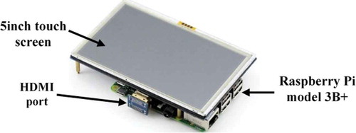
This unit consists of a Raspberry Pi (model 3B+) where the processing of the PCG signal is done, in addition to a 5-inch touch screen for displaying the diagnosis result. This unit is illustrated in Figure 14.

Figure 14. Processing and displaying unit

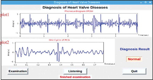
A graphical user interface (GUI) was designed in the software of Raspberry Pi as shown in Figure 15. This GUI displays the diagnosis result after the PCG signal, coming from the acquisition module, is processed according to the proposed disease classification approach. The GUI also makes it possible to listen to the recorded patient heart sounds by pressing the “listen” button. When the “Examination” button is pressed, an order is given to the acquisition module to record a PCG signal for a time period of 5 seconds. The recorded signal is shown in the ‘plot1ʹ window; moreover, the signal is processed to obtain the segmented cardiac cycle and then shown in the ‘plot2ʹ window. Finally, the classification result appears in the “Diagnosis Result” text box.

Figure 15. The system’s GUI designed in the software of Raspberry Pi

3. Results and discussion

The diagnostic hardware system was clinically tested in real time on 50 subjects encompassing the nine valvular heart cases with the help of two cardiologists. Where the performance of the system, as shown in Table 3, was evaluated by calculating three metrics, namely accuracy, sensitivity, and specificity. These metrics are given by (6), (7), and (8), where TP, TN, FP, and FN represent true positives, true negatives, false positives, and false negatives, respectively (Ahmad, 2011; Uğuz, 2012).

(6) $spectrumintensity=\sum _{i=0}^N\left|y_i\right|$(6)

(7) $Sensitivity=\frac{TP}{TP+FN}\times 100$(7)

(8) $Specificity=\frac{TN}{TN+FP}\times 100$(8)

Table 3. Obtained performance metrics of the diagnostic hardware system

Accuracy	Sensitivity	Specificity
96%	95.23%	100%

A comparison of the proposed diagnostic system with state-of-the-art systems is presented in Table 4. For systems that use the PCG signal to diagnose heart valve conditions, the proposed system has three advantages: First, it is capable of diagnosing more heart valve cases. Second, it uses an automatic segmentation method in the time domain which needs less processing time. Third, it is able to examine patients in real time. It must be noted that there is a previous system that is similar to the proposed system, but it relies on Electrocardiogram (ECG) signal to diagnose non-valvular diseases (arrhythmias). However, the proposed system is superior to the ECG system in regard to the number of diagnosed heart conditions.

Table 4. Comparison between the proposed system and previous systems

Reference	Used signal	No. of diagnosed heart conditions	Segmentation method	Diagnosis method
(Grzegorczyk et al., 2016)	PCG	Two valvular heart cases	Based on hidden markov model (needs a long processing time)	Pre-recorded signal analysis
(Emre & Uguz, 2011)	PCG	Three valvular heart cases	Manually	Pre-recorded signal analysis
(Noman et al., 2018)	PCG	Four valvular heart cases	Based on wavelet decomposition (needs a long processing time)	Pre-recorded signal analysis
(Suboh et al., 2008)	PCG	Five valvular heart cases	Manually	Pre-recorded signal analysis
(Alfarhan et al., 2018)	Electrocardiogram (ECG)	Five nonvalvular cases (arrhythmias)	Based on a fixed time window (needs a short processing time)	Real-time patient examination
Proposed system	PCG	Nine valvular heart cases	Using a proposed algorithm in the time domain (needs a short processing time)	Real-time patient examination

4. Conclusion

In this paper, a Raspberry Pi-based system has been proposed for the diagnosis of nine common valvular heart cases (normal one and eight pathological ones) by processing the PCG signal. First, a disease classification approach has been developed. The developed approach consists of five steps, namely obtaining PCG signals, preprocessing, segmentation, feature extraction, and classification. The diagnostic hardware system has been designed and implemented. It consists of a PCG signal acquisition module and a Raspberry Pi connected to a touch screen. The developed classification approach has been implemented, together with a GUI, in the software of the Raspberry Pi to enable it to detect the diseases in real-time. The proposed system has been clinically tested on 50 real subjects covering the nine cases. It has been shown that the accuracy of the system is 96% with a sensitivity factor of 95.23% and a specificity factor of 100%.

The developed system has been proved to be superior to other systems developed in the literature review, especially in relation to the number of diagnosed valve cases. It is also portable, low cost, and provides the diagnosis result immediately, which is useful for rural health-care clinics as a primary diagnosis tool. Future improvements to the system will focus on enlarging the optimal classifier database, in addition to testing a large number of valve patients. With the aim of adopting this system as an official diagnostic device in the medical community.

Additional information

Funding

The authors received no direct funding for this research.

Notes on contributors

Abdulkader Joukhadar

Abdulkader Joukhadar is a Professor of Intelligent Control Systems at the Dept. Mechatronics Engineering, Faculty of Electrical and Electronic Engineering, University of Aleppo, Syria. He received his Ph.D. degree from Aberdeen University, UK in 2004. His research interests include Robot Control, Probabilistic Robotics, and Intelligent Control Systems. Louay Chachati received the Ph.D. degree from the Bioengineering Unit, University of Strathclyde, U.K, in 1991. His main areas of interest are Electronics, Medical Assistance Systems and biomedical instrumentation.

Mohammed Al-Mohammed

Mohammed Al- Mohammed received his Ph.D. from the INPT, France in 2003. His research interests include Electronics, PCB technology, and Artificial Intelligence.

Obada Albasha

Obada Albasha is a Ph.D. candidate at the Department of Electronic Engineering, faculty of Electrical and Electronic Engineering, University of Aleppo. His main areas of interest are Biomedical Signal Processing, Artificial Intelligence and Embedded Systems.

References

- Aggarwal, C. (2018). Neural networks and deep learning: A textbook (1st ed. 2018 ed.). Springer.
- Ahmad, W. (2011). Heart murmur detection/classification using cochlea-like pre-processing and artificial intelligence. International Journal of Biomedical Engineering and Technology, 7(1), 87–16. https://doi.org/10.1504/IJBET.2011.042500
- Alfarhan, K., Mashor, M., Saad, A., & Omar, M. (2018). Wireless heart abnormality monitoring kit based on Raspberry Pi. Journal of Biomimetics, Biomaterials and Biomedical Engineering, 35, 96–108. https://doi.org/10.4028/www.scientific.net/JBBBE.35.96
- Amirjani, A., Yousefi, M., & Cheshmaroo, M. (2014). Parametrical optimization of stent design; a numerical-based approach. Computational Materials Science, 90, 210–220. https://doi.org/10.1016/j.commatsci.2014.04.002
- Cabrera, M., Sanders, B., Goor, O., Driessen-Mol, A., Oomens, C., & Baaijens, F. (2017). Computationally designed 3D printed self-expandable polymer stents with biodegradation capacity for minimally invasive heart valve implantation: A proof-of-concept study. 3D Printing and Additive Manufacturing, 4(1), 19–29. https://doi.org/10.1089/3dp.2016.0052
- Classifying Heart Sounds Challenge. (2016). Peterjbentley.com. http://www.peterjbentley.com/heartchallenge
- Darwish, A. H., Joukhadar, A., & Kashkash, M. (2018). Using the bees algorithm for wheeled mobile robot path planning in an indoor dynamic environment. Cogent Engineering, 5(1), 1426539.
- Emre, G., & Uguz, H. (2011). Classification of heart sounds based on the least squares support vector machine. International Journal of Innovative Computing, Information & Control, 7(12), 7131–7144.
- Firuzbakht, F., Fallah, A., Rashidi, S., & Khoshnood, E. (2018). Abnormal heart sound diagnosis based on phonocardiogram signal processing. 26th Iranian Conference on Electrical Engineering (pp. 1450–1455). IEEE. https://doi.org/10.1109/ICEE.2018.8472410
- Grzegorczyk, I., Solinski, M., Lepek, M., Perka, A., Rosinski, J., Rymko, J., Stepien, K., & Gieraltowski, J. (2016). PCG classification using a neural network approach. Computing in Cardiology Conference. Vancouver: IEEE. https://doi.org/10.22489/CinC.2016.323-252
- Hofmann, S., Groß, V., & Dominik, A. (2016). Recognition of abnormalities in phonocardiograms for computer-assisted diagnosis of heart failures. Computing in Cardiology Conference. Vancouver: IEEE. https://doi.org/10.22489/CinC.2016.161-187
- I. eGeneralMedical. (2016). Cardiac auscultation of heart murmurs/CD -user license download only. Egeneralmedical.com. [ Online]. http://www.egeneralmedical.com/listohearmur.html
- Joukhadar, A., Hanna, D. K., & Al-Izam, E. A. (2020). UKF-based image filtering and 3D reconstruction. In Machine Vision and Navigation (pp. 267–289). Cham: Springer.
- Kameswari, M., Vera, R., Maurice, E., & Robert, B. (2010). Valvular heart disease: Diagnosis and management. Mayo Clinic Proceedings, 85(5), 483–500. https://doi.org/10.4065/mcp.2009.0706
- Kononenko, I., SImek, E., & Sikonja, M. (1997). Overcoming the myopia of inductive learning algorithms with RELIEFF. http://citeseerx.ist.psu.edu/viewdoc/summary?doi=10.1.1.56.474020
- Kumar, D., Jadeja, R., & Pande, S. (2018). Wavelet bispectrum-based nonlinear features for cardiac murmur identification. Cogent Engineering. https://doi.org/10.1080/23311916.2018.1502906
- MathWorks. Signal processing ToolboxTM user’s guide. R2017a. https://mafiadoc.com/signal-processing-toolbox_59aefbfb1723ddbec5e2c665.html
- MathWorks. Neural network ToolboxTM user’s guide. R2017b. https://www.academia.edu/34938587/Neural_Network_Toolbox_Users_Guide
- Meziani, F., Debbal, S., & Atbi, A. (2012). Analysis of phonocardiogram signals using wavelet transform. Journal of Medical Engineering & Technology, 36(6), 283–302. https://doi.org/10.3109/03091902.2012.684830
- Mohebali, B., Tahmassebi, A., Meyer-Baese, A., & Gandomi, A. (2020). Probabilistic neural networks: A brief overview of theory, implementation, and application. Elsevier. https://doi.org/10.1016/B978-0-12-816514-0.00014-X
- Noman, F., Ghani, U., Saba, T., Rehman, A., & Iqbal, S. (2018). Microscopic abnormality classification of cardiac murmurs using ANFIS and HMM. Microscopy Research and Technique, 81(5), 449–457. https://doi.org/10.1002/jemt.22998
- Patidar, S., & Pachori, R. (2013). Segmentation of cardiac sound signals by removing murmurs usingconstrained tunable-Q wavelet transform. ELSEVIER. Biomedical Signal Processing and Control, 8(6), 559–567. https://doi.org/10.1016/j.bspc.2013.05.004
- Rick, N., Catherine, O., Robert, B., Blase, C., John, E., Robert, G., Patrick, O., Carlos, R., Nikolaos, S., Paul, S., Thoralf, S., & James, T. (2014). 2014 AHA/ACC guideline for the management of patients with valvular heart disease: Executive summary. AHA, Circulation, 129(23), 2440–2492. https://doi.org/10.1161/CIR.0000000000000029
- Safara, F., Doraisamy, S., Azman, A., Jantan, A., & Ranga, S. (2013). Diagnosis of heart valve disorders through trapezoidal features and hybrid classifier. International Journal of Bioscience, Biochemistry and Bioinformatics, 3(6), 262–265. https://doi.org/10.7763/IJBBB.2013.V3.298
- Singh, A., Dutta, M., & Travieso, K. (2017). Analysis of heart sound for automated diagnosis of cardiac disorders. International Conference and Workshop on Bioinspired Intelligence. Funchal, Portugal: IEEE. https://doi.org/10.1109/IWOBI.2017.7985528
- Souliman, A., Joukhadar, A., Alturbeh, H., & Whidborne, J. F. (2013). Real time control of multi-agent mobile robots with intelligent collision avoidance system. In 2013 Science and Information Conference (pp. 93–98). IEEE.
- Souliman, A., Joukhadar, A., Alturbeh, H., & Whidborne, J. F. (2014). Intelligent collision avoidance for multi agent mobile robots. In Intelligent Systems for Science and Information (pp. 297–315). Cham: Springer.
- Suboh, M., Mashor, M., Saad, A., & Mohamed, M. (2008). Classification of heart valve diseases using correlation analysis. 5th International Conference on Electrical Engineering, Computing Science and Automatic Control (pp. 173–176). IEEE https://doi.org/10.1109/ICEEE.2008.4723402.
- Suhas, K., Hemanth, R., Nayak, S., & Niranjana, B. (2017). A Hybrid Model for Recognizing Cardiac Murmurs From Phonocardiogram Signal. Annual India Conference. IEEE. https://doi.org/10.1109/INDICON.2016.7839002.
- Uğuz, H. (2012). A biomedical system based on artificial neural network and principal component analysis for diagnosis of the heart valve diseases. Journal of Medical Systems, 36(1), 61–72. https://doi.org/10.1007/s10916-010-9446-7
- http://www.3m.com/healthcare/littmann/mmm-library.html
- https://physionet.org/content/challenge-2016/1.0.0
- Zeng, Y., Sun, R., Xianchi, L., Liu, M., Chen, S., & Zhang, P. (2016). Pathophysiology of valvular heart disease (Review). Experimental and Therapeutic Medicine, 11(4), 1184–1188. https://doi.org/10.3892/etm.2016.3048