Optimum conceptual design for the life support systems of manned spacecraft

Abstract

The problem of the optimal design of the life support systems of manned spacecraft is studied in this paper. The aim is to select components of all relevant subsystems to minimize the mass and power consumption and maximize the total technology readiness level while simultaneously satisfying the mission requirements and physical constraints. The model is developed by considering all intercommunication between the subsystems as the optimal assignment. The final problem is a mixed-integer, non-linear programming problem which is solved by a modified evolutionary optimization algorithm. A set of simulations is performed using real data, which demonstrates the efficiency of the proposed method.

Keywords:

• manned space flight
• life support systems
• design optimization
• evolutionary optimization algorithms

PUBLIC INTEREST STATEMENT

In designing a high technology system, there are usually subsystems and components with candidate technologies. Each technology has different specifications and effects on the main system characteristics such as weight, volume, and power consumption. Therefore, selecting appropriate technologies is an essential problem in system design. This paper proposed a systematic way to help the designer in technology selection. The method that simulated the life of whales attempts to find an optimum configuration that satisfies the design requirements. As a case study, the practical problem of spacecraft configuration design is modeled and solved successfully. It leads to a reduction of total weight, power consumption, and improving the technology readiness level.

1. Introduction

The growing demand for space transportation and human-based in-orbit exploration missions has motivated researchers to investigate different designs of modern manned spacecraft. The special characteristics of manned missions, such as extraterrestrial environments, restrictions on the payload of the launch vehicle, the crew’s needs, and safety make the design of manned spacecraft difficult. In the conceptual design phase, where the configuration, subsystems, and technologies have to be determined, designers should make sure of meeting these requirements while controlling the weight, volume, and power. Therefore, the development of methods based on optimization will improve the design procedures and reduce the related costs.

Along with traditional manned spacecraft such as Apollo, Gemini, and Soyuz, there are various examples of optimization approaches for spacecraft design in the literature. For instance, a multi-disciplinary, multi-objective optimization was implemented by Viviani et al. (2017) to design the optimum shape of a re-entry spacecraft. Another example of the outer shape optimization of manned spacecraft was discussed by Ghaedamini Harouni & Mehne (2019), where the shape of the Orion type space capsule was optimized by considering the volumetric efficiency, stability, and aerodynamic heating.

A second class of problems arises from looking for the best layout design. In these types of problems, the subsystems and their related components are given and the question is how to best place them in the spacecraft. As an example, Cuco et al. (2015) presented a multi-objective method for the three-dimensional layout of a spacecraft, which combined a computer-aided design and an optimization tool to find the optimum positions of the equipment in consideration of their mass, inertia, and thermal requirements. Another work on this topic was reported by Hengeveld et al. (2011), where the optimal placement of equipment on satellite panels with the aim of desired heat flux distribution was investigated. A genetic algorithm was implemented to solve the underlying optimization problem.

A third class of problems attempts to either find the best components of the subsystems among many different available options or determine the best design parameters of the components. This approach needs a comparison mechanism for evaluating and comparing trade-offs. Moreover, in these problems, it is necessary to consider the impact of each component or technology on the other subsystems and the mission’s requirements. As an example, the optimization of the power module in a life support system with the minimal total mass of the system was reported by Bartsev (1997).

In the present work, optimization of a life support system (LSS) is under consideration. The aim is to select the best technologies, the relative design, and the operational parameters of the LSS from a database. Therefore, the problem belongs to the third above-mentioned category. The cost criteria include the total weight, power consumption, and the technology readiness level (TRL). There are also constraints on the total volume and biological conditions related to the onboard crew. The procedure includes constructing a database of technologies and the relationships between the components, generating a mathematical model to describe the problem, and developing a tool to solve the resulting optimization problem. The proposed method is evaluated by implementing it on a test case. The mathematical model for describing the problem is an assignment model with scaling weights; therefore, in addition to having binary variables of the assignment problem, there are some variables with floating-point values. To overcome the complexity of such an optimization problem, an evolutionary method that is a modification of the whale optimization algorithm (WOA) is developed. The results of implementing the proposed method on a test case with real data are used to check the validity of the method in practice. The results are also compared with some of the other meta-heuristics.

The rest of the paper is organized as follows. A review on LSSs, components, and related technologies is given in Section 2, and the problem is described. In Section 3, a mathematical model for the problem is determined. The optimization algorithm is then proposed in Section 4. Section 5 presents an analysis of the simulation results. Finally, some concluding remarks are expressed in Section 6.

2. Life support system

In manned space terminology, an LSS refers to a section of the spacecraft that is designed for humans to live and operate. Besides propulsion and reentry, life support is one of the most important challenges in space missions. Therefore, it has been the topic of different published reports and papers. For example, the design analysis of an LSS for the human exploration of Mars was reported by Czupalla et al. (2004). The importance of cost optimization in the development of LSSs was emphasized by Jones & Anderson (2017). A feasibility analysis of an LSS for an interplanetary transport ship was given by Schreck (2017), where an iterative multi-criteria system analysis that had safety, reliability, and TRL considerations were performed. In a recent work, Mehne (2017) identified and controlled an oxygen provider for an LSS.

In the present work, as mentioned in the introduction, an optimization approach is presented to select the relevant technologies when designing the LSS. Therefore, we need to describe the LSS and its components and technologies in this step.

The LSS has to provide a suitable atmosphere with controlled temperature, pressure, and air combination. Moreover, the LSS should manage the food, water, and waste within the capsule during long-term missions.

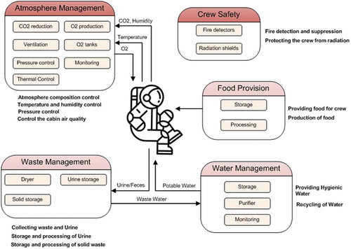
Figure 1. LSS schematic

As schematically depicted in Figure 1, in the general case of a long-term mission, the spacecraft consists of five subsystems, including atmosphere management, crew safety, food provision, waste management, and water management. The expected tasks of each subsystem are written near its block, and the components of each subsystem are indicated by small embedded rectangles. Moreover, interfaces between the subsystems and the crew, and connections among the blocks, are shown by arrows.

The main subsystem at the top of the picture is atmospheric management, which is responsible for the quality of the cabin air, as well as its pressure and temperature. It consists of oxygen tanks, CO${ }_2$ removers, and oxygen generators to provide the required air for the crew’s respiration needs. The heat will increase inside the cabin due to the electrical devices and crew operations. As such, the atmospheric management has to control the temperature by removing the heat from the capsule. Additionally, the pressure can also change, and it is maintained in a prescribed region by the pressure control module. These mentioned tasks will be fulfilled by the atmospheric management subsystem.

To protect the crew from space radiation, specific shielding should be used. This is integrated into the crew’s safety system, which also contains a fire protection module. The crew’s safety and atmospheric management are essential subsystems in a manned spacecraft. The other three blocks can be customized or simplified in short-term and suborbital missions. They manage the water and food for the crew and collect the metabolic and operational waste in the capsule.

2.1. Components and technologies

Each subsystem in the LSS consists of components that perform specific tasks. To design the necessary components there are many choices for the preferred technology, which differ from each other based on performance (power consumption, rates of input and outputs, mass, and volume), cost of supplies, reliability, and TRL. Let us consider, for example, the atmospheric management subsystem, which should continuously manage the levels of CO${ }_2$/O${ }_2$ by generating O${ }_2$ and reducing/removing CO${ }_2$ and other harmful gases. For O${ }_2$ provision components, there are several technologies with successful records, such as:

• In-situ O${ }_2$ tanks,

• Static feed water electrolysis (Fortunato et al., 1988; Powell et al., 1974; Sakurai et al., 2015),

• Water vapor electrolysis (Heppner et al., 1988),

• Oxygen candles (Markowitz et al., 1964; Wang et al., 2018),

• CO${ }_2$ electrolysis (Mehne, 2017),

• Plants.

Each of these technologies has a specific power consumption, oxygen generation rate, weight, volume, and TRL. For example, Table 1 shows the technical and physical specification of the static feed water electrolysis technology.

Table 1. Specification of some of the oxygen generator modules

Parameter	SFWE	WVE	GBR
Mass (kg)	25.06	45.0	9.0
Volume (m${ }^3$)	0.009	0.11	0.002
Power (W)	243	600	15
Pressure
Increment (kPa/d)	79.99		112
Temperature
Increment (K/d)	0.0	0.0	108
O${ }_2$ output (kg/d)	0.907	2.51	0.0004
Local TRL	6	4	8

As indicated in Table 1, every technology has specific mass, volume, power, and other impacts on the total system. These different specifications of the technologies motivated us to arrange for their optimal selection. For example, we may be interested in selecting a technology for the oxygen provider module that has the minimum possible weight and power consumption while being able to produce the required oxygen and satisfying in some predefined volume margin budget. One possible way to face this problem is by sorting all situations and evaluate the trade-offs. However, systematically, we need a tool to solve the problem when there are many possibilities. The mathematical model for this problem is given in the next section.

3. Mathematical modelling

In this section, the problem of the optimal selection of technologies in designing the space capsule is formulated as a mathematical programming problem. In general, such modelling consists of determining the decision, objective functions, and constraints. These components will be explained in the following subsections.

3.1. Decision variables

The decision, or design variables, are unknowns that specify the design parameters directly or indirectly. In the present case where the selection of technologies for the subsystem components is desired, the variables are binary. They should indicate whether a specific technology for a component has been selected in the optimal configuration or not. Therefore, we consider the following definition for the decision variable:

(1) $x_{ijk}=\left\{\begin{array}{cc}1& \mathrm{i}\mathrm{f}\mathrm{t}\mathrm{h}\mathrm{e}\mathrm{t}\mathrm{e}\mathrm{c}\mathrm{h}\mathrm{n}\mathrm{o}\mathrm{l}\mathrm{o}\mathrm{g}\mathrm{y}k\mathrm{i}\mathrm{s}\mathrm{s}\mathrm{e}\mathrm{l}\mathrm{e}\mathrm{c}\mathrm{t}\mathrm{e}\mathrm{d}\mathrm{f}\mathrm{o}\mathrm{r}\mathrm{c}\mathrm{o}\mathrm{m}\mathrm{p}\mathrm{o}\mathrm{n}\mathrm{e}\mathrm{n}\mathrm{t}j\mathrm{o}\mathrm{f}\mathrm{s}\mathrm{u}\mathrm{b}\mathrm{s}\mathrm{y}\mathrm{s}\mathrm{t}\mathrm{e}\mathrm{m}i\\ 0& \mathrm{o}\mathrm{t}\mathrm{h}\mathrm{e}\mathrm{r}\mathrm{w}\mathrm{i}\mathrm{s}\mathrm{e}\end{array}\right.$(1)

where $i=1,2,\cdots ,N_{sub}$ is the index of the subsystem in the capsule, $j=1,2,\cdots ,N_{comp}(i)$ is the index of the components in the subsystems, and $k=1,2,\cdots ,N_{tech}(i,j)$ is the index for technologies. Here, $N_{sub}$ is the number of spacecraft subsystems, $N_{comp}(i)$ is the number of components in the $j$-th subsystem, and $N_{tech}(i,j)$ indicates the number of available technologies for the $j$-th component of the $i$-th subsystem.

If, for example, the solution $x_{123}=1$ means that the third technology is used for the second component of the first subsystem.

Moreover, we need a scaling factor for each technology to balance the specification information and the requirements. Here $s_{ijk}$ is the scaling factor or weight of technology $k$ for component $j$ in the $i$-th subsystem. For example, if $s_{432}=2.5$, then the second technology for the third component of the fourth subsystem will be used with a scaling factor of 2.5. Then, the weight, power, rate, and the other specifications will be multiplied by 2.5 in the model and subsequent computations. Trivially, $x_{ijk}=0$ is equivalent to $s_{ijk}=0$ and vice versa. On the other hand, $x_{ijk}=1$ implies that $s_{ijk}>0$ and vice versa.

3.2. Objective functions

Let us now consider three objective functions for the underlying problem: weight, power consumption, and TRL. The aim is to minimize the total weight and electrical power and to maximize the TRL. Here $w_{ijk}$, $p_{ijk}$, and $t_{ijk}$ are, respectively, the weight, power consumption, and TRL of technology $k$ of component $j$ in the $i$-th subsystem. Then, the objective functions are defined as follows:

(2) $J_1=\sum _{i=1}^{N_{sub}}\sum _{j=1}^{N_{comp}(i)}\sum _{k=1}^{N_{tech}(i,j)}{s}_{ijk}{w}_{ijk}{x}_{ijk}(\mathrm{W}\mathrm{e}\mathrm{i}\mathrm{g}\mathrm{h}\mathrm{t})$(2)

(3) $J_2=\sum _{i=1}^{N_{sub}}\sum _{j=1}^{N_{comp}(i)}\sum _{k=1}^{N_{tech}(i,j)}{s}_{ijk}{p}_{ijk}{x}_{ijk}(\mathrm{P}\mathrm{o}\mathrm{w}\mathrm{e}\mathrm{r})$(3)

(4) $J_3=\sum _{i=1}^{N_{sub}}\sum _{j=1}^{N_{comp}(i)}\sum _{k=1}^{N_{tech}(i,j)}{t}_{ijk}{x}_{ijk}(\mathrm{T}\mathrm{R}\mathrm{L})$(4)

The above objective function may be combined into a single one as

(5) $\frac{\frac{0.5J_1}{Ma{x}_W}+\frac{0.5J_2}{Ma{x}_P}}{1+\frac{J_3}{9}}$(5)

where $Ma{x}_W$ and $Ma{x}_P$ are the predefined maximum weigh and power and TLR$\le 9$. Since $J_1$, $J_2$ and $J_3$ have a different range of values, scaling them as given in ((5)) will prevent to overcome one of them to the others.

3.3. Constraints

In this subsection, we specify the constraints of the problem. The first constraint is to ensure that at least one technology is assigned to each component. This defines a group of constraints as follows:

(6) $\sum _{k=1}^{N_{tech}(i,j)}{x}_{ijk}\ge 1,i=1,2,\cdots ,N_{sub},j=1,2,\cdots ,N_{comp}(i)$(6)

The second constraint is related to the volumetric budget:

(7) $\sum _{j=1}^{N_{comp}(i)}\sum _{k=1}^{N_{tech}(i,j)}{s}_{ijk}{v}_{ijk}{x}_{ijk}\le V_i,i=1,2,\cdots ,N_{sub}$(7)

where $V_i$ denotes the volume budget of the $i$-th subsystem and $v_{ijk}$ is the volume occupied by the $k$-th technology of the $j$-th component of the $i$-th subsystem.

The essential constraints are restrictions related to human health. The oxygen generation rate should be between 0.636 and 1 kg per day per crew member based on standards, and CO${ }_2$ removal has to be greater than 1 kg per day per crew member. The internal temperature should be between 18.3 and 26.7°C, the humidity ratio should be between 25% and 70%, and the cabin pressure should be between 99.9 kPa and 102.7 kPa. These constraints were implemented, respectively, as follows:

(8) $0.635\le \sum _{k=1}^{N_{tech}(1,j)}{s}_{1jk}rO{2}_{1jk}{x}_{1jk}\le 1$(8)

(9) $1\ast N_{crew}\le \sum _{k=1}^{N_{tech}(1,j)}{s}_{1jk}rCO{2}_{1jk}{x}_{1jk}$(9)

(10) $-4.2\le \sum _{i=1}^{N_{sub}}\sum _{j=1}^{N_{comp}(i)}\sum _{k=1}^{N_{tech}(i,j)}{s}_{1jk}\delta t_{1jk}{x}_{1jk}\le 4.2$(10)

(11) $-20\le \sum _{j=1}^{N_{comp}(1)}\sum _{k=1}^{N_{tech}(1,j)}{s}_{1jk}\delta h_{1jk}{x}_{1jk}\le 20$(11)

(12) $-1.4\le \sum _{j=1}^{N_{comp}(1)}\sum _{k=1}^{N_{tech}(1,j)}{s}_{1jk}\delta p_{1jk}{x}_{1jk}\le 1.4$(12)

where $rO{2}_{1jk}$, $rCO{2}_{1jk}$, $\delta h_{1jk}$, and $\delta p_{1jk}$ are, respectively, the rate of oxygen generation, the rate of CO${ }_2$ removal, the humidity effect, and the pressure effect of the $k$-th technology on the $j$-th component of the atmospheric management system. The effect of the $k$-th technology on the $j$-th component of the $i$-th system is represented by $\delta t_{1jk}$. Here, $N_{crew}$ shows the number of crew members.

The restrictions and limitations of the other subsystems are modeled similarly. The resulting model is a mixed-integer non-linear programming problem with a single-combined objective function or with three objectives, $J_1$, $J_2$ and $J_3$. In the next section, an effective heuristic algorithm for solving the problem is proposed.

4. The method of optimization

The problem of minimizing Equation (5)(5) $\frac{\frac{0.5J_1}{Ma{x}_W}+\frac{0.5J_2}{Ma{x}_P}}{1+\frac{J_3}{9}}$(5) under constraints 6–12 is a mixed-integer non-linear programming problem. Due to the complexity of this problem, solving it with traditional methods of optimization is time-consuming. In such cases, usually, meta-heuristic methods are popular for solving the problem in a reasonable amount of time. Among several meta-heuristic algorithms, WOA is a recently new nature-inspired optimizer with a successful record for solving optimization methods. Based on the reports given by Abd El Aziz et al. (2017); Aljarah et al. (2018); Mafarja & Mirjalili (2018); Mirjalili & Lewis (2016), WOA has better performance in accuracy and convergent in comparison with other meta-heuristics such as genetic algorithm, particle swarm optimization, ant colony optimization (ACO), population-based incremental learning algorithm, differential evolution, moth-flame optimization (MFO), ant lion optimizer.

Based on the above-mentioned superiority, ease of implementation, independence of derivative, and the ability to find global optimums, in the present research, a modified version of the WOA is utilized to solve the underlying optimization problem.

The original version of this algorithm which is proposed by (Mirjalili & Lewis, 2016) solves single objective, unconstrained problems. It is a stochastic population-based algorithm that simulates the hunting behaviour of whales. The method starts with a set of whales or search agents searching the predefined space for the best solution. Each whale possesses a solution candidate that is updated attractively based on a combination of the best solution and stochastic directions. The process has two main phase of exploration and exploitation. In the exploration phase, a whale examines different directions around for a better solution randomly. This phase helps to avoid trapping at local optima. In the exploitation phase, one of the two methods of shrinking encircling and spiral path search is applied randomly to find better solutions.

For the case of this research, we had to modify it to cover constraint problems with binary and real variables. To handle our constraints, we used an avoidance mechanism that recognized and rejected infeasible solutions. For converting the real decision values of variables a V-shape function was used. The algorithm of the proposed method is as follows:

(i) Setting up: First choose the number of iterations and the number of whales, i.e. $l_b$ and $u_b$, respectively.

(ii) Initialization: Consider a set of $N$ whales or search engines. Each whale keeps an individual solution $(\mathbf{x},\mathbf{s})$ where $\mathbf{x}$ is a three-dimensional vector of binary decision variables defined in Equation (1)(1) $x_{ijk}=\left\{\begin{array}{cc}1& \mathrm{i}\mathrm{f}\mathrm{t}\mathrm{h}\mathrm{e}\mathrm{t}\mathrm{e}\mathrm{c}\mathrm{h}\mathrm{n}\mathrm{o}\mathrm{l}\mathrm{o}\mathrm{g}\mathrm{y}k\mathrm{i}\mathrm{s}\mathrm{s}\mathrm{e}\mathrm{l}\mathrm{e}\mathrm{c}\mathrm{t}\mathrm{e}\mathrm{d}\mathrm{f}\mathrm{o}\mathrm{r}\mathrm{c}\mathrm{o}\mathrm{m}\mathrm{p}\mathrm{o}\mathrm{n}\mathrm{e}\mathrm{n}\mathrm{t}j\mathrm{o}\mathrm{f}\mathrm{s}\mathrm{u}\mathrm{b}\mathrm{s}\mathrm{y}\mathrm{s}\mathrm{t}\mathrm{e}\mathrm{m}i\\ 0& \mathrm{o}\mathrm{t}\mathrm{h}\mathrm{e}\mathrm{r}\mathrm{w}\mathrm{i}\mathrm{s}\mathrm{e}\end{array}\right.$(1) and $s$ is a three-dimensional vector of real-valued scales. The initial population is generated randomly. The values of the components of $x$ are chosen randomly between $[0,1]$, then a sigmoid transform is used to map them to $0,1$. For example, if ${\hat{x}}_{ijk}$ is the initial value between 0 and 1, the new binary value is selected based on a random number $p$ and the following relation:

(13) $x_{ijk}=\left\{\begin{array}{cc}0& \mathrm{i}\mathrm{f}p<\frac{1}{1+exp(-{\hat{x}}_{ijk})}\\ 1& \mathrm{o}\mathrm{t}\mathrm{h}\mathrm{e}\mathrm{r}\mathrm{w}\mathrm{i}\mathrm{s}\mathrm{e}\end{array}\right.$(13)

The values of the $s$ components are also chosen randomly in a predefined range $[l_b,u_b]$. Then, the resulting pair is check for feasibility, that is, whether they satisfy constraints 6–12. If the solution is not feasible, then the process of random solution generation is repeated. At the end of the initialization step, the following set of feasible solutions is available:

(14) $\{({\mathbf{x}}_1,{\mathbf{s}}_1),({\mathbf{x}}_2,{\mathbf{s}}_2),\cdots ,({\mathbf{x}}_N,{\mathbf{s}}_N)\}$(14)

(iii) Evaluation: In this next phase, the quality of the solutions is evaluated by calculating $J_1$, $J_2$, $J_3$ and the combined performance index of each whale. Then, the best solution (i.e. the whale with the minimum objective function) is determined and marked as $({\mathbf{x}}^{\ast },{\mathbf{s}}^{\ast })$.

(iv) Update: In this step, the values of the solutions are updated using the lead whale’s information. This updating step is performed in three ways based on the value of a random number $p\in [0,1]$ as follows:

(15) ${\stackrel{\mathbf{ˆ}}{\mathbf{x}}}_i^{new}=\left\{\begin{array}{c}{\mathbf{x}}^{\ast }-A\left|C{\mathbf{x}}^{\ast }-{\mathbf{x}}_i\right|,\mathrm{i}\mathrm{f}p<0.5,\hspace{0.17em}\left|A\right|\le 1\\ {\mathbf{x}}^{\ast }+\left|{\mathbf{x}}^{\ast }-{\mathbf{x}}_i\right|e^{bl}.cos(2\pi l),\mathrm{i}\mathrm{f}p\ge 0.5,\hspace{0.17em}\left|A\right|\le 1\\ {\mathbf{x}}_{rand}-A\left|C{\mathbf{x}}_{rand}-{\mathbf{x}}_i\right|\mathrm{i}\mathrm{f}p⟨0.5,\hspace{0.17em}\left|A\right|⟩1\end{array}\right.$(15)

where:

$A=2.a.r-r\mathrm{a}\mathrm{c}\mathrm{o}\mathrm{e}\mathrm{f}\mathrm{f}\mathrm{i}\mathrm{c}\mathrm{i}\mathrm{e}\mathrm{n}\mathrm{t}\mathrm{v}\mathrm{e}\mathrm{c}\mathrm{t}\mathrm{o}\mathrm{r}$

$C=2.r\mathrm{a}\mathrm{c}\mathrm{o}\mathrm{e}\mathrm{f}\mathrm{f}\mathrm{i}\mathrm{c}\mathrm{i}\mathrm{e}\mathrm{n}\mathrm{t}\mathrm{v}\mathrm{e}\mathrm{c}\mathrm{t}\mathrm{o}\mathrm{r}$

$\begin{array}{rl}& a=\mathrm{a}\mathrm{v}\mathrm{e}\mathrm{c}\mathrm{t}\mathrm{o}\mathrm{r}\mathrm{o}\mathrm{f}\mathrm{c}\mathrm{o}\mathrm{n}\mathrm{s}\mathrm{t}\mathrm{a}\mathrm{n}\mathrm{t}\mathrm{s}\mathrm{l}\mathrm{i}\mathrm{n}\mathrm{e}\mathrm{a}\mathrm{r}\mathrm{l}\mathrm{y}\mathrm{d}\mathrm{e}\mathrm{c}\mathrm{r}\mathrm{e}\mathrm{a}\mathrm{s}\mathrm{e}\mathrm{d}\mathrm{f}\mathrm{r}\mathrm{o}\mathrm{m}2\mathrm{t}\mathrm{o}0\mathrm{d}\mathrm{u}\mathrm{r}\mathrm{i}\mathrm{n}\mathrm{g}\mathrm{i}\mathrm{t}\mathrm{e}\mathrm{r}\mathrm{a}\mathrm{t}\mathrm{i}\mathrm{o}\mathrm{n}\mathrm{s}\\ & \mathrm{w}\mathrm{i}\mathrm{t}\mathrm{h}i-\mathrm{t}\mathrm{h}\mathrm{c}\mathrm{o}\mathrm{m}\mathrm{p}\mathrm{o}\mathrm{n}\mathrm{e}\mathrm{n}\mathrm{t}\mathrm{d}\mathrm{e}\mathrm{f}\mathrm{i}\mathrm{n}\mathrm{e}\mathrm{d}\mathrm{a}\mathrm{s}{a}_{\mathrm{i}}=2-i\frac{2}{MaxIter}.i\mathrm{i}\mathrm{s}\mathrm{t}\mathrm{h}\mathrm{e}\mathrm{i}\mathrm{t}\mathrm{e}\mathrm{r}\mathrm{a}\mathrm{t}\mathrm{i}\mathrm{o}\mathrm{n}\\ & \mathrm{c}\mathrm{o}\mathrm{u}\mathrm{n}\mathrm{t}\mathrm{e}\mathrm{r}\mathrm{a}\mathrm{n}\mathrm{d}\mathrm{M}\mathrm{a}\mathrm{x}\mathrm{I}\mathrm{t}\mathrm{e}\mathrm{r}\mathrm{i}\mathrm{s}\mathrm{t}\mathrm{h}\mathrm{e}\mathrm{m}\mathrm{a}\mathrm{x}\mathrm{i}\mathrm{m}\mathrm{u}\mathrm{m}\mathrm{n}\mathrm{u}\mathrm{m}\mathrm{b}\mathrm{e}\mathrm{r}\mathrm{o}\mathrm{f}\mathrm{i}\mathrm{t}\mathrm{e}\mathrm{r}\mathrm{a}\mathrm{t}\mathrm{i}\mathrm{o}\mathrm{n}\mathrm{s}\end{array}$

$b=\mathrm{a}\mathrm{c}\mathrm{o}\mathrm{n}\mathrm{s}\mathrm{t}\mathrm{a}\mathrm{n}\mathrm{t}\mathrm{d}\mathrm{e}\mathrm{f}\mathrm{i}\mathrm{n}\mathrm{i}\mathrm{n}\mathrm{g}\mathrm{t}\mathrm{h}\mathrm{e}\mathrm{s}\mathrm{h}\mathrm{a}\mathrm{p}\mathrm{e}\mathrm{o}\mathrm{f}\mathrm{l}\mathrm{o}\mathrm{g}\mathrm{a}\mathrm{r}\mathrm{i}\mathrm{t}\mathrm{h}\mathrm{m}\mathrm{i}\mathrm{c}\mathrm{s}\mathrm{p}\mathrm{i}\mathrm{r}\mathrm{a}\mathrm{l}$

$l=\mathrm{a}\mathrm{r}\mathrm{a}\mathrm{n}\mathrm{d}\mathrm{o}\mathrm{m}\mathrm{n}\mathrm{u}\mathrm{m}\mathrm{b}\mathrm{e}\mathrm{r}\mathrm{i}\mathrm{n}[-1,1]$

${\mathbf{x}}_{rand}=\mathrm{a}\mathrm{r}\mathrm{a}\mathrm{n}\mathrm{d}\mathrm{o}\mathrm{m}\mathrm{l}\mathrm{y}\mathrm{c}\mathrm{h}\mathrm{o}\mathrm{s}\mathrm{e}\mathrm{n}\mathrm{s}\mathrm{o}\mathrm{l}\mathrm{u}\mathrm{t}\mathrm{i}\mathrm{o}\mathrm{n}\mathrm{a}\mathrm{m}\mathrm{o}\mathrm{n}\mathrm{g}\mathrm{c}\mathrm{u}\mathrm{r}\mathrm{r}\mathrm{e}\mathrm{n}\mathrm{t}\mathrm{p}\mathrm{o}\mathrm{p}\mathrm{u}\mathrm{l}\mathrm{a}\mathrm{t}\mathrm{i}\mathrm{o}\mathrm{n}$

Since the resulting solution ${\stackrel{\mathbf{ˆ}}{\mathbf{x}}}_i^{new}$ may not be binary, a V-shaped transformation (Mirjalili & Lewis, 2013) is used to convert it to binary as follows:

(16) $x_{ijk}^{new}=\left\{\begin{array}{cc}0& \mathrm{i}\mathrm{f}p<\left|\frac{2}{\pi }arctan(\frac{\pi }{2}({\hat{x}}_{ijk}-{\hat{x}}_{ijk}))\right|\\ \hspace{0.17em}& \hspace{0.17em}\\ 1& \mathrm{o}\mathrm{t}\mathrm{h}\mathrm{e}\mathrm{r}\mathrm{w}\mathrm{i}\mathrm{s}\mathrm{e}\end{array}\right.$(16)

In a similar way, and in the same loop with the above-defined parameters, the values of the other parts of the solution, i.e. $s_i$, are updated as indicated below:

(17) ${\mathbf{s}}_i^{new}=\{\begin{array}{c}{\mathbf{s}}^{\ast }-A\left|C{\mathbf{s}}^{\ast }-{\mathbf{s}}_i\right|,\mathrm{i}\mathrm{f}p<0.5,\hspace{0.17em}\left|A\right|\le 1\\ \hspace{0.17em}\\ {\mathbf{s}}^{\ast }+\left|{\mathbf{s}}^{\ast }-{\mathbf{s}}_i\right|e^{bl}.cos(2\pi l),\mathrm{i}\mathrm{f}p\ge 0.5,\hspace{0.17em}\left|A\right|\le 1\\ \hspace{0.17em}\\ {\mathbf{s}}_{rand}-A\left|C{\mathbf{s}}_{rand}-{\mathbf{s}}_i\right|\mathrm{i}\mathrm{f}p⟨0.5,\hspace{0.17em}\left|A\right|⟩1\end{array}$(17)

Here, ${\mathbf{s}}_{rand}$ is a randomly chosen solution among the current population.

After updating, all of the solutions are examined for feasibility. One of the previously examined strategies when facing infeasible solution was to throw away the infeasible solutions and switch to the current solution (Mehne & Mirjalili, 2019). However, in the present work, we repeat the updating procedure until all the solutions become feasible. This approach provides more solutions and a bigger search space.

To implement the method on a special case, we assume that the relating constraints are consistent that is the domain of feasible solutions is not empty, and there exists a global optimum. Another hypothesis that accelerates the convergence is the objective function does not have high local fluctuations.

5. Simulation and results

In this section, the proposed algorithm is examined using data from actual manned spacecraft capsules. The assumptions for this simulation are listed in Table 2.

Figure 2. The objective function in terms of number of iterations

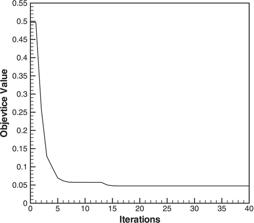
Figure 3. The optimal power, mass, and TRL during each iteration

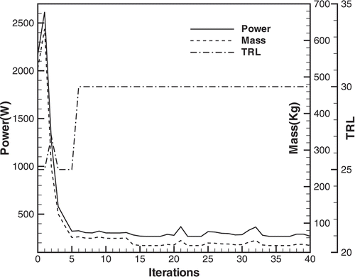
Table 2. Assumptions in the simulation

Capsule mass (kg)	2200
Capsule Volume ($m^3$)	1090
Number of crew	1
Flight type	Orbital
Component operation mode	Continuous

Two subsystems are considered in the simulation: atmosphere management, and water management. The components and technologies of these subsystems are also given in Table 3. The required data and specifications were taken both from (Eckart, 1996; Heppner et al., 1988; Knox et al., 2004; Woods et al., 1975) and by using simple theoretical relations.

Table 3. Matrix of technologies considered in the simulation

Subsystem	Components	Technologies
Atmosphere management	O${ }_2$ provision	SFWE, WVE, GBR
	CO${ }_2$ removal	2-BMS, 4-BMS, ZHG/EDC, SAWD, Bosch-R, Sabatier
Water management	Urine recovery	VCD, VAPCAR, TIMES

The method parameters in the simulation were as follows:

• $b=1$

• Maximum number of iteration = 50

• Number of whales = 30

The source code of the proposed algorithm was written in C++. We executed the program and found the optimal selection of the technologies and scales. To ensure a solution, the program was run 20 times. We used g++ compiler version 7.3.0 on a Linux computer with a 3.3 GHz processor, and the wall clock time of a single execution was 31 milliseconds. Figure 2 presents the corresponding best objective function values obtained during a typical run. The initial objective value was 0.4970, which reduced within 15 iterations to 0.0475. This means a 90.4% reduction and demonstrates a high rate of convergence. The best power, mass, and overall TRL during the iterations are depicted in Figure 3. As indicated, the power started from 2166.8 W and reduced to 267.5 W, which implies a 87.6% reduction in the required electrical power. The mass of components reduced from 523.1 kg to 38.6 kg, that is, the optimal solution resulted in a 92.6% saving in mass. The TRL curve, on the other hand, increased from 25 to 30 in the final design. For this solution, the selected technologies and scaling factors were: (WVE, 0.28), (4-BED, 0.15), (VDC, 0.014), and (VAPCAR, 0.16).

The results of all 20 runs are given in Table 4, where the first and the fourth columns show the run numbers, followed by the corresponding fitness and scales. The third and sixth columns indicate the corresponding scaling factors of selected technology in the optimal solution. For example, in the first row, $s_{112}=0.34$ means that $x_{112}=1$ and the technology 2 is selected for component 1 of the first subsystem with a scaling factor equals to 0.34. Trivially the variables with zero value or zero scales have not been participated in the solution and were not given in the table. The results are in the same order of optimality and the best of them with minimum fitness value equals 0.1005 occurs in the tenth run.

Table 4. The optimal fitness and scales obtained in the simulation

Run no.	Fitness	Scales	Run no.	Fitness	Scales
		$s_{112}=0.34$			$s_{112}=0.25$
1	0.1062	$s_{123}=0.19$	11	0.1178	$s_{122}=0.21$
		$s_{212}=0.95$			$s_{213}=0.90$
		$s_{112}=0.25$			$s_{112}=0.33$
2	0.0775	$s_{124}=0.28$	12	0.1041	$s_{123}=0.17$
		$s_{212}=0.95$			$s_{212}=0.91$
		$s_{112}=0.26$			$s_{112}=0.25$
3	0.1286	$s_{121}=0.55$	13	0.1462	$s_{121}=0.40$
		$s_{211}=0.90$			$s_{213}=0.90$
		$s_{112}=0.34$			$s_{112}=0.74$
4	0.1054	$s_{123}=0.19$	14	0.1932	$s_{123}=0.81$
		$s_{212}=0.90$			$s_{212}=0.90$
		$s_{112}=0.27$			$s_{112}=0.25$
5	0.1100	$s_{124}=0.22$	15	0.1244	$s_{122}=0.32$
		$s_{211}=0.89$			$s_{126}=0.91$
					$s_{211}=0.90$
		$s_{112}=0.26$			$s_{112}=0.26$
6	0.1528	$s_{124}=0.48$	16	0.1073	$s_{122}=0.16$
		$s_{211}=0.90$			$s_{211}=0.90$
		$s_{112}=0.25$			$s_{112}=0.34$
7	0.1302	$s_{124}=0.29$	17	0.1050	$s_{123}=0.19$
		$s_{211}=0.90$			$s_{212}=0.90$
		$s_{112}=0.25$			$s_{112}=0.27$
8	0.1141	$s_{124}=0.24$	18	0.1201	$s_{121}=0.31$
		$s_{213}=0.90$			$s_{126}=0.38$
					$s_{211}=0.91$
		$s_{112}=0.25$			$s_{112}=0.38$
9	0.2128	$s_{124}=0.89$	19	0.1257	$s_{123}=0.29$
		$s_{213}=0.94$			$s_{213}=0.90$
		$s_{112}=0.25$			$s_{112}=0.73$
10	0.1005	$s_{122}=0.15$	20	0.1557	$s_{123}=1$
		$s_{212}=0.91$			$s_{211}=0.49$
					$s_{212}=0.12$
					$s_{213}=0.29$

Since the method is naturally probabilistic, we may find different solutions in different executions. To compare the solutions and frequency of each technology, the value of all obtained variable in the 20 runs are given in Table 5. A column of binary values shows the optimal solution in each individual run. The last two columns of the table show the frequency of the data and the related percentage. Based on these data, the best choice for the oxygen provision component was WVE, which had 100% frequency and 0.25 scaling factor within the solutions, while the other technologies were not advised. For CO${ }_2$ reduction, in most of the cases, two technologies appeared in the solution, where ZHG/EDC with 0.19 scaling factor or SAWD with 0.24 scaling factor was recommended in order to optimally cover the requirements. Finally, for water management, the highest ranked technology was VCD and VAPCAR with approximately 0.90 scaling factor.

Table 5. Results of simulation

Technology	Results	Frequency	Percentage
SFWE	0 0 0 0 0 0 0 0 0 0 0 0 0 0 0 0 0 0 0 0	0	0%
WVE	1 1 1 1 1 1 1 1 1 1 1 1 1 1 1 1 1 1 1 1	20	100%
GBR	0 0 0 0 0 0 0 0 0 0 0 0 0 0 0 0 0 0 0 0	0	0%
2-BMS	0 0 1 0 0 0 0 0 0 0 0 1 0 0 0 0 1 0 0 1	4	20%
4-BMS	0 0 0 0 0 0 0 0 0 1 1 0 0 0 1 1 0 0 0 0	4	20%
ZHG/EDC	1 0 0 1 0 0 0 0 0 0 0 1 0 1 0 0 1 0 1 1	7	35%
SAWD	0 1 0 0 1 1 1 1 1 0 0 0 0 0 0 0 0 0 0 0	6	30%
Bosch-R	0 0 0 0 0 0 0 0 0 0 0 0 0 0 0 0 0 0 0 0	0	0%
Sabatier	0 0 0 0 0 0 0 0 0 0 0 0 0 0 1 0 0 1 0 0	2	10%
VCD	0 0 0 1 0 1 1 1 0 0 0 0 0 0 1 1 0 1 0 1	8	40%
VAPCAR	1 1 0 1 0 0 0 1 0 1 0 1 0 1 0 0 1 0 0 0	8	40%
TIMES	0 0 0 0 0 0 0 1 1 0 1 0 1 0 0 0 0 0 1 1	6	30%

We have also performed a sensitivity analysis on some parameters of the WOA method. The first parameter was the number of iterations. In the analysis, the maximum number of iterations is changed from 10 to 1000 and 20 runs were performed. Then, the corresponding fitness values and wall clock time of executions were gathered. As indicated in Table 6 the variance of fitness has low deviations within 20 runs for each number of iterations and it reduces as the iteration increases. The optimal solutions are also close together that shows the method converges to an optimal solution within a few numbers of iterations. The time of executions is also approximately increasing with iterations as expected. Therefore, the method is fast and converges even for a few numbers of iterations.

Table 6. The effect of changing the maximum number of iterations for 20 runs of algorithm

Iterations	Min. fitness	Variance of fitness	Averaged time (ms)
10	0.0918	$5.4\times {10}^{-2}$	985
20	0.0805	$1.5\times {10}^{-2}$	1017
50	0.0759	$7.9\times {10}^{-3}$	977
100	0.0897	$7.4\times {10}^{-3}$	929
150	0.0922	$3.7\times {10}^{-3}$	990
200	0.0960	$2.3\times {10}^{-3}$	973
500	0.0919	$6.6\times {10}^{-4}$	917
750	0.0853	$6.3\times {10}^{-4}$	1079
1000	0.0873	$2.7\times {10}^{-4}$	1093

As the second parameter, we examine the effect of the whale number. It is expected that by increasing the number of whales that is the number of search agents, the solution is improved. To check the effect of this parameter, it was changed from 10 to 200 and the corresponding results for 20 runs were gathered. The results are given in Table 7, where the first column is the number of whales, the second is the mean of fitness, the third is the best solution within the runs and the last column indicates the averaged wall clock time of execution. As expected the solutions improved by increasing the number of whales. In this case, the best fitness with 10 whales is 0.0987 which is reduced 36% to 0.0630 with 200 whales. Therefore, the method will have accurate results even with a low number of whales, and increasing the number of whales has a low effect on the solution accuracy while increases the complexity of the algorithm linearly. The other parameter of the method is $b$ that indicates the shape of the spirals. To study the effect of this parameter on the best-obtained solutions, a set of runs have been performed with $b$ varying from 0.001 to 5 while the number of iterations and the number of whales kept constant at 100 and 20, respectively. The program executed 20 times for each value and the best result has been recorded. Based on the results which are also given in Figure 4, $b$ does not have a meaningful effect on the result. However, it leads to more stable results near 1.

Figure 4. The effect of $b$ on the best-obtained result.

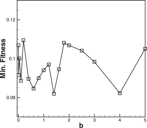
Table 7. The effect of changing the number of whales for 20 runs of algorithm

Whale no.	Aver. fitness	Min. fitness	Averaged time (ms)
10	0.2707	0.0987	564
20	0.1506	0.0957	1075
50	0.1206	0.0700	2517
100	0.1108	0.0756	5105
200	0.1080	0.0630	10,122

Finally, the method was compared with some of the other meta-heuristics. The problem has been solved by genetic algorithm (GA), ACO, and MFO on the same computer. The number of clients and the minimum required fitness of the results were chosen 100 and 0.05 for all methods. The other parameters in implementing these methods are listed below:

• GA: Generation gap = 0.8, crossover rate = 0.95, and mutation rate = 0.05.

• ACO: Information heuristic factor = 3.0, expectation heuristic factor = 3.0, pheromone evaporation factor =0.75, pheromone strength = 50.0.

• MFO: Weight factors = $\frac{1}{3}$.

• WOA: $b=1.0$.

A sensitivity analysis has been also performed with 10% deviation from these values to tune up and finding the best results.

With a fixed order of error, the number of iterations, the number of function evaluations, and the wall clock time were different for methods and show the method performance. The best-obtained results and the related performance parameters have been given and compared in Table 8. Within these algorithms, based on the results of the present case, the proposed method of using WOA has better computation time in solving the case of this study. The results show 21%, 24%, and 9% reduction in the number of function evaluations in comparison of WOA with AG, ACO, and MFO.

Table 8. Comparison of the proposed method with some meta-heuristics, for 20 runs of algorithm

Method	No. clients	Min. fitness	Variance of	No. function	Averaged
			fitness	calls	time (ms)
GA	100	0.0510	$3.1\times {10}^{-2}$	8500	21,500
ACO	100	0.0550	$2.2\times {10}^{-3}$	8750	15,700
MFO	100	0.0530	$5.1\times {10}^{-4}$	7350	8410
WOA	100	0.0510	$3.3\times {10}^{-4}$	6650	6850

Therefore, as indicated, the proposed method has the ability to give optimal solutions for technology selection. In the above-mentioned sample case, the results showed 87.6% and 92.6% savings in power consumption and the total mass of the components, respectively. One of the method’s benefits is that can propose a variety of solutions with the same optimum objective. So, the designer can select the selection that fits the best with the design purposes and requirements.

6. Concluding remarks

The problem of technology selection in the design of a manned spacecraft capsule was formulated as a mathematical programming model. Then, the whale optimization method was modified and adapted to solve the problem. Examination of the proposed method showed its ability to find configurations with the optimum mass, technology level, and power consumption. A set of simulations was executed on a set of real data, which found designs that resulted in more than 90% savings in the overall objectives. Comparison of implementing GA, ACO, and MFO in the same case shows that the WOA method is more accurate with relatively lower computational complexity. The proposed method can also be applicable for technology selection in other areas. In further works on this method, the time of each component’s operation may be considered. This will increase the complexity of the problem by introducing new decision variables for time periods, whereby a more realistic and applicable model can be attained.

Additional information

Funding

The authors received no direct funding for this research.

Notes on contributors

A. B. Novinzadeh

A.B. Novinzadeh received his Ph.D. in Aerospace Engineering from the Sharif University of Technology, Tehran, Iran in 2005. He has been a Faculty Member at K.N. Toosi University of Technology, Iran since 2005. During his professional career, Dr. Novinzadeh has experienced several academics. Head of Flight Dynamics & Space Engineering group and Head of Guidance, Control, and Systems Dynamics Laboratory. Dr. Novinzadeh areas of research expertise are focused on: Non-Linear and Closed Loop Optimal Control, Space Systems Design, Dynamics Systems Modeling using Bond graph method, Interplanetary Mission Design, and Trajectory, Applied Mathematics, Model-Free Control Design. He has developed and taught many aerospace-related courses and has published more than 60 scientific papers.

References

- Abd El Aziz, M., Ahmed A. Ewees, A. A., & Hassanien, A. E. (2017). Whale optimization algorithm and moth-fl optimization for multilevel thresholding image segmentation. Expert Systems with Applications , 83(C), 242–17. https://doi.org/10.1016/j.eswa.2017.04.023
- Aljarah, I., Faris, H., & Mirjalili, S. (2018). Optimizing connection weights in neural networks using the whale optimization algorithm. Soft Computing, 22(1), 1–15. https://doi.org/10.1007/s00500-016-2442-1
- Bartsev, S. (1997). Life support system power supply optimization. SAE Transactions, 106, 517–520. https://doi.org/10.4271/972299
- Cuco, A. P. C., de Sousa, F. L., & Silva Neto, A. J. (2015). A multi-objective methodology for spacecraft equipment layouts. Optimization and Engineering, 16(1), 165–181. https://doi.org/10.1007/s11081-014-9252-z
- Czupalla, M., Aponte, V., Chappell, S., & K, D. (2004). Analysis of a spacecraft life support system for a mars mission. Acta Astronautica, 55(3–9), 537–547. https://doi.org/10.1016/j.actaastro.2004.05.008
- Eckart, P. (1996). Spaceflight Life support and biospherics. Springer Netherlands.
- Fortunato, F. A., Kovach, A. J., & Wolfe, L. E. (1988). Static feed water electrolysis system for space station oxygen and hydrogen generation. SAE Transactions, 97, 190–198. https://doi.org/10.4271/880994
- Ghaedamini Harouni, A., & Mehne, H. (2019). Multi-disciplinary multi-objective optimization of orion type re-entry capsule (in persian). Modares Mechanical Engineering, 19(3), 665–675. http://mme.modares.ac.ir/article-15-24960-en.html
- Hengeveld, D., Braun, J., Groll, E., & Williams, A. (2011). Optimal placement of electronic components to minimize heat fl nonuniformities. Journal of Spacecraft and Rockets, 48(4), 556–563. https://doi.org/10.2514/1.47507
- Heppner, D., Sudar, M. C., & Lee, M. (1988). Advancement in oxygen generation and humidity control by water vapor electrolysis (Technical Report). Life Systems, Inc..
- Jones, H., & Anderson, G. (2017). Need for cost optimization of space life support systems. In 47th international conference on environmental systems (pp. 1–9). Charleston.
- Knox, J. C., Mulloth, L. M., & Affleck, D. L. (2004). Integrated testing of a 4- bed molecular sieve and a temperature-swing adsorption compressor for closed-loop air revitalization. In 34th International Conference on Environmental Systems (pp. 1–10). Colorado Springs: CO; United States.
- Mafarja, M., & Mirjalili, S. (2018). Whale optimization approaches for wrapper feature selection. Applied Soft Computing, 62, 441–453. https://doi.org/10.1016/j.asoc.2017.11.006
- Markowitz, M. M., Boryta, D. A., & Harvey, S. (1964). Lithium perchlorate oxygen candle. pyrochemical source of pure oxygen. I&EC Product Research and Development, 3(4), 321–330. https://doi.org/10.1021/i360012a016
- Mehne, H. (2017). Identification and control of an oxygen provider system for a biological capsule. Cogent Engineering, 4(1), 1366254. https://doi.org/10.1080/23311916.2017.1366254
- Mehne, H., & Mirjalili, S. (2019). A direct method for solving calculus of variations problems using the whale optimization algorithm. Evolutionary Intelligence, 12(4), 677–688. https://doi.org/10.1007/s12065-019-00275-w
- Mirjalili, S., & Lewis, A. (2013). S-shaped versus v-shaped transfer functions for binary particle swarm optimization. Swarm and Evolutionary Computation, 9, 1–14. https://doi.org/10.1016/j.swevo.2012.09.002
- Mirjalili, S., & Lewis, A. (2016). The whale optimization algorithm. Advances in Engineering Software, 95, 51–67. https://doi.org/10.1016/j.advengsoft.2016.01.008
- Powell, J. D., Schubert, F. H., & Jensen, F. C. (1974). Static feed water electrolysis module (Technical Report). Life Systems, Inc..
- Sakurai, M., Terao, T., & Sone, Y. (2015). Development of water electrolysis system for oxygen production aimed at energy saving and high safety. In 45th International Conference on Environmental Systems (pp. 1–8). Bellevue, Washington.
- Schreck, B. (2017). Feasibility analysis of a life support architecture for an interplanetary transport ship [Master’s thesis]. Institute of Astronautics, Technical University of Munich.
- Viviani, A., Iuspa, L., & Aprovitola, A. (2017). Multi-objective optimization for re-entry spacecraft conceptual design using a free-form shape generator. Aerospace Science and Technology, 71, 312–324. https://doi.org/10.1016/j.ast.2017.09.030
- Wang, W., Jin, L., Gao, N., Wang, J., & Liu, M. (2018). The oxygen generation performance of hollow-structured oxygen candle for refuge space. Journal of Chemistry, 1–9. https://doi.org/10.1155/2018/7469783
- Woods, R. R., Marshall, R. D., & Schubert, F. H. (1975). Zinc depolarized electrochemical CO2 concentration (Technical Report). Life Systems, Inc.