Mobile stroke units for acute stroke care in the south of sweden

Abstract

A Mobile stroke unit (MSU) is a type of ambulance deployed to promote the rapid delivery of stroke care. We present a computational study using a time to treatment estimation model to analyze the potential benefits of using MSUs in Sweden’s Southern Health Care Region (SHR). In particular, we developed two scenarios (MSU1 and MSU2) each including three MSUs, which we compared with a baseline scenario containing only regular ambulances. For each MSU scenario, we assessed how much the expected time to treatment is estimated to decrease for the whole region and each subregion of SHR, and how the population is expected to benefit from the deployment of MSUs. For example, the average time to treatment in SHR was decreased with 20,4 and 15,6 minutes, respectively, in the two MSU scenarios. Moreover, our computational results show that the locations of the MSUs significantly influence what benefits can be expected. While MSU1 is expected to improve the situation for a higher share of the population, MSU2 is expected to have a higher impact on the patients who currently have the longest time to treatment.

Keywords:

• driving time estimation
• mobile stroke unit
• MSU
• stroke transport
• time to treatment

Public interest statement

A mobile stroke unit (MSU) is a type of ambulance, where stroke patients can be diagnosed and treated. We propose a time to treatment estimation model, which we used to study the potential benefits of using MSUs in southern Sweden. The results indicate that the use of MSUs has the potential to increase the proportion of patients who receive treatment within an hour; a critical timeframe within which stroke patients should receive treatment to enable a satisfactory recovery. There are several key points of novelty. First, we used a well-established framework to estimate driving times between different parts of the region; second, we studied the placement of three MSUs, while previous studies considered one MSU; and third, the computational study covers both urban and rural areas. The results of this study have the potential to serve as a guide for policymakers when they consider whether and how MSUs can be used.

1. Introduction

Stroke is a medical condition caused either by a clot (ischemic stroke) or a bleeding (hemorrhagic stroke), leading to reduced blood flow in the vessels inside the brain. The lack of blood flow causes severe damage to the brain cells, and without immediate treatment, the patient has a very low chance to make a satisfactory recovery. According to the World Stroke Organization (World Stroke Organization, 2019), one out of six persons worldwide is expected to suffer a stroke during their lifetime. Each year, 15 million individuals suffer a stroke, and 5.8 million persons die. According to the Swedish Stroke Register (The Swedish Stroke Register, 2020), only in Sweden, over 21.000 persons suffer a stroke each year, and in Sweden’s Southern health care region (SHR), which is the focus area of the current study, the number is approximately 3900. Stroke is also a leading cause of long-term disability, leaving individuals and families paralyzed and unable to work and provide for each other.

It is generally accepted that the time to treatment is the most important factor for the ability to rehabilitate the stroke patients’ mental and physical abilities. Therefore, the term “golden hour” is often used to emphasize the importance of providing early treatment of stroke patients; the patients who are given treatment within an hour have much better chances to recover than those patients where the treatment is initiated later (Ebinger et al., 2014). However, providing fast treatment of stroke patients is far from trivial, which to a large extent is due to logistical challenges and difficulties of determining the correct stroke diagnosis. It must be underlined that different types of stroke need different types of treatment. In particular, ischemic stroke patients should be given intravenous treatment (thrombolysis), which breaks down the clot, whereas this type of treatment under no circumstances should be given to hemorrhagic stroke patients.

In order to identify the type of stroke, a computed tomography (CT) scan needs to be performed; however, as CT scanners are typically only available at the hospitals, it is not possible to initiate treatment until after the patient has been diagnosed at the nearest acute hospital. For stroke patients located far away from an acute hospital, this means that it is typically not possible to provide treatment within the “golden hour”.

A mobile stroke unit (MSU) is an ambulance equipped with CT scanner for diagnosis of stroke patients and with personnel who are trained to perform some types of stroke treatment, in particular thrombolysis, which is the standard treatment for ischemic stroke. The use of MSUs has potential benefits also for patients with hemorrhagic stroke by enabling to start blood pressure reducing treatment already in the ambulance. As diagnosis can be provided already in the ambulance, MSUs allow cutting the time for diagnosis, and in most cases the time to treatment, both for ischemic and hemorrhagic stroke patients, corresponding to at least the time needed for transporting the patient to the hospital. MSUs are being used in some cities around the world, e.g., Berlin (Ebinger et al., 2014; Zhao et al., 2020) and Cleveland (Cerejo et al., 2015). Compared to the situation where only regular ambulances are employed for stroke transport logistic, the use of MSUs has led to substantial reduction in the time to treatment (Cerejo et al., 2015; Ebinger et al., 2014; Zhao et al., 2020). Furthermore, the model-based analyses of Reimer et al. (Reimer et al., 2020) and Walter et al. (Walter et al., 2018) indicate the cost-effectiveness for society when introducing MSUs.

The purpose of our work is to contribute to reduced time to treatment for stroke patients, which is expected to lead to significantly reduced consequences of stroke, both in terms of human suffering and social costs. We extend the work of Dahllöf et al. (2018), who study the potential benefits of using MSUs within the Skåne county of Sweden, which is a subregion of SHR. The contribution of the current study is twofold: i) a model for estimating the expected time to treatment for different parts of a geographic region and ii) the results of a case study where we applied our model to SHR. In particular, we compared the current situation in SHR, using only regular ambulances, with two scenarios including three MSUs each. SHR is a large region including both urban and rural areas; and we used a fine-grained division of SHR into subregions in order to take into account the varying density of the population and of the expected time to treatment over different parts of SHR. The results of our study indicate that using only a few MSUs, it is possible to significantly reduce the time to treatment for a large amount of the inhabitants of SHR. The obtained results also have the potential to serve as decision support for policymakers who consider deploying MSUs in order to reduce the time to treatment within their geographical region.

The remainder of the current article is organized as follows. In Section ‎2, we give an account to the related work. In Section ‎3, we describe our average time to treatment estimation model used in our scenario study, which is presented in Section ‎4. Our computational results are presented in Section ‎5. We provide a discussion on our results in Section ‎6, and the study is concluded in Section ‎7.

2. Related work

The literature contains a large number of studies on improving the health care transport logistics using simulation and optimization modeling, focusing on optimal location, relocation, and dispatching of emergency medical vehicles over a geographical region. In particular, some studies use simulation modeling in order to explicitly assess prehospital stroke policies. Holodinsky et al. (2018) employ conditional probability modeling to estimate the effect of treatment times on prehospital transport decision-making for ischemic stroke patients. They compare two different treatment policies, i.e., drip and ship and direct to endovascular thrombectomy. Schlemm et al. (2018) study the consequences of prehospital stroke strategies in order to predict which type of treatment should be given to stroke patients. Al Fatah et al. (2018) use agent-based simulation to evaluate two stroke transport policies, i.e., nearest hospital and nearest hospital towards the stroke center, concerning where to transport potential stroke patients for diagnosis. Sarraj et al. (2020) introduce two optimization models, which they deploy in four states of the USA, in order to assess the same policies that Al Fatah et al. study.

There are some recent studies on the optimal placement of an MSU in a geographical region, where the impact of placing an MSU for inhabitants of urban (Phan et al., 2019; Rhudy Jr. et al., 2018) or rural areas (Mathur et al., 2019) are investigated. Rhudy et al. (2018) optimize emergency service delivery for stroke patients in the city of Memphis, USA, using geospatial analysis of the distribution of stroke cases. Phan et al. (2019) employ the ggmap interface with the Google Maps API to identify the optimal placement of an MSU in Sydney, Australia. Dahllöf et al. (2018) use expected value optimization in order to identify the optimal location of an MSU in the Skåne county of Sweden. They propose that MSU locations in the region should be determined considering two distinct perspectives, efficiency and equity. Efficiency aims to place an MSU where a higher proportion of the population is expected to receive a shorter time to treatment, whereas equity emphasizes on reducing the time to treatment for the patients who live farthest from an acute hospital.

While earlier studies mainly have studied the advantages of deploying an MSU in densely populated areas, we applied our model in a larger area, which consists of both urban and rural areas.

3. Average time to treatment model

We here present our model for estimating the average time to treatment for stroke patients in a geographical region. We divide the geographical region under consideration into a non-overlapping set of subregions, denoted by $R$. The union ${\cup }_{r\in R}r$ of all subregions equals the whole region under consideration. We assumed that all stroke patients residing in subregion $r\in R$ are represented by the centroid $c\left(r\right)$ of r. This means that all transport to and from a particular subregion $r\in R$ is made to and from its centroid $c\left(r\right)$.

We let $L^{AMB}$ denote the set of regular ambulance locations, $L^{MSU}$ the set of MSU locations, and $H$ the set of acute hospital locations in the region under consideration. For a regular ambulance located at ambulance site $l\in L^{AMB}$, $t_l^{AMBRESP}$ denotes the expected time from the emergency call until an ambulance starts driving towards the patient and $t_{lr}^{AMBLR}$ is the expected time to drive from location $l$ to the centroid $c\left(r\right)$ of subregion $r$. We let $t^{AMBLAY}$ denote the layover time for a regular ambulance, which is the expected time from the arrival of the ambulance to the patient location until it departs. We let $t_{rh}^{AMBRH}$ be the expected time to drive from $c\left(r\right)$ to acute hospital $h\in H$ and $t_h^{DIAG}$ the expected time for diagnosis at acute hospital $h\in H$. We assume that the treatment can be initiated immediately after diagnosis, at least for the ischemic stroke patients who are eligible for thrombolysis.

For an MSU located at ambulance location $l\in L^{MSU}$, we let $t_l^{MSURESP}$ denote the expected time from the emergency call until an MSU starts driving towards the patient, $t_{lr}^{MSULR}$ the expected time for an MSU to drive from location $l$ to the centroid $c\left(r\right)$ of subregion $r$, $t^{MSULAY}$ the expected layover time, and $t^{MSUDIAG}$ the expected time for diagnosis of the patient inside the MSU. The layover time for an MSU is the expected time between the arrival of the MSU to the patient location until diagnosis is initiated.

Considering only the regular ambulances located in $L^{AMB}$, the expected time to treatment for a patient located in subregion $r\in R$ is calculated as:

(1) $t_r^{AMBTT}=\underset{l\in L,h\in H}{min}\left\{t_l^{AMBRESP}+t_{lr}^{AMBLR}+t^{AMBLAY}+t_{rh}^{AMBRH}+t_h^{DIAG}\right\},$(1)

where the ambulance is assumed to drive from the closest ambulance location and to the closest acute hospital.

The expected time to treatment using only the MSUs located in $L^{MSU}$, for a patient located in subregion $r\in R$, is calculated as:

(2) $t_r^{MSUTT}=\underset{l\in L,h\in H}{min}\left\{t_l^{MSURESP}+t_{lr}^{MSULR}+t^{MSULAY}+t^{MSUDIAG}\right\}.$(2)

The expected time to treatment, where both regular ambulances and MSUs are available, for a patient located in subregion $r\in R$, is calculated as:

(3) $t_r^{TT}=\mathrm{m}\mathrm{i}\mathrm{n}\left\{t_r^{AMBTT},t_r^{MSUTT}\right\}$(3)

It should be emphasized that Equation (3)(3) $t_r^{TT}=\mathrm{m}\mathrm{i}\mathrm{n}\left\{t_r^{AMBTT},t_r^{MSUTT}\right\}$(3) ensures that the average time to treatment model assumes that either the nearest MSU or the nearest regular ambulance is chosen for each of the subregions $r\in R$, depending on which of the options are expected to lead to the shortest time for diagnosis. For example, if the expected time to treatment using the nearest MSU for a patient located in subregion $r\in R$ is lower than the expected time to treatment using the nearest regular ambulance, the model assumes that the MSU will be dispatched to the patient location. In particular, this means that the model assumes that the choice of ambulance service is made without taking into consideration a limited dispatch radius for the regular ambulance or for the MSU.

It should be also emphasized that our model aims to minimize the expected time for diagnosis, where we assumed that treatment, that is, thrombolysis for ischemic stroke patients or blood pressure reducing treatment for hemorrhagic stroke patients, can be provided immediately after diagnosis. Please note that our estimations of the time to treatment is based on estimations of the time for diagnosis of ischemic stroke patients. In summary, the model assumes that, when a patient is picked up, the regular ambulance departs from the patient location to the closest acute hospital for diagnosis. For the MSU dispatches, the model assumes that treatment can be initiated, inside the MSU, immediately after diagnosis, before transporting the patient to an acute hospital.

Let $Q_r$ denote the share of the stroke cases in the considered region that is expected to occur in subregion $r\in R$, where $\sum _{r\in R}{Q}_r=1$. The weighted average time to treatment for the whole region is:

(4) $t^{TT}=\sum _{r\in R}{t}_r^{TT}\cdot Q_r.$(4)

The average, non-weighted, time to treatment for the whole region is:

(5) $t^{TTAVG}=\frac{1}{\left|R\right|}\sum _{r\in R}{t}_r^{TT}$(5)

It is also possible to calculate the weighted average time to treatment for any set of subregions $R{ }^{\mathrm{\prime }}\subset R$, which can refer to a municipality or any other region of interest. The weighted average time to treatment for any subset $R{ }^{\mathrm{\prime }}\subset R$ is:

(6) $t_{R{ }^{\mathrm{\prime }}}^{TT}=\sum _{r\in R{ }^{\mathrm{\prime }}}{t}_r^{TT}\cdot \left(\frac{Q_r}{{\sum }_{r\in R{ }^{\mathrm{\prime }}}{Q}_r}\right).$(6)

The average (non-weighted) time to treatment taken over all subregions in $R{ }^{\mathrm{\prime }}\subset R$ is:

(7) $t_{R{ }^{\mathrm{\prime }}}^{TTAVG}=\frac{1}{\left|R{ }^{\mathrm{\prime }}\right|}\sum _{r\in R{ }^{\mathrm{\prime }}}{t}_r^{TT}.$(7)

3.1. Scenario description

In this section, we describe our application of the presented average time to treatment model for SHR. Furthermore, we describe the considered assumptions and the data processing conducted within our scenario study.

3.1.1. Sweden’s southern health care region

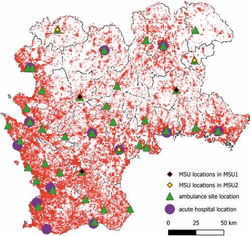
As mentioned above, we considered Sweden’s Southern Health Care Region (SHR), which consists of 49 municipalities located in the four counties of Blekinge, Halland, Kronoberg, and Skåne (see Table A. for more information), and which covers an area of 27.900 square kilometers. The population of SHR was 1.687.000 in 2018, where Malmö (Skåne County), Lund (Skåne County), and Halmstad (Halland County) are the largest populated municipalities with a population of 322.000, 122.000, and 98.800, respectively (Statistics Sweden, 2018). There are 13 acute hospitals equipped with a CT scanner in SHR, and ambulances are located at 39 ambulance sites. Due to the geographical limitation of our study, we chose to not consider islands without fixed connection to the mainland. See Figure 1 for an overview of SHR, where the locations of the ambulance sites and acute hospitals are represented by green triangles and purple circles, respectively. In Figure 1, we also illustrate the population distribution over the region, where the darker the square color is, the higher the population density is.

Figure 1. Overview of SHR, where the green triangles and purple circles represent the locations of ambulance sites and acute hospitals, respectively. The MSUs in the MSU1 and MSU2 scenarios are presented by black and yellow diamonds, respectively. The color of each square displays its population density. The lighter squares have lower density

In 2018, about 3900 stroke cases was registered in southern Sweden, where approximately 20% of the cases were hemorrhagic cases and approximately 80% were ischemic stroke cases. About 20% of the ischemic stroke cases received recanalization therapy, including thrombolysis, both thrombolysis and thrombectomy, or only thrombectomy (The Swedish Stroke Register, 2020). One of the main reasons why about 80% of the ischemic stroke cases do not get treatment is that they arrive too late to the acute hospital. By reducing the time to treatment, recanalization therapy could potentially be given to a much larger share of the ischemic stroke patients.

3.1.2. Scenarios

In our scenario study, we analyzed the possible implications of placing MSUs at different locations in SHR. In particular, we considered three scenarios: A baseline scenario containing only regular ambulances and two extended scenarios containing three MSUs each. The baseline scenario corresponds to the current situation, where regular ambulances are located in all of the 39 ambulance sites shown in Figure 1. The baseline scenario enabled us to identify areas of SHR that are problematic considering the expected time to treatment for stroke patients.

We assumed that all of the 39 ambulance sites located in SHR are candidate locations for MSUs. By visually analyzing the results for the baseline scenario, we created two extended scenarios, which in addition to the regular ambulances, include three MSUs each:

• MSU1: MSUs located in Hörby, Markaryd, and Tingsryd

• MSU2: MSUs located in Lessebo, Hyltebruk, and Kristianstad

In Figure 1, we illustrate the MSU locations in the MSU1 and MSU2 scenarios by black and yellow diamonds, respectively. When we created the two MSU scenarios, we made a tradeoff between the number of MSUs and the coverage of SHR. In particular, we visually analyzed the map in Figure 3a (see Section 5), where we chose to place the MSUs so that they appear to cover as much of the problematic areas, that is, areas with long expected time to treatment, as possible, and not being too close to any acute hospital. The reason for considering scenarios with no more than three MSUs was that this appears to provide decent coverage of SHR; we further took into consideration that the operational costs for an MSU are high.Figure 2

Figure 2. Stroke likelihoods for the considered age groups

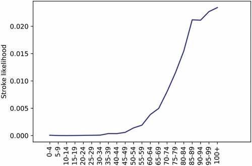
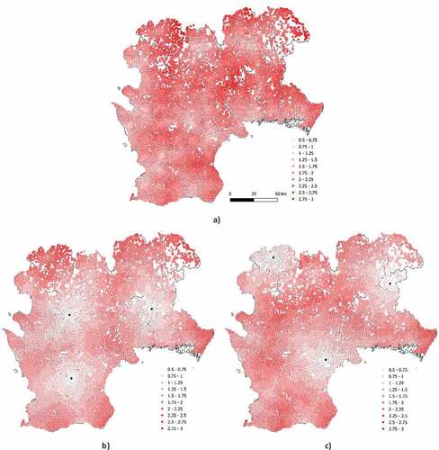
Figure 3. Expected time to treatment for each of the 1$\times$1 km squares covering SHR considering a) only regular ambulances, b) MSU1, and c) MSU2.

In our scenario, we assumed that all dispatches of MSUs or regular ambulances are for actual stroke cases. In addition, due to limitations of the data that was available for our study, we used expert knowledge in order to make the following assumptions:

• It takes three minutes from an emergency call until an ambulance starts driving towards the patient site ($t_l^{AMBRESP}=t_l^{MSURESP}=0,05$h).

• The layover time for both regular ambulances and MSUs is 15 minutes regardless of where the patient is located ($t^{AMBLAY}=t^{MSULAY}=0,25$h).

• The time for diagnosis of a patient inside an MSU is 15 minutes ($t^{MSUDIAG}=0,25\mathrm{h}$).

• The time for diagnosis in hospital is 35 minutes for all of the considered acute hospitals ($t_h^{DIAG}=0,583$h). We based the time for diagnosis in hospital on the door-to-needle time for ischemic stroke patients. To the best of our knowledge, the time to in-hospital thrombolysis is around 30 minutes in SHR. In addition, in a conducted study in a Norwegian stroke centre, the door-to-needle time to thrombolysis treatment was reduced from 27 to 13 minutes (Ajmi et al., 2019). Therefore, we argue that 35 minutes is a quite reasonable time for diagnosis in hospital.

• All of the considered ambulance sites and hospitals are open and provide service on 24/7 basis.

• There is always an ambulance or MSU available when it is needed.

• The MSUs in the two MSU scenarios are able to provide service in the whole region, that is, they are not limited in how far they are able to drive.

• All stroke cases occur at the patients’ homes.

3.1.3. Data processing

We collected the demographic data used in the study from Statistics Sweden (2018) and the age-based stroke data was provided by the Sweden’s Southern Regional Health Care Committee (2018). In addition, we made a geographic division of SHR into a disjoint set of 1$\times$1 km squares (i.e., $R$), as this enabled us to study in detail the variation of demography and the expected time to treatment within SHR.

In order to generate the necessary input for the calculations of the weighted average time to treatment for SHR and for the municipalities in SHR (see Section ‎3), we had to estimate the expected share of stroke cases $Q_r$ for each of the 1$\times$1 km squares $r\in R$ representing SHR. We used the age-based stroke data, together with the demographic data for this aim. The considered stroke data specifies the number of reported stroke cases for 21 age groups over the whole SHR, where we let A = {[0,4), [4,8), …, [95,99), [100, ∞)} denote our disjoint set of age groups. In addition, the demographic data contains the number of inhabitants for each of the age groups and each of the considered 1$\times$1 km squares.

We let $po{p}_{ar}$ denote the number of inhabitants of age group $a\in A$ in square $r\in R$. The total number of inhabitants for age group $a$ in the whole SHR is given by $po{p}_a=\sum _{r\in R}po{p}_{ar}$. For the whole SHR, $S_a$ denotes the number of reported stroke incidents during some specific time period, in our study 2018, for age group $a\in A$. For each of the age groups $a\in A$, we calculated the likelihood that a person will get a stroke during the considered time period as:

(8) $P\left(a\right)=S_a/po{p}_a.$(8)

For each of the considered age groups, we present in Figure 2 the calculated likelihoods, i.e., the $P\left(a\right)$:s, of an individual getting a stroke during one year.

Using the calculated likelihoods, i.e., the $P\left(a\right)$:s, and the $po{p}_{ar}$:s, we calculated the expected number of stroke incidents $S_r$ for each of the subregions $r\in R$ for our considered time period as:

(9) $S_r=\sum _{a\in A}P\left(a\right)\cdot po{p}_{ar}.$(9)

The expected number of stroke cases in the whole region (i.e., SHR) is:

(10) $S=\sum _{r\in R}{S}_r.$(10)

The share of stroke cases that are expected to occur in subregion $r\in R$ is calculated as:

(11) $Q_r=S_r/S.$(11)

Please note that $Q_r$ can be also interpreted as the likelihood that the next stroke in the region will occur in subregion $r$.

We estimated the driving times of both regular ambulances and MSUs using the driving time generation functionality of Open Street Map¹ (OSM), which we accessed using the Openrouteservice toolbox in QGIS. We made our calculations using MATLAB 2019B.

For each of the considered ambulance locations $l\in L$, each of the subregions $r\in R$, and each of the acute hospital $h\in H$, we generated the following driving times:

• $t_{lr}^{AMB\mathrm{\_}LR}$: The estimated time for a regular ambulance to drive from ambulance location $l\in L$ to the centroid $c\left(r\right)$of $r\in R$.

• $t_{lr}^{MSU\mathrm{\_}LR}$: The estimated time for an MSU to drive from ambulance location $l\in L$ to the centroid $c\left(r\right)$of$r\in R$.

• $t_{rh}^{AMB\mathrm{\_}RH}$: The estimated time for a regular ambulance to drive from the centroid $c\left(r\right)$of $r\in R$ to the acute hospital $h\in H$.

It should be noted that OSM generates driving times for cars. As we did not have access to ambulance driving times, we instead estimated the ambulance driving times between different parts of SHR using the generated driving times for cars. In fact, we made a conservative assessment of ambulance driving times. According to ambulance personnel in Southern Sweden (personal report), they are instructed to drive with a safety first principle and will thus keep close to official speed limits. Therefore, we assumed that regular ambulances drive 5% faster than a passenger car, and MSUs drive at the same speed as a car. When we made this assumption, we took into consideration the fact that an MSU equipped with a CT scanner is generally heavier and larger than a regular ambulance; hence, it potentially travels slower.

4. Computational results

In Table 1, we present the weighted and non-weighted average time to treatment for the whole SHR, which we calculated using Equation (4)(4) $t^{TT}=\sum _{r\in R}{t}_r^{TT}\cdot Q_r.$(4) and Equation (5)(5) $t^{TTAVG}=\frac{1}{\left|R\right|}\sum _{r\in R}{t}_r^{TT}$(5) , respectively, for each of our three scenarios. The average, non-weighted, time to treatment for the whole SHR is the mean of expected times to treatment taken over all of the subregions $r\in R$. The expected time to treatment refers to the elapsed time from receiving a call of a stroke case until the treatment is initiated. The weighted average time to treatment for the whole region is the sum of the expected times to treatment taken over all subregions $r\in R$, where the expected time to treatment for subregion $r$ is weighted by $Q_r$, that is, the likelihood that a stroke occurs in subregion $r$. Please see Section 3 for more details. The shortest and longest expected time to treatment for each of the scenarios are presented in Table 2.

Table 1. Weighted and non-weighted average time to treatment for the whole SHR and all of the considered scenarios. Please note that for both non-weighted and weighted average time to treatment, the expected time to treatment is the time from receiving a call until the treatment is initiated. Please see Section 3 for more details

Scenario	Non-weighted average time to treatment	Weighted average to treatment
Baseline	1,62 h	1,33 h
MSU1	1,28 h	1,18 h
MSU2	1,36 h	1,22 h

Table 2. The shortest and longest expected time to treatment for any square for each of the three scenarios

Scenario	Shortest expected time to treatment	Longest expected time to treatment
Baseline	0,91 h (Sjöbo)	2,82 h (Hylte)
MSU1	0,57 h (Hörby)	2,29 h (Uppvidinge)
MSU2	0,56 h (Lessebo)	2,27 h (Vellinge)

In Figure 3, we present for each of our three scenarios, the expected time to treatment for each of the 1$\times$1 km squares of SHR. Please note that the black dots in sub-figures Figure 3(b) and Figure 3(c) of Figure 3 show the locations of the MSUs in the MSU1 and MSU2 scenarios, respectively (see also Figure 1). It should be noted that the lighter the color is in the figures, the shorter the expected time to treatment is for the corresponding square. The results in Figures 3(b) and 3(c) can be also interpreted as how each MSU in each of the two MSU scenarios is expected to impact the expected time to treatment for the different parts of SHR.

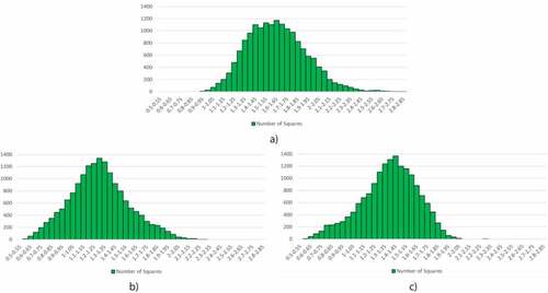
In Figure 4, we illustrate, for each of our three scenarios, how the expected time to treatment is expected to vary for the 1 × 1 km squares covering SHR. It should be noted that the more left-skewed the histogram is, the larger part of SHR is expected to get shorter time to treatment. In particular, this can be seen for MSU2 in Figure 4c. In each of the histograms, the y-axis is the number of squares for each of the 3-minute time to treatment intervals shown on the x-axis.

Figure 4. Histogram showing the distribution of the expected time to treatment over the 1$\times$1 km squares of SHR for a) the baseline scenario, b) MSU1, and c) MSU2.

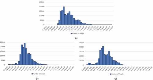
As the histograms in Figure 4 show the number of squares with different expected time to treatment, they do not directly inform about how many of the inhabitants of SHR are expected to get a better situation as a result of placing the MSUs according to our two MSU scenarios. Instead, they inform about the geographic share of the region that is expected to benefit from the use of the MSUs. In Figure 5, we therefore provide histograms showing how the expected time to treatment is distributed over the population of SHR for our three scenarios. The more left-skewed a histogram is, the more stroke patients are expected to receive treatment earlier. In each of the histograms, the y-axis is the number of inhabitants for each of the 3-minute time to treatment intervals shown on the x-axis.

Figure 5. Histogram showing the distribution of the expected time to treatment over the population of SHR for a) the baseline scenario, b) MSU1, and c) MSU2. Each of the bars represents a time interval of 3 minutes (presented in hours)

From the histograms in Figure 5, it is possible to read out the share of inhabitants that are expected to receive treatment within different time thresholds. In order to facilitate the presentation of our results, we provide in Table 3 the share of the total population of SHR (i.e., 1.687.000), that are expected to receive treatment within 60, 75, and 90 minutes for each of the considered scenarios. See also Figure 6, where we present the cumulative distribution function, for each of our three scenarios, of the expected time to treatment for all of the inhabitants of SHR.

Figure 6. Cumulative distribution function, for each of our three scenarios, of the expected time to treatment for the inhabitants of SHR

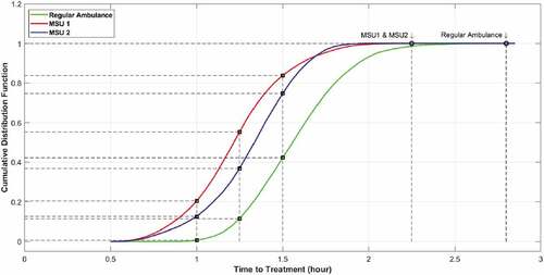
Table 3. Share of the inhabitants in SHR that are expected to receive treatment within 60, 75, and 90 minutes for each of the considered scenarios

Expected time to treatment	Scenario
	Baseline	MSU1	MSU2
$<60$ minutes	3,96%	13,3%	11,7%
$<75$ minutes	47,8%	70,4%	58,5%
$<90$ minutes	80,9%	94,0%	89,5%

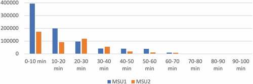
In Figure 7, we show how many of the 1 × 1 km squares in SHR that are expected to get better service after allocating MSUs according to MSU1 and MSU2. According to the chart, the time to treatment is expected to decrease with up to 100 minutes. In the chart, the x-axis is the time interval (in minutes), and the y-axis is the number of squares.

Figure 7. Illustration of how the expected time to treatment is expected to decrease over the 1 × 1 km squares of SHR according to the MSU1 and MSU2 scenarios

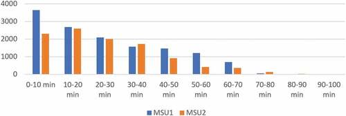
In Figure 8, we show many of the inhabitants of SHR are expected to receive faster treatment as a result of allocating MSUs according to our two MSU scenarios. In other words, we show how the expected time to treatment is expected to be reduced over the population of SHR for the MSU1 and MSU2 scenarios. In the chart, the x-axis is the time interval (in minutes), and the y-axis is the number of inhabitants.

Figure 8. Illustration of how the expected time to treatment is expected to decrease over the population of SHR for the MSU1 and MSU2 scenarios

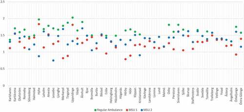
Finally, in Figure 9, we show the average time to treatment for each municipality of SHR in the form of a scatter plot. It can be observed that the MSU1 and MSU2 scenarios are able to provide treatment within 60 minutes for patients living in the municipalities Markaryd, Tingsryd, Eslöv, Hörby, Höör, and Örkeljunga; and Hylte, Lessebo, and Kristianstad, respectively. In Table A, we present the weighted and non-weighted average time to treatment for each of the municipalities and for each of the three scenarios. The weighted and non-weighted average times to treatment for each municipality are calculated using Equation (6)(6) $t_{R{ }^{\mathrm{\prime }}}^{TT}=\sum _{r\in R{ }^{\mathrm{\prime }}}{t}_r^{TT}\cdot \left(\frac{Q_r}{{\sum }_{r\in R{ }^{\mathrm{\prime }}}{Q}_r}\right).$(6) and Equation (7)(7) $t_{R{ }^{\mathrm{\prime }}}^{TTAVG}=\frac{1}{\left|R{ }^{\mathrm{\prime }}\right|}\sum _{r\in R{ }^{\mathrm{\prime }}}{t}_r^{TT}.$(7) , respectively, where $R{ }^{\mathrm{\prime }}$corresponds to the squares of the considered municipality.

Figure 9. Average time to treatment for each municipality of SHR and for each of the three scenarios

5. Discussion

The results of our study suggest that using only a few MSUs, the expected time to treatment is expected to significantly decrease for a large share of the inhabitants in SHR. This is emphasized, e.g., by the calculated weighted and non-weighted average times to treatment for our three scenarios. Compared to the baseline scenario, the average time to treatment dropped from 1,62 h to 1,28 h and 1,36 h, respectively for MSU1 and MSU2. The weighted average time to treatment decreased from 1,33 h to 1,18 h and 1,22 h, respectively for MSU1 and MSU2. The shortest expected time to treatment for any patient in SHR decreased from 0,91 h in the baseline scenario to 0,57 h in MSU1 and to 0,56 h in MSU2, and the longest expected time to treatment was reduced from 2,82 h to 2,29 h in MSU1 and to 2,27 h in MSU2 (see Table 2). In addition, the weighted average time to treatment, which was weighted over the population density, was reduced from 1,33 h to 1,18 h for MSU1 and to 1,22 h for MSU2. It should be emphasized here that the reason that the weighted average time to treatment is much lower than the average time to treatment is that the density of the inhabitants in SHR is higher in those parts that are closer to the ambulance locations and acute hospitals. Visually, this is also shown in Figure 3, where the maps corresponding to MSU1 and MSU2 are much lighter than the map corresponding to the baseline scenario.

By comparing the histograms in Figure 4, it can be further seen that the number of 1$\times$1 km squares with shorter expected time to treatment are significantly higher in the MSU1 and MSU2 scenarios. By comparing the histograms in Figure 5, it can be seen that the number of persons with shorter expected time to treatment is also significantly higher in the MSU1 and MSU2 scenarios. From the figures in these histograms, it is straightforward to read out how large share (or how many) of the population of SHR is expected to receive treatment within a certain time. For example, the share of the population that has an expected time to treatment less than 1 h is 3,96%, 13,3%, and 11,7%, respectively for the baseline, MSU1, and MSU2 scenarios. For 1,25 hours (i.e., 75 min), the figures are 47,8%, 70,4%, and 58,5%, and for 1,5 h (i.e., 90 min), the figures are 80,9%. 94,0%, and 89,5%. Furthermore, for the MSU1 and MSU2 scenarios, 3,35 and 2,96 times as many patients are expected to be treated within 60 minutes compared to the baseline scenario.

According to Figure 7, the inhabitants of 81% and 63% of the 1$\times$1 km squares covering SHR are expected to receive faster treatment according to the MSU1 and MSU2 scenarios, respectively. In addition, the time to treatment of the inhabitants of 63% and 66% of the squares is expected to be reduced up to 30 minutes for MSU1 and MSU2, respectively. Figure 8 shows that the time to treatment is expected to decrease for 82% and 48% of the total population of SHR for the MSU1 and MSU2 scenarios, respectively. In particular, the time to treatment of 84% and 80% of the inhabitants is expected to decrease up to 30 minutes for the MSU1 and MSU2 scenarios, respectively.

It should be noted that the two considered MSU scenarios are two examples of where to locate MSUs. There are other possibilities to place MSUs, but from the results, it can be seen that the different placements of MSUs are expected to lead to benefits for different parts of SHR, which is explicitly shown in Table A, where the weighted and non-weighted average times to treatment are presented for each of the municipalities of SHR. By comparing the results for the two MSU scenarios, we conclude that the MSUs in the MSU1 scenario are expected to improve the situation for a larger share of the population of SHR, whereas the MSUs in the MSU2 scenario are expected to improve the situation for a larger share of those patients which today has the longest time to treatment. The reason for this is most likely that one of the MSUs in MSU1 is located rather close to the Malmö-Lund region, which is the part of SHR with the highest population density. Hence, it is important to carefully consider the trade-off between efficiency and equity when deciding where to place MSUs.

In the present study, we chose to use time for diagnosis. We reasoned that confirmation of a diagnosis of either ischemic or hemorrhagic stroke combining clinical assessment with a CT of the brain is a key decision. In case of an ischemic stroke, treatment with a thrombolytic drug can be started without delay. Furthermore, transportation to a primary or secondary hospital can be planned. If a hemorrhagic stroke is detected, urgent measures like early blood pressure control can be started immediately, and, again, a decision of transportation to a primary or secondary hospital can be made. In trained stroke centers, including those who operate an MSU, the actual additional time from final diagnostic decision to treatment (needle time) is very small and may at most be a few minutes.

6. Conclusions and future work

We have presented a computational study focusing on the potential benefits of using mobile stroke units (MSUs) in Sweden’s Southern health care region (SHR). In particular, we compared the current situation, where regular ambulances, but no MSUs are located at the 39 ambulance sites within SHR, with two extended scenarios, where we added three MSUs in each.

The results of our study show that the time to treatment is expected to significantly decrease for the two MSU scenarios. In particular, we obtained an improvement of about a factor of 3 when considering the share of the population that is expected to receive treatment within an hour, which can be seen in Table 3. The potential benefit of using MSUs can be exemplified by the municipality of Älmhult (with a population of 17.400), where a significant amount of people could be affected by reducing the average time to treatment from 1,9 h to 1,28 h in the MSU1 scenario.

One of the most important strengths of the study is that we divided SHR into a detailed grid of 1$\times$1 km squares, which enabled us to study in detail how the expected time to treatment is expected to vary within SHR. Another strength we want to highlight is that we used a well-established framework to estimate driving times between the different parts of SHR.

In this study, we focused on the time for diagnosis for stroke patients. However, for ischemic stroke patients, which represent the majority of stroke patients, this is the same as studying the time to treatment for those patients who are eligible for thrombolysis, which in this case is the standard treatment and can be initiated almost immediately after the diagnosis. The ischemic patients with larger clots typically benefit from thrombectomy treatment, which is provided only in Lund, in the southwest of SHR. Since the expected benefits of MSUs are significant concerning the time to thrombolysis, it should be emphasized that the expected benefits for thrombectomy patients are even higher owing to the fact that there would be time-savings corresponding to at least part of the driving time from the patient location to the hospital and from the acute hospital to the thrombectomy center plus the acute hospital layover time. Instead, the MSU can drive directly to the thrombectomy center. This is something that should be further investigated in future work. Future work also includes developing an optimization model to solve the search problem of where it is best to place MSUs and to identify a proper trade-off between the equity and efficiency perspectives. It should be further noted that we did not consider co-dispatching of an MSU with a regular ambulance in the presented model. As part of future work, we plan to apply relevant collaborative policies involving MSUs and regular ambulances of ambulance resources to our model.

Financial Disclosure

This work was partially funded by Sweden’s Southern Regional Health Care Committee and The Kamprad Family Foundation for Entrepreneurship, Research & Charity.

Additional information

Funding

We received funding for the research, but we did not have the grant number; please see the section Financial Disclosure.

Notes on contributors

Saeid Amouzad Mahdiraji

Saeid Amouzad Mahdiraji Research interests include simulation, optimization, and machine learning, applied within the health-care logistics domain.

Oliver Dahllöf Research interests are within computer science.

Felix Hofwimmer Research interests are within computer science.

Johan Holmgren Research interests include agent–based simulation and modeling, mathematical optimization, simulation, and machine learning, and his application areas include traffic modeling and health-care logistics.

Radu-CasianMihailescu Research focuses mainly on advances in the field of machine learning, with particular emphasis on deep learning architectures. Key areas of his research also include artificial intelligence, multi-agent systems and smart grids.

Jesper Petersson Has moved from basic experimental studies in the area of cerebrovascular regulation by the endothelium and neurogenic mechanisms to clinical research with main focus on treatment of acute ischemic stroke.

Notes

1. see openstreetmap.org

Appendix

Table A. Weighted and non-weighted average time (in hours) to treatment for all of the municipalities in SHR and all of the considered scenarios

County	Municipa lity	Average time to treatment			Weighted average time to treatment
		Baseline	MSU1	MSU2	Baseline	MSU1	MSU2
Blekinge	Karlshamn	1,37	1,12	1,31	1,13	1,08	1,12
	Karlskrona	1,71	1,55	1,56	1,38	1,33	1,34
	Olofström	1,60	1,31	1,42	1,47	1,35	1,33
	Ronneby	1,67	1,13	1,47	1,44	1,18	1,39
	Sölvesborg	1,46	1,41	1,09	1,41	1,38	1,05
Halland	Halmstad	1,50	1,44	1,23	1,18	1,17	1,13
	Hylte	1,98	1,84	0,88	1,79	1,71	0,77
	Laholm	1,69	1,14	1,62	1,49	1,17	1,46
Kronoberg	Alvesta	1,79	1,53	1,50	1,55	1,44	1,39
	Lessebo	1,71	1,25	0,75	1,58	1,22	0,70
	Ljungby	1,67	1,32	1,48	1,27	1,14	1,20
	Markaryd	1,79	0,82	1,69	1,64	0,71	1,62
	Tingsryd	1,88	0,89	1,23	1,78	0,81	1,22
	Uppvidinge	2,03	1,82	1,33	1,92	1,76	1,28
	Växjö	1,65	1,41	1,25	1,28	1,21	1,12
	Älmhult	1,90	1,28	1,71	1,73	1,26	1,61
Skåne	Bjuv	1,49	1,37	1,49	1,43	1,34	1,43
	Bromölla	1,50	1,45	1,06	1,36	1,35	0,97
	Burlöv	1,27	1,11	1,27	1,27	1,12	1,27
	Båstad	1,53	1,50	1,53	1,52	1,47	1,52
	Eslöv	1,49	0,96	1,43	1,38	0,97	1,36
	Helsing borg	1,32	1,31	1,32	1,19	1,19	1,19
	Hässleholm	1,49	1,14	1,19	1,25	1,09	1,07
	Höganäs	1,37	1,37	1,37	1,34	1,34	1,34
	Hörby	1,65	0,79	1,23	1,47	0,68	1,20
	Höör	1,68	0,90	1,36	1,65	0,82	1,33
	Klippan	1,61	1,21	1,51	1,52	1,20	1,47
	Kristi anstad	1,53	1,23	0,91	1,30	1,16	0,77
	Kävlinge	1,42	1,17	1,42	1,37	1,16	1,37
	Landskrona	1,41	1,33	1,41	1,36	1,33	1,36
	Lomma	1,30	1,13	1,30	1,36	1,16	1,36
	Lund	1,46	1,12	1,46	1,20	1,03	1,20
	Malmö	1,17	1,16	1,17	1,12	1,11	1,12
	Osby	1,82	1,27	1,44	1,63	1,17	1,36
	Perstorp	1,61	1,09	1,44	1,39	1,17	1,35
	Simri shamn	1,82	1,62	1,61	1,76	1,64	1,62
	Sjöbo	1,67	1,06	1,50	1,54	1,04	1,46
	Skurup	1,63	1,48	1,63	1,59	1,49	1,59
	Staffan storp	1,30	1,10	1,30	1,29	1,08	1,29
	Svalöv	1,66	1,31	1,63	1,57	1,28	1,55
	Svedala	1,48	1,30	1,48	1,39	1,27	1,39
	Tomelilla	1,62	1,34	1,39	1,45	1,30	1,30
	Trelleborg	1,58	1,50	1,58	1,40	1,38	1,40
	Vellinge	1,40	1,37	1,40	1,48	1,41	1,48
	Ystad	1,41	1,38	1,41	1,22	1,22	1,22
	Åstorp	1,37	1,19	1,37	1,34	1,18	1,34
	Ängelholm	1,32	1,21	1,32	1,09	1,08	1,09
	Örkeljunga	1,76	0,93	1,61	1,68	0,91	1,56
	Östra Göinge	1,58	1,40	1,16	1,48	1,38	1,07

References

- Ajmi, S. C., Advani, R., Fjetland, L., Kurz, K. D., Lindner, T., Qvindesland, S. A., Ersdal, H., Goyal, M., Kvaløy, J. T., & Kurz, M. (2019). Reducing door-to-needle times in stroke thrombolysis to 13 min through protocol revision and simulation training: A quality improvement project in a Norwegian stroke centre. British Medical Journal Quality & Safety, 28(11), 939–18. https://doi.org/10.1136/bmjqs-2018-009117
- Al Fatah, J., Alshaban, A., Holmgren, J., & Petersson, J. (2018). An agent-based simulation model for assessment of prehospital triage policies concerning destination of stroke patients. Procedia Computer Science, 141, 405–412. https://doi.org/10.1016/j.procs.2018.10.183
- Cerejo, R., John, S., Buletko, A. B., Taqui, A., Itrat, A., Organek, N., Cho, S. M., Sheikhi, L., Uchino, K., Briggs, F., Reimer, A. P., Winners, S., Toth, G., Rasmussen, P., & Hussain, M. S. (2015). A mobile stroke treatment unit for field triage of patients for intraarterial revascularization therapy. Journal of Neuroimaging, 25(6), 940–945. https://doi.org/10.1111/jon.12276
- Dahllöf, O., Hofwimmer, F., Holmgren, J., & Petersson, J. (2018). Optimal placement of mobile stroke units considering the perspectives of equality and efficiency. Procedia Computer Science, 141, 311–318. https://doi.org/10.1016/j.procs.2018.10.195
- Ebinger, M., Winter, B., Wendt, M., Weber, J. E., Waldschmidt, C., Rozanski, M., Kunz, A., Koch, P., Kellner, P. A., Gierhake, D., Villringer, K., Fiebach, J. B., Grittner, U., Hartmann, A., Mackert, B.-M., Endres, M., & Audebert, H. J. (2014). Effect of the use of ambulance-based thrombolysis on time to thrombolysis in acute ischemic stroke: A randomized clinical trial. Journal of the American Medical Association, 311(16), 1622–1631. https://doi.org/10.1001/jama.2014.2850
- Holodinsky, J. K., Patel, A. B., Thornton, J., Kamal, N., Jewett, L. R., Kelly, P. J., Murphy, S., Collins, R., Walsh, T., Cronin, S., Power, S., Brennan, P., O’hare, A., McCabe, D. J., Moynihan, B., Looby, S., Wyse, G., McCormack, J., Marsden, P., Harbison, J., & Williams, D. (2018). Drip and ship versus direct to endovascular thrombectomy: The impact of treatment times on transport decision-making. European Stroke Journal, 3(2), 126–135. https://doi.org/10.1177/2396987318759362
- Mathur, S., Walter, S., Grunwald, I. Q., Helwig, S. A., Lesmeister, M., & Fassbender, K. (2019). Improving prehospital stroke services in rural and underserved settings with mobile stroke units. Frontiers in Neurology, 10, 10. https://doi.org/10.3389/fneur.2019.00159
- Phan, T. G., Beare, R., Srikanth, V., & Ma, H. (2019). Googling location for mobile stroke unit hub in metropolitan Sydney. Frontiers in Neurology, 10, 810. https://doi.org/10.3389/fneur.2019.00810
- Reimer, A. P., Zafar, A., Hustey, F. M., Kralovic, D., Russman, A. N., Uchino, K., Hussain, M. S., & Udeh, B. L. (2020). Cost-consequence analysis of mobile stroke units vs. standard prehospital care and transport. Frontiers in Neurology, 10, 1422. https://doi.org/10.3389/fneur.2019.01422
- Rhudy Jr., J. J. P., Alexandrov, A. W., Rike, J., Bryndziar, T., Maleki, A. H. Z., Swatzell, V., Dusenbury, W., Metter, E. J., & Alexandrov, A. V. (2018). Geospatial visualization of mobile stroke unit dispatches: A method to optimize service performance. Interventional Neurology, 7(6), 464–470. https://doi.org/10.1159/000490581
- Sarraj, A., Savitz, S., Pujara, D., Kamal, H., Carroll, K., Shaker, F., Reddy, S., Parsha, K., Fournier, L. E., Jones, E. M., Sharrief, A., Martin-Schild, S., & Grotta, J. (2020). Endovascular thrombectomy for acute ischemic strokes: current US access paradigms and optimization methodology. Stroke, 51(4), 1207–1217. https://doi.org/10.1161/STROKEAHA.120.028850
- Schlemm, L., Ebinger, M., Nolte, C. H., & Endres, M. (2018). Impact of prehospital triage scales to detect large vessel occlusion on resource utilization and time to treatment. Stroke, 49(2), 439–446. https://doi.org/10.1161/STROKEAHA.117.019431
- Statistics Sweden (2018) demographic data 2018. https://www.scb.se/
- Sweden’s Southern Regional Health Care Committee (2018) stroke data 2018. https://sodrasjukvardsregionen.se/
- The Swedish Stroke Register (2020) Stroke registrations. https://www.riksstroke.org/sve/forskning-statistik-och-verksamhetsutveckling/statistik/registreringar/
- Walter, S., Grunwald, I. Q., Helwig, S. A., Ragoschke-Schumm, A., Kettner, M., Fousse, M., Lesmeister, M., & Fassbender, K. (2018). Mobile stroke units-cost-effective or just an expensive hype? Current Atherosclerosis Reports, 20(10), 49. https://doi.org/10.1007/s11883-018-0751-9
- World Stroke Organization (2019) Facts and figures about stroke. https://www.world-stroke.org/world-stroke-day-campaign/why-stroke-matters/learn-about-stroke/
- Zhao, H., Coote, S., Easton, D., Langenberg, F., Stephenson, M., Smith, K., Bernard, S., Cadilhac, D. A., Kim, J., Bladin, C. F., Churilov, L., Crompton, D. E., Dewey, H. M., Sanders, L. M., Wijeratne, T., Cloud, G., Brooks, D. M., Asadi, H., Thijs, V., Chandra, R. V., & Davis, S. M. (2020). Melbourne mobile stroke unit and reperfusion therapy: greater clinical impact of thrombectomy than thrombolysis. Stroke, 51(3), 922–930. https://doi.org/10.1161/STROKEAHA.119.027843