
 ?Mathematical formulae have been encoded as MathML and are displayed in this HTML version using MathJax in order to improve their display. Uncheck the box to turn MathJax off. This feature requires Javascript. Click on a formula to zoom.
Abstract
An integrated linear regression technique was developed and validated to model dissolved oxygen in salt lakes by using R software and based on data from Sawa Lake, Iraq. The technique helps understand and evaluate salty aquatic ecosystems in the presence of water quality data gaps. The technique involved selecting the important water quality parameters that have significant statistical relationship with dissolved oxygen. In order to make the regression development simpler, the validation approach was incorporated with the model. Linearity, homogeneity, normality, outliers, and influential data points were verified. The simulation approach was also capable of displaying the interaction between the selected water quality parameters and the other insignificant parameters. The statistical analysis results indicated that dissolved oxygen in salt lakes is a function of total dissolved solids. The developed model represented dissolved oxygen with R-squared of 90.73% and p-value of 1.08E-06. Furthermore, the model results showed that the influence of salty ions on dissolved oxygen/total dissolved solids model is the same. It was found that temperature has a significant impact on the developed dissolved oxygen model. In addition, the model simulation revealed that salt melting surrounding the lake due to temperature variation during the year cycle increased total dissolved solids in the lake water. Consequently, the lake dissolved oxygen levels were impacted.
Public interest statement
In future, salt lakes will be considered one of the main water resources in the under-developed and developed countries due to water issues. These lakes are not protected well, and need to be preserved for future human essentials. In this work, the implemented statistical modelling technique highlights a visual and quantitative way to be used for salt lakes protection. Since dissolved oxygen is a measure of lake health, the proposed model is capable of simulating dissolved oxygen in salt lakes by using total dissolved solids only. Integrated water quality data are not available for all lakes, especially in poor countries. Using the current statistical technique helps researchers monitor their public water resources in case of data gap or insufficient data. Hence, the present paper revealed insight of the issue and developed the solution for the public necessities.
1. Introduction
Salt or saline lakes are interesting inland features and need to be taken into account in water quality modelling since many water quality parameters (environmental variables) can be changed due to environmental conditions such as dissolved oxygen, water temperature, and even salt compositions. Similarly, climate change and global warming can affect salt lakes ecosystems (Hussain & Abed, Citation2019; Tweed et al., Citation2011). Salinity impacts the water cycle by affecting the evaporation process in lakes (Obianyo, Citation2019). Unfortunately, very few water quality studies have been conducted on salt lakes compared to freshwater lakes even though inland salt water has approximately the same volume as freshwater rivers and lakes (Last, Citation2002).

It is not surprising that salt lakes in underdeveloped countries have even less attention than in developed countries, especially those countries that have problems with water resources and less data to work on. One of these salt lakes is Sawa Lake, located in Iraq about 26.74 km west of Samawah City (N 31°18´ and E 45°00´). It has almost no attention and no monitoring system, and it is not protected. Concerns that future changes of climate or management may affect the lake water quality have promoted the need for modeling the lake for future predictions. Shope and Angeroth (Citation2015) highlighted the need for more monitoring of dissolved oxygen in salt lakes statistically. Salt lakes represent about 45% of the total inland lake volume (Shiklomanov, Citation1990), and they are used as a source for water supply especially in regions of dry/hot weather and low groundwater level. Sawa lake is a good example for this. The lake significance is that its located is within a desert area where people have used wells for water supply. This concern makes salt lakes valuable for humans.
Sawa Lake is located within a gypsum region, and it does not have any inflows or outflows. The only ways to gain or lose water are by rainfall, evaporation, or groundwater. Some algae species, phytoplankton, and a few kinds of fish exist (Awadh & Muslim, Citation2014; Hassan et al., Citation2006). Hence, fish species need to be preserved in the lake to meet the human essentials (Cordier et al., Citation2020; Moayedi et al., Citation2019). The most important element in aquatic ecosystems is oxygen because it is necessary for life, controls many chemical reactions through oxidation, and gives a general indication of aquatic systems health (Cole & Wells, Citation2006). However, the Sawa Lake water quality monitoring has ignored the role of dissolved oxygen in the lake ecosystem. Questions such as how dissolved oxygen in Sawa Lake relies on other water quality variables statistically have not been answered. In other words, exploring how statistically significant the relationship between dissolved oxygen and the other variables is important. By answering this question, water quality in the lake can be statistically related to easily measured water quality variables to predict the impact on dissolved oxygen.
Zhang (Citation2019) illustrated the global trends and the most common approach used in water quality assessment, the Water Quality Index (WQI). For instance, Mohammed and Abdulrazzaq (Citation2018) conducted a case study to assess the water quality using the WQI approach. However, the modelling chosen for this study is a simple statistical model based on field data since the lake has not properly been inspected based on the latest water quality modelling techniques, especially by the statistical methods. Thus, the need to develop a statistical dissolved oxygen model for Sawa Lake arises based on the following issues. First, Sawa Lake location is in Iraq, which is a developed country. Water resources in Iraq are not protected and managed, and need extensive studies in order to re-preserve the aquatic systems. In addition, integrated data that are necessary for developing a full-scale numerical model capable of simulating all of the environmental processes are not available completely. Data such as bathymetry maps, continuous time series for the water quality parameters (historical data), inflows, outflows, and meteorological data are required during the same time period in order to develop a water quality model. Second, there is need to provide a statistically proven and robust technique capable of selecting the most environmental variables that impact dissolved oxygen in salt lakes. Finally, salt lake ecosystems have high salt concentrations with different kinds of ions. Each ion concentration can be explored efficiently by taking the advantages of R software packages (R Core Team, Citation2015), making the dissolved oxygen depletion in the lake clear by knowing the contribution of each salt ion in the total dissolved solids. Hence, this research outlines an efficient statistical technique for modelling dissolved oxygen by using R software packages. The adopted visual approach is based on statistical hypotheses tests, and results in a linear regression model that governs the relationship between the dominant environmental predictor variables and dissolved oxygen (the dependent variable).
The contribution of this work is to develop and validate a statistical technique capable of determining the relationship between dissolved oxygen and the other water quality parameters for salt lakes by using R software. Therefore, the main objectives of this research are to build a linear regression for modelling dissolved oxygen based on the available water quality parameters from Sawa Lake, valid the model statistically, and visualize the model by showing the interaction between the model and the unimportant water quality parameters.
2. Materials and methods
2.1. Study area, data description, and model specification
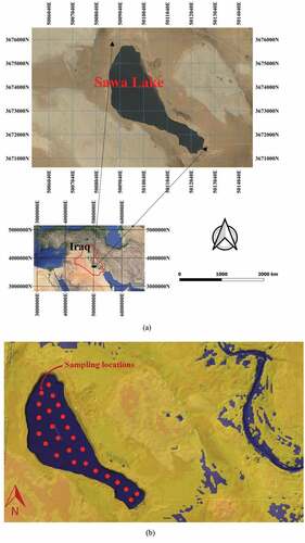
The Sawa Lake area is approximately 5.1 km2, and the bottom elevation is about 17 m above sea level with water depth of about 3.0–5.5 m. The lake water level elevation is higher than the surrounding area level by approximately 2–5 m (Ziyadi et al., Citation2015). Monthly samples of water were taken from Sawa Lake in 2017 by the Iraqi Ministry of Health and Environment for water quality monitoring purposes. The monitoring system included taking the average of 25 samples every mid-month between 9 and 11 am for evaluating the water quality in the lake. shows the study area and sampling locations used in this study.
Figure 1. The area of study; (a) Sawa Lake region retrieved by QGIS, and (b) Map of Sawa Lake retrieved from Landsat 8 OLI/TIRS Level-2 Data Products (WRS path/row: 168/038; acquired on 3 June 2017), showing the locations of samples used in this study
Many water quality parameters were measured monthly during the study period. Dissolved Oxygen (DO), pH, Total Dissolved Solids (TDS), Total Suspended Solids (TSS), Sulfate (SO4), Chloride (Cl), Nitrate (NO3), Calcium (Ca), Magnesium (Mg), Sodium (Na), Electrical Conductivity (EC), Fluoride (F), Potassium (K), Turbidity (Turb), and Total Hardness (T.H) were the available water quality variables used as the raw dataset (see ).
Table 1. Monthly averaged water quality parameters of Sawa Lake in 2017
Since the aim of this research was to investigate whether a statistically significant linear relationship exists between the response variable (DO) and the other fifteen environmental predictors, DO was considered the dependent variable and the other predictors were the independent variables. The model goal was to describe DO concentration based on the other water quality parameters so that DO in Sawa Lake can be predicted by other parameters. Accordingly, the target linear regression model expresses DO as a function of other water quality predictors that have a significant relationship with DO.
2.2. The conceptual framework of the study
To systematically accomplish the data analyses, several regression models needed to be built successively by removing predictor variables that are not important. These analyses included testing the null hypothesis that DO is not affected by the other model variables (DO varies independently of the other model variables) against the alternative hypothesis that DO dependents on the other variables significantly. All statistical analyses were performed in R 3.1.3 (R Core Team, Citation2015) and based on the statistical analysis in Gotelli and Ellison (Citation2013). The general framework of the analyses was summarized in , which is the conceptual model of the study.
Figure 2. Statistical conceptual model
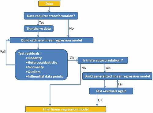
By running this statistical conceptual model, the relationship between DO and the other water quality predictors was determined whether it is statistically significant or not by exploring and answering the following hypotheses statistically:
- Null hypothesis: There is no significant relationship between DO and the other water quality predictors (the linear regression line slope = 0).
- Alternative hypothesis: There is a significant relationship (the linear regression line slope ≠ 0).
Initially, the null hypothesis was assumed true to be checked through the model by using statistical tests in order to make the final decision (true or false hypothesis).
3. Results and discussion
3.1. The predictor variables selection approach
First of all, and in order to make a decision and decide which predictor variables need to be tested for the linear regression model, the data relationships were explored before building the model. This initial look based on the understanding of the system is an important step prior to developing the linear regression model (Burnham and Anderson, Citation2002; Zuur et al., Citation2010).
(a) shows a graphical representation (scatterplot matrix) summarizing the relationships between each pair of variables in the raw data. There are many interesting relationships that can be recognized based on the trend between DO (the response variable) and the other water quality parameters (the predictor variables), but no decision can be made until a statistical evidence exists. In addition, the data were graphically displayed as shown in (b and c), which are correlation matrix plots for the available water quality parameters in two different ways. In both plots, the lower/left panels display the pairwise Pearson correlation coefficients (0–1) between variables, while the upper/right panels use colors to display the coefficients in which the color intensity and the circle size are proportional to the correlation coefficient. Displaying the water quality parameters in such a way helps detect how the parameters are strongly correlated among themselves. The strong correlation between any two predictors means there is collinearity (also called multicollinearity), leading to a non-significant relationship in the target multiple regression model (Gotelli & Ellison, Citation2013; Zuur et al., Citation2010, Citation2009).
Figure 3. Correlation plots (a, b, and c) of Sawa Lake data; (a) Scatterplot matrix of Sawa Lake data, (b) Correlation color matrix of Sawa Lake data, and (c) Correlation pie plots of Sawa Lake data
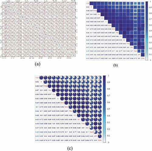
Because this research was interested in finding a significant relationship between DO as a response variable and other predictors. Temperature, TDS, and turbidity were assumed to be the main predictors to explain the variation in the response variable DO and to start with developing the regression model because the other predictors are salts and already are accounted for in TDS and Turbidity. This assumption will be proven statistically significant while building the model. Therefore, the correlation between these three predictors was explored. For example, it can be clearly noticed that all predictors have a strong correlation with Temp except Turb with a correlation coefficient of 0.56 (the lowest coefficient). Thus, we expect to get a confusing statistical analysis if the linear regression model was built based on Temp and all other predictors due to these strong correlation coefficients (≥0.74) and a good regression if the linear regression model was built based on Temp and Turb only. Same idea could be applied to TDS and Temp with cautious.
A graphical summary (boxplots) of the three variables is provided in (a), and the corresponding correlation matrix was plotted as shown in (b). Even though Turb data statistically reveal outliers presence, the outliers will be kept because they did not come from errors or mistakes during sample collection such as errors due to parameter measurements or calculations, or any other source that may change the real values. It was found that based on old observations the turbidity in the lake has minimum values in March. Furthermore, to improve the response variable normality due to data spread in addition to reduce the outliers effect on the predictors, the log transformation of the variables DO, Temp, Turb, and TDS was considered in the regression model building.
Figure 4. Boxplots and correlation matrix of dissolved oxygen, temperature, and turbidity in 2017 extracted from Sawa Lake raw data; (a) Dissolved oxygen, temperature, and turbidity boxplots from Sawa Lake data in 2017, and b) Dissolved oxygen, temperature, and turbidity correlation matrix from Sawa Lake data in 2017
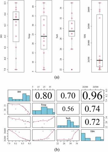
Based on the correlation between the response variable and the predictors as shown in (b), DO has a strong correlation with TDS (a correlation coefficient of 0.96) and has a good correlation with Temp and Turb (a correlation coefficient of 0.8 and 0.7, respectively). For the predictors, TDS has a good correlation with Temp and Turb (a correlation coefficient of 0.74 and 0.72, respectively). Therefore, the presence of TDS with Temp and Turb in the same model could lead to collinearity or non-significant relationship. On the other hand, Temp and Turb could be together in the same model due to the low correlation between them (a correlation coefficient of 0.56).
Therefore, it was necessary to try building the linear regression model based on (trial 1: DO, Temp, and Turb) and (trial 2: DO and TDS) to avoid the multicollinearity issue and to make sure that the predictor variables behave independently. Then, a step-wise forward selection was carried out to include other predictors as long as they can contribute in explaining DO statistically.
3.2. The linear regression model development and validation
A full regression model was fitted between the response variable (logDO) and the other water quality predictors (logTemp, logTurb, and logTDS). It was found that keeping TDS leads to a non-significant relationship (the null hypothesis is true). Removing TDS, therefore, adjusted the regression and made the null hypothesis rejected. The statistical summary of the final model is shown in , after excluding TDS. The regression outputs show the estimated intercept and slopes in addition to the standard errors, t-values and p-values. There is also information on the multiple R-squared, the adjusted R-squared, and F-statistic. The adjusted R-squared was 0.6242, referring to the relationship strength between the response variable and the predictors in which 62.42% of the variance in DO can be explained by Temp and Turb. Setting the typical choice 5% confidence interval (Zuur et al., Citation2009), the p-value of the intercept and the slopes were less than the 5% significance level, confirming that the null hypothesis (slope = 0) is not true and the relationship between the response variable and the predictors is significant. In addition, the regression as a whole model is performing well since the F-statistic indicated that the p-value is less than the 5% significance level. In other words, the null hypothesis was rejected and the alternative hypothesis was true. As a result, the estimated linear regression model gave the following multiple linear regression model, EquationEq. (1)(1)
(1) :
Table 2. The full linear regression model summary statistics of Equationequation 1(1)
(1)
where log is the natural logarithms.
The linear regression of EquationEq. (1)(1)
(1) was based on the trial 1 (the full model includes DO, Temp, and Turb). Doing trial 2, the linear regression analysis gave another robust model (EquationEq. (2
(2)
(2) )), see for the statistical summary of (EquationEq. (2)
(2)
(2) ):
Table 3. The full linear regression model summary statistics of Equationequation 2(2)
(2)
Both of the above linear regression models need to be verified to determine whether or not the model that has been built meets the linear regression underlying assumptions. Non-linearity, heteroscedasticity (violation of homogeneity), non-normality, outliers, and influential data points must be tested (Gotelli & Ellison, Citation2013; Zuur et al., Citation2016, Citation2009).
Hence, missing the important assumption such as the predictor variables interdependency and the residual patterns absence produces biased parameter estimates and type I errors (Quinn and Keough, Citation2002). In addition, autocorrelation in data should be taken into account by assessing the residuals independence using either or both of the autocorrelation functions and/or variograms (Schabenberger & Pierce, Citation2001). Therefore, a diagnostic test was conducted to test both models.
(a) includes the multiple regression model validation graphs obtained by applying the multiple linear regression (EquationEq. (1(1)
(1) )) on the Sawa Lake data. These graphs are typical linear regression outputs, produced in R, and used to validate the linear regression (Zuur et al., Citation2009). The graphs were arranged in four panels:
Figure 5. Linear regression validation graphs; (a) Model validation graphs of .EquationEq. 1(1)
(1) , and (b) Model validation graphs of EquationEq. 2
(2)
(2)
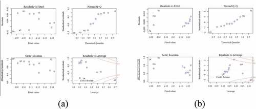
The upper left panel shows the residuals (fitted values minus observed values) against fitted values. It is used to assess the homogeneity assumption. If there is a pattern or different scatter in the spread of the residuals around the horizontal line (zero residuals), the homogeneity assumption will be violated due to the non-linearity, and therefore the residuals will scatter around the center line differently. Based on this panel outputs, the residuals bounce around the horizontal line (the mean of the residuals is zero) with no systematic patterns. Thus, the homogeneity assumption is valid. However, the presence of minor violation in homogeneity is not a major problem to be considered (Sokal & Rohlf, Citation1995).
The upper right panel shows the standardized residuals, which is obtained by taking the absolute value and weighted by the leverage, against the theoretical quantiles to check the normality assumption graphically. The points follow the 1:1 line except at the tails. Therefore, Shapiro-Wilk normality test was used to test the residuals statistically to prove the normality assumption clearly (Gotelli & Ellison, Citation2013). Based on the Shapiro-Wilk test results, the residuals distribution is normal (the null hypothesis) because of the large value of w-value and p-value >0.05 significance level.
The lower right panel shows the square-root transformed standardized residuals against the fitted values to check the equal variance assumption graphically. No pattern exists; however, the F-test based on the residuals was used to check the equal variance assumption too. All residuals were divided into two groups based on the fitted values median, and then the two groups were tested for equal variances (σ1,σ2) by assuming true equal variances (the null hypothesis: σ1/σ2 = 1, and the alternative hypothesis: σ1/σ2 ≠ 1). The F-test resulted in a p-value >0.05 significance level in addition to F-value (σ1/σ2 ≠ 1). Therefore, the null hypothesis is not true and the two variances are different. Because of the good p-value (greater than 0.05 significance level), the linear regression model meets the assumption of equal variance.
Finally, the lower right panel was used to check the influential outliers based on Cook’s distance. The third data point has a Cook’s distance greater than 1. Therefore, this data point is an influential point (Fox, Citation2015; Hair et al., Citation1998; Zuur et al., Citation2009). It was found that removing this data point from the raw data and repeating the analysis lead to a non-significant relationship between DO and the other predictors. Thus, the model of EquationEq. (1)(1)
(1) was rejected due to this violation, and the model of EquationEq. (2)
(2)
(2) should be considered to be examined.
Basically, EquationEq. (2)(2)
(2) is a simple linear regression model. (b) shows the related model validation graphs. It is clear that all graphs were improved as we moved from EquationEq. (1)
(1)
(1) to EquationEq. (2
(2)
(2) ), meeting all of the assumptions of the linear regression, see for the statistics. However, time independency needs to be checked.
Table 4. Regression models and summary statistics
3.3. The auto-correlation effect
Because the dataset that was used to model Sawa Lake was time series, auto-correlation (time dependency) could be statistically significant. The presence of auto-correlation will influence the final model functionality and could lead to wrong predictions if ignored. It was noticed that the regression p-value may be overestimated by 400% in the presence of ignored auto-correlation (Ostrom, Citation1990). In order to assess the temporal aspects, auto-correlation function (ACF) can be used to evaluate independence of residuals in case of constant time resolution (Schabenberger & Pierce, Citation2001). Zuur et al. (Citation2009) considered ACF the more formal visualization tool to detect patterns. An ACF value represents the Pearson correlation between a time series and the same time series shifted by one time space, called time lag (the time resolution in this case). shows the autocorrelation plots for the model of EquationEq. (1)(1)
(1) and EquationEq. (2
(2)
(2) ), respectively, indicating clearly that there is no significant auto-correlation because ACFs are within 95% confidence levels (the blue dash lines).
Figure 6. Model auto-correlation plots
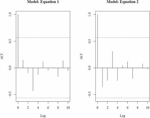
Thus, EquationEq. (2)(2)
(2) model satisfies the linear regression assumptions graphically and statistically and can be used to describe DO in Sawa Lake where 90.73% of the variance in DO can be explained by TDS. Hence, the target null hypothesis that there is no significant relationship between DO and the other environmental predictors was rejected, and the alternative hypothesis that there is significant relationship was accepted.
3.4. The linear regression model simulation
In order to make future predictions for specific environmental management purposes, it is necessary to explore the model comparability with the original data (Gelman et al., Citation2013; Zuur et al., Citation2013). First of all, the final model in EquationEq. (2)(2)
(2) was plotted using the Sawa Lake raw data as shown in (a). There is good agreement between the model predictions and data, reflecting the strong relationship between DO and TDS in Sawa Lake since 90.73% in the DO variance can be expressed in terms of TDS with a low p-value.
Figure 7. Comparisons between the model predictions with raw data; (a) DO in Sawa Lake by fitting the model of EquationEq. 2(2)
(2) to the raw data in 2017, and (b) The interaction among dissolved oxygen, temperature, and turbidity, the circle size was scaled by the relevant temperature
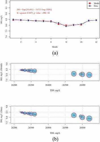
TDS caused oxygen depletion in Sawa Lake, mainly during summer conditions. Shope and Angeroth (Citation2015) reported same depletion situation in Great Salt Lake, US. The DO started dropping on June and recovered on November, keeping around the same value during the rest of the year approximately. Finally and by taking the advantages of the model in EquationEq. (1(1)
(1) ), the DO had a strong correlation with Temperature too. Therefore, the plots in (b) were used to reveal the interaction among DO, TDS, and Temp based on the original data and the valid model in EquationEq. (2)
(2)
(2) . The circle size is proportional to Temp. Hence, the model DO predictions showed same pattern as the data, in which the highest TDS value occurred on August when the water temperature was the highest, resulting in the low DO level. Thus, the model in EquationEq. (2)
(2)
(2) was proven statistically and graphically in addition to the comparability with the data.
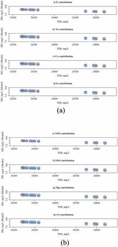
In addition, the salty ions that contribute to TDS and affect DO were explored. Plotting DO against TDS and taking into account these ions effect fulfilled this purpose. The graphs (a to h) in highlight the ions effect on the relationship between DO and TDS. Interestingly, all of the salty ions have almost the same influence on DO and TDS relationship as shown by the circles sizes in the graphs (a to h). The circles sizes are bigger during summer season, however. This underlies the impact of temperature on the undertaken melting processes surrounding the lake region. Although this supports the present analysis result that the most influential environmental variable on DO after TDS is the Temp as shown in the rejected model of EquationEq. (1(1)
(1) ), it shows a statistically insignificant relationship. Hence, comparing with helps identify that the DO drop down during summer season was due to a TDS increase in the lake as a result of the high temperature. Ions move faster when the water is warm. The high temperature increased the amount of TDS in salt lakes due to melting process and led to more DO depletion in the same time. Al-Zubaidi and Wells (Citation2020) and Al-Zubaidi (Citation2018) stated the role of temperature in modelling dissolved oxygen in freshwater analytically and numerically. However, TDS can be used to predict dissolved oxygen levels in salt lakes statistically.
Figure 8. The contribution of ionic compounds (a-h) to TDS and how they impact DO, the circle size was scaled by the relevant ion concentration
4. Conclusions
A new statistical technique was developed in order to model dissolved oxygen in a small salt lake called Sawa Lake, located in Iraq. The findings of this research indicated that:
The statistical approach can model the salt lake aquatic ecosystem or similar in underdeveloped and developed countries such as Iraq where complete data are not available for the numerical models to be used. It was capable of showing the interaction between the water quality variables visually and statistically, revealing the correlation strength between the environmental predictors.
The technique was also capable of building a linear regression based on statistical diagnostic tests. Therefore, the model selects just the environmental predictors that have a statistically significant relationship with the dependent variable rather than building a full model based on all the environmental predictors. Furthermore, a visual way was proposed to show the contribution of the environmental predictors that were not selected in this relationship by showing the impact of those predictors on the model.
It was found that the dissolved oxygen in the lake is a function of the total dissolved solids only with R-squared of 90.73% and p-value of 1.08E-06. Therefore, 90.73% of the variance in dissolved oxygen can be expressed by total dissolved solids.
The statistical model developed in this study showed that all salty ions have a similar interaction with the dissolved oxygen/total dissolved solids relationship. In contrast to the salty ions, the results showed that temperature variation with time was the most water quality variable that plays a major role in the dissolved oxygen/total dissolved solids relationship. Thus, during summer season, lake temperature goes up, reducing lake dissolved oxygen due to the higher total dissolved solids coming into the lake through salt melting processes in the lake region.
Notations
SymbolDefinition
DODissolved oxygen
pHPotential of hydrogen
TDSTotal Dissolved Solids
TSSTotal Suspended Solids
SO4Sulfate
ClChloride
NO3Nitrate
CaCalcium
MgMagnesium
NaSodium
ECElectrical Conductivity
FFluoride
KPotassium
TurbTurbidity
T.HTotal hardness
σ 1Variance of group 1
σ 1Variance of group 2
ACFAuto-correlation function
Acknowledgements
The authors thank the department of Environmental Engineering, Faculty of Engineering, University of Babylon, Iraq for support this research. Also, many thanks to Dr Scott A. Wells (Department of Civil and Environmental Engineering, Portland State University, US) for his notes.
Additional information
Funding
Notes on contributors

Hussein A. M. Al-Zubaidi
Hussein A. M. Al-Zubaidi is Assist. Prof. Dr. and the Head of Environmental Engineering Department at the Faculty of Engineering, University of Babylon, Iraq. He received his B.Sc. degree in Civil Engineering from the College of Engineering, University of Babylon, Iraq and M.Sc. degree in Environmental Engineering from the same College in 2003 and 2007, respectively. The author finished his Ph.D. degree in Civil and Environmental Engineering at Portland State University, Oregon, USA in 2018 under the supervision of Prof. Dr. Scott A. Wells. He has worked as a research assistant at the Department of Environmental Engineering, University of Babylon since 2005 and has become the department head since 2020. His research interests are working on environmental modelling (analytical, statistical, and numerical methods), water and wastewater treatment, and environmental engineering. Also, Hussein has published more than 20 papers in reputed journals and has been serving as a reviewer for different reputable journals.
References
- Al-Zubaidi, H. A. M., 2018. 3D Hydrodynamic, Temperature, and Water Quality Numerical Model for Surface Waterbodies: Development, Verification, and Field Case Studies. Dissertations and Theses. Paper 4500. https://doi.org/10.15760/etd.6384
- Al-Zubaidi, H. A. M., & Wells, S. A. (2020). Analytical and field verification of a 3D hydrodynamic and water quality numerical scheme based on the 2D formulation in CE-QUAL-W2. Journal of Hydraulic Research, 58(1), 152–18. https://doi.org/10.1080/00221686.2018.1499051
- Awadh, S. M., & Muslim, R. (2014). The formation models of gypsum barrier, chemical temporal changes and assessments the water quality of Sawa Lake, Southern Iraq. Iraqi Journal of Science, 55(1), 161–173. https://www.iasj.net/iasj/article/86984
- Burnham, K. P., & Anderson, D. R. (2002). Model selection and multimodel inference: A practical information-theoretic approach., 2nd ed. Springer, New York
- Cole, T. M., & Wells, S. A. (2006). CE-QUAL-W2: A two-dimensional, laterally averaged, hydrodynamic and water quality model, Version 3.5. Instruction Report EL-06-1, US Army Engineering and Research Development Center. http://archives.pdx.edu/ds/psu/12049
- Cordier, C., Guyomard, K., Stavrakakis, C., Sauvade, P., Coelho, F., & Moulin, P. (2020). Culture of microalgae with ultrafiltered seawater: A feasibility study. SciMedicine Journal, 2(2), 56–62. https://doi.org/10.28991/SciMedJ-2020-0202-2
- Core Team, R. (2015). R: A language and environment for statistical computing. //www.R-project.org.
- Fox, J. (2015). Applied regression analysis and generalized linear models. Sage Publications.
- Gelman, A., Carlin, J., Stern, H., Dunson, D., Vehtari, A., & Rubin, D. (2013). Bayesian data analysis. New York: Chapman and Hall/CRC. https://doi.org/10.1201/b16018
- Gotelli, N. J., & Ellison, A. M. (2013). A primer of ecological statistics (2nd ed ed.). Sunderland, MA: Sinauer Associates. https://books.google.iq/books?id=zTbjMQEACAAJ
- Hair, J. F., Anderson, R. E., Tatham, R. L., & Black, W. C. (1998). Multivariate data analysis, (5th ed ed.). NJ: Prentice-Hall. http://cds.cern.ch/record/580950
- Hassan, F. M., Al-Saadi, H. A., & Alkam, F. M. (2006). Phytoplankton composition of Sawa Lake, Iraq. Iraqi Journal of Aquaculture Journal, 3(2), 99–107. https://doi.org/10.21276/ijaq.2006.3.2.4
- Hussain, M. R., & Abed, B. S. (2019). Simulation and Assessment of Groundwater for Domestic and Irrigation Uses. Civil Engineering Journal., 5(9), 1877–1892. https://doi.org/10.28991/cej-2019-03091379
- Last, W. M. (2002). Geolimnology of salt lakes. Geosciences Journal, 6(4), 347–369. https://doi.org/10.1007/BF03020619
- Moayedi, A., Yargholi, B., Pazira, E., & Babazadeh, H. (2019). Investigated of desalination of saline waters by using dunaliella salina algae and its effect on water ions. Civil Engineering Journal., 5(11), 2450–2460. https://doi.org/10.28991/cej-2019-03091423
- Mohammed, S. E., & Abdulrazzaq, K. A. (2018). Developing Water Quality Index to Assess the Quality of the Drinking Water. Civil Engineering Journal., 4(10), 2345–2355. https://doi.org/10.28991/cej-03091164
- Obianyo, J. I. (2019). Effect of salinity on evaporation and the water cycle. Emerging Science Journal, 3(4), 255–262. http://dx.doi.org/10.28991/esj-2019-01188
- Ostrom, C. W. (1990). Time series analysis: Regression techniques (2nd ed ed.). Sage Publications.
- Queen, J. P., Quinn, G. P., & Keough, M. J. (2002). Experimental design and data analysis for biologists. Cambridge university press.
- Schabenberger, O., & Pierce, F. J. (2001). Contemporary statistical models for the plant and soil sciences. Boca Raton: CRC Press. https://doi.org/10.1201/9781420040197
- Shiklomanov, I. A. (1990). Global water resources. Nat. Resour., 26(3), 34–43. https://www.cabdirect.org/cabdirect/abstract/19906709801
- Shope, C. L., & Angeroth, C. E. (2015). Calculating salt loads to Great Salt Lake and the associated uncertainties for water year 2013; updating a 48year old standard. Science of the Total Environment, 536, 391–405. https://doi.org/10.1016/j.scitotenv.2015.07.015
- Sokal, R. R., & Rohlf, F. J. (1995). Biometry: The principles and practice of statistics in biological research. 3rd Ed W.H. Freeman and Company.
- Tweed, S., Grace, M., Leblanc, M., Cartwright, I., & Smithyman, D. (2011). The individual response of saline lakes to a severe drought. The Science of the Total Environment, 409(2011), 3919–3933. https://doi.org/10.1016/j.scitotenv.2011.06.023
- Zhang, L. (2019). Big Data, knowledge mapping for sustainable development: A water quality index case study. Emerging Science Journal, 3(4), 249–254. https://dx.doi.org/10.28991/esj-2019-01187
- Ziyadi, M., Jawad, L., Almukhtar, M., & Pohl, T. (2015). Day’s goby, Acentrogobius dayi Koumans, 1941 (Pisces: Gobiidae) in the desert Sawa Lake, south-west Baghdad, Iraq. Marine Biodiversity Records, 8, E148. https://doi.org/10.1017/S1755267215001220
- Zuur, A. F., Hilbe, J. M., & Ieno, E. N. (2013). Beginner’s guide to GLM and GLMM with R: A frequentist and Bayesian perspective for ecologists. Highland Statistics Ltd.
- Zuur, A. F., Ieno, E. N., & Elphick, C. S. (2010). A protocol for data exploration to avoid common statistical problems. Methods in Ecology and Evolution, 1(1), 3–14. https://doi.org/10.1111/j.2041210X.2009.00001.x
- Zuur, A. F., Ieno, E. N., & Freckleton, R. (2016). A protocol for conducting and presenting results of regression-type analyses. Methods in Ecology and Evolution, 7(6), 636–645. https://doi.org/10.1111/2041-210X.12577
- Zuur, A. F., Ieno, E. N., Walker, N., Saveliev, A. A., & Smith, G. M. (2009). Mixed effects models and extensions in ecology with R. NewYork: Springer. https://doi.org/10.1007/978-0-387-87458-6