Development of damage evaluation system for heat resistant steel for creep and creep fatigue based on deep learning of grain shape and strain information by EBSD observation

Abstract

EBSD observations were conducted on the damaged materials obtained by interrupted creep tests and interrupted creep-fatigue tests for 304 austenitic stainless steel for boiler tube use in fossil power plants, and the shapes of crystal grains extracted from KAM maps and GOS maps were approximated by ellipses. Furthermore, a damage evaluation system has been developed with a neural network, which uses the information obtained by elliptic approximation as parameters. As a result, it was quantitatively found that as creep and creep-fatigue damage progress, crystal grains become elongated toward the load axis direction. Ensemble learning showed the best classification accuracy using the 20 learners obtained by changing the rank of the relative frequency of KAM. The damage evaluation system in this study was able to estimate the damage rates with a classification accuracy of 98.33% for creep test materials and 97.50% for creep-fatigue test materials using information from one of crystal grains in the EBSD image. Therefore, the system with the neural network developed in this study is effective for evaluating creep and creep-fatigue damage for 304 austenitic stainless steel.

Keywords:

• Creep damage
• creep-fatigue damage
• austenitic stainless steel
• EBSD
• misorientation
• artificial intelligence
• machine learning
• supervised learning
• neural network
• deep learning

PUBLIC INTEREST STATEMENT

Research to evaluate the life of metal materials used in high temperature conditions is important for the safe operation of the equipments used in thermal power plants. The studies on evaluations for metal materials based on the information obtained from the observation with an electron microscope have been conducted extensively in Japan, in order to understand how metal materials destroyed. The authors conducted a study on a method for evaluating the life of metal materials by analyzing the information of crystal grains of loaded metal materials at high temperature with artificial intelligence. As a result, the evaluation method developed in this study was effective for evaluating the life of 304 austenitic stainless steel, which is metal materials used in thermal power plants.

1. Introduction

Recently, the efficiency of fossil power plants has been improved from the viewpoint of efficient energy use and environmental protection. Accordingly, steam temperature is rising annually (Fukuda, 2014), and operating conditions of high temperature components in fossil power plants are becoming harsher. In addition, approximately 95% of thermal power plants in Japan have been operated for a period that exceeds the design life of 100,000 hours for the equipments (Kurashige, 2020). Therefore, it is important to carry out regular inspections at appropriate intervals in order to operate the power plants safely, and in order to determine the inspection intervals appropriately, it is necessary to improve the accuracy of remaining life evaluation for high temperature components.

There are three main methods on remaining life assessment for high temperature components (Ogata, 2012): analysis methods, destructive testing methods, and non-destructive testing methods (Zhang & Fukutomi, 2021). Among destructive testing methods, studies on the remaining life assessment based on EBSD (Electron BackScatter Diffraction pattern) observation have been conducted extensively on creep and creep-fatigue of heat resistant steels used in fossil power plants in Japan because it is possible to evaluate microscopic damage (Nakamura et al., 2021, Oinuma et al., 2021). Many of these studies have applied the method of calculating and evaluating EBSD parameters as screen mean values (Fujiyama & Harada, 2015, Yoda et al., 2017). In addition, it has been found that GOS (Grain Orientation Spread) and KAM (Kernel Average Misorientation) are effective as EBSD parameters in evaluating 304 austenitic stainless steel (JIS SUS304HTB) for boiler tubes use in fossil power plants (Yoda et al., 2017, Fujiyama et al., 2013). As physical damage such as creep void and small crack is localized, and the damage is influenced by the size and shape of the crystal grains (Nomura et al., 2012), it is thought that a more detailed analysis is available by incorporating that information. A method has been researched for damage evaluations using EBSD observation incorporating information such as size and shape of the crystal grains (Fujiyama et al., 2015, Kuroda et al., 2013). However, the method has not been established.

Technologies on artificial narrow intelligence (Narrow AI) with excellent capabilities in a specific field are developing dramatically (Pouyanfar et al., 2018). Among those technologies, deep learning has the feature needless of prescribed rules and knowledge given by humans, and moreover, if there is abundant data, it can statistically process them by capturing features that even humans cannot recognize and it enabled high classification accuracy in pattern recognition. Therefore, it has been actively applied in these fields such as medicine, finance, management, and information. Furthermore, it is becoming applied to damage evaluation (Nomura & Shigemura, 2019, Shigemura & Nomura, 2020).

The authors have already applied the neural network to damage evaluation using KAM (Kernel Average Misorientation) parameters obtained by EBSD observation for interrupted creep test materials and interrupted creep-fatigue test materials (Kurashige & Fujiyama, 2019, Kurashige & Fujiyama, 2020). In these papers, the method using the neural network was superior to the conventional method using the screen average called master curve method and the parametric statistical methods in the accuracy of determining the damage rate.

However, in those papers, detailed analysis was not performed incorporating information such as the size and the shape of crystal grains.

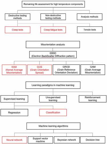
In this study, in order to establish a damage evaluation method using EBSD analysis incorporating that information, and in order to improve the accuracy of damage evaluation for creep and creep-fatigue of heat resistant steels, the following study was performed. Damaged materials were observed using EBSD, which are obtained by interrupted creep tests and interrupted creep-fatigue tests for 304 austenitic stainless steel (JIS SUS304HTB) for boiler tubes use in fossil power plants, and the shapes of crystal grains that can be extracted from KAM maps and GOS (Grain Orientation Spread) maps were approximated with ellipses, after that damage was evaluated by machine learning using these obtained parameters. Figure 1 shows the classification of methods on remaining life assessment for high temperature components (Fujiyama, 2012), methods on misorientation analysis (Fujiyama, 2012), learning paradigms in machine learning (Toshikazu et al., 2017), and machine learning algorithms (Toshikazu et al., 2017). The methods and the algorithms selected in this study are shown in red in Figure 1.

Figure 1. The classification of algorithms and methods in this study

2. Experimental procedures

2.1. Material and specimens

The material for investigation is 304 austenitic stainless steel for boiler tube use in fossil power plants, and the chemical composition and the mechanical properties at ambient temperature are shown in Appendix Tables A1 and A2. The creep test piece was a round bar test piece with a gauge length of 30 mm and a diameter of 6 mm (see Appendix Figure A1). The creep-fatigue test piece was a round bar test piece with a gauge length of 20 mm and a diameter of 8 mm (see Appendix Figure A2). The heat treatment was performed at 1070 °C for 10 minutes and then water-cooled solution treatment.

2.2. Creep tests

Creep tests were conducted with the single lever type creep testing machine made by Toshin Kogyo Co., LTD at the temperature of 650 °C (923 K) and the stress of 130MPa in air. Creep tested specimens were interrupted and observed for the longitudinal cross sections at 0, 10, 20, 50, 80, and 100% of estimated rupture time (Kurashige & Fujiyama, 2019, Harada, 2015).

2.3. Creep-fatigue tests

Creep-fatigue tests were conducted with a 49-kN capacity electro-hydraulic servo-controlled fatigue testing machine coupled with the high frequency induction heating device at the temperature of 650°C (923 K), the total strain range of 1%, the strain rate of 0.1%/sec and tension hold time of 10 min using strain controlled tension hold trapezoidal wave shape (see Appendix Figure A3). The cycles to failure were determined as the number of cycles at 25% drop of peak stress from the steady state of peak stress trend against imposed cycles. Creep-fatigue tested specimens were interrupted and observed for the longitudinal cross sections at 0, 20, 50, and 100% of estimated failure cycles (Kurashige & Fujiyama, 2020, Harada, 2015).

2.4. Misorientation analysis

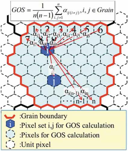
For the misorientation analysis by the EBSD method, KAM maps and GOS maps were made and digitized. Appendix Figure A4 shows the definition of KAM. A hexagon element is counted as one pixel and the distance between two parallel sides is defined as the step size d_s. The numerical KAM value is determined by the average of neighboring six pixels for individual measurement points. Appendix Figure A5 shows the definition of GOS. GOS is the average of the misorientation between the smallest pixel and other pixels in a grain (Kurashige, 2020, Harada, 2015).

3. Damage evaluation method based on grain information by EBSD

3.1. Process of approximating crystal grains by ellipses

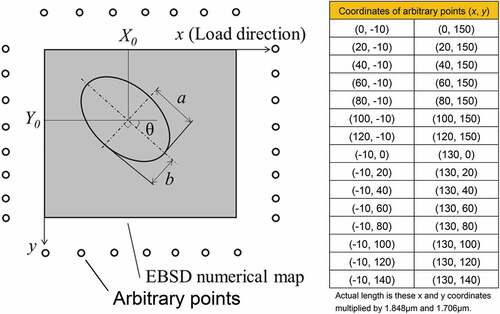
A system for automatically extracting crystal grains and performing elliptic approximation were developed using Python, which is a programming language often used in statistical processing. As a GOS value is unique for each crystal grain, crystal grains can be extracted by extracting pixels with the same GOS value. Data of more than 50 pixels were extracted as crystal grains to eliminate unwanted noise. When the KAM values or the GOS values take 0 or less, they are recognized as noise, and excluded. The number of extracted crystal grains was set up to be 50 per a map, and each crystal grain was extracted randomly. In order to approximate a crystal grain with an ellipse, it is necessary to extract the peripheral coordinates of the crystal grain. Thirty arbitrary points are set around EBSD maps (see Appendix Figure B1), and the system in this study extracts the closest coordinates to each arbitrary point and the maximum coordinates and the minimum coordinates of x and y within crystal grains in xy coordinate system. Moreover, the duplicate data was deleted from those obtained x and y coordinates of 34 points, and crystal grains were approximated with ellipses using those x and y coordinates except duplicate coordinates based on those formulas as shown in Section Section 4.2. The final outputs were the KAM average values of crystal grains, the GOS values of crystal grains, the KAM average values in the closest vicinity of grain boundary, the center coordinates X0 and Y0 of an ellipse, the inclination of the ellipse as θ (degree), the length of x in the x-axis direction as a and the length in the y-axis direction as b (Kurashige, 2020).

3.2. The general formula of elliptic approximation

Equation (1) shows the general formula used for elliptic approximation. The left side of Equation (1) is expanded and rearranged for Xi and Yi, and then Equation (1) becomes Equation (2). Shift 1 from the right side to left side of Equation (2), divide each term by the coefficient of $X_i^2$, and replace the coefficients of each term with the variables A to E. Equation (3) becomes the formula to be replaced with A to E. The values of A to E should be determined so that Equation (4), which is the sum of the squares of the Equation (3), is minimized. Equation (4) can be expressed as a matrix as shown in Equation (5). In order to calculate A to E, it is transformed as shown in Equation (6), and Equation (7) to Equation (11) show finally obtained the formulas for calculating X₀,Y₀,θ, a, and b (Imaging solution, 2019).

(1) ${\left(\frac{\left(X_i-X_0\right)cos\theta +\left(Y_i-Y_0\right)sin\theta }{a}\right)}^2+{\left(\frac{-\left(X_i-X_0\right)sin\theta +\left(Y_i-Y_0\right)cos\theta }{b}\right)}^2=1$(1)

(2) $\begin{array}{rl}& \left(\frac{{cos}^2\theta }{a^2}+\frac{{sin}^2\theta }{b^2}\right)X_i^2+\left(\frac{{sin}^2\theta }{a^2}+\frac{{cos}^2\theta }{b^2}\right)Y_i^2+2\left(\frac{1}{a^2}-\frac{1}{b^2}\right)sin\theta cos\theta X_i{Y}_i\\ & -2\left(\frac{X_0{cos}^2\theta +Y_{0}sin\theta cos\theta }{a^2}+\frac{X_0{sin}^2\theta -Y_{0}sin\theta cos\theta }{b^2}\right)X_i\\ & -2\left(\frac{X_{0}sin\theta cos\theta +Y_0{sin}^2\theta }{a^2}+\frac{Y_0{cos}^2\theta -X_{0}sin\theta cos\theta }{b^2}\right)Y_i\\ & +\frac{X_0^2{cos}^2\theta +2X_0{Y}_{0}sin\theta cos\theta +Y_0^2{sin}^2\theta }{a^2}\\ & +\frac{X_0^2{sin}^2\theta -2X_0{Y}_{0}sin\theta cos\theta +Y_0^2{cos}^2\theta }{b^2}=1\end{array}$(2)

(3) $X_i^2+A{X}_i{Y}_i+B{Y}_i^2+C{X}_i+D{Y}_i+E=0$(3)

(4) $\sum {\left(X_i^2+A{X}_i{Y}_i+B{Y}_i^2+C{X}_i+D{Y}_i+E\right)}^2=0$(4)

(5) $\left(\begin{array}{c}\begin{array}{c}\sum X_i^2{Y}_i^2\begin{array}{cc}\sum X_i{Y}_i^3& \sum X_i^2{Y}_i\begin{array}{cc}\sum X_i{Y}_i^2& \sum X_i{Y}_i\end{array}\end{array}\\ \sum X_i{Y}_i^3\begin{array}{cc}\sum Y^4& \sum Y_i^2\begin{array}{cc}\sum Y^3& \sum Y_i^2\end{array}\end{array}\\ \sum X_i^2{Y}_i\begin{array}{cc}\sum X_i{Y}_i^2& \sum X_i^2\begin{array}{cc}\sum X_i{Y}_i& \sum X_i\end{array}\end{array}\end{array}\\ \begin{array}{c}\sum X_i{Y}_i^2\begin{array}{cc}\sum Y^3& \sum X_i{Y}_i\begin{array}{cc}\sum Y_i^2& \sum Y_i\end{array}\end{array}\\ \sum X_i{Y}_i\begin{array}{cc}\sum Y_i^2& \sum X_i\begin{array}{cc}\sum Y_i& \sum 1\end{array}\end{array}\end{array}\end{array}\right)\left(\begin{array}{c}A\\ B\\ C\\ D\\ E\end{array}\right)=\left(\begin{array}{c}-\sum X_i^3{Y}_i\\ -\sum X_i^2{Y}_i^2\\ -\sum X_i^3\\ -\sum X_i^2{Y}_i\\ -\sum X_i^2\end{array}\right)$(5)

(6) $\left(\begin{array}{c}A\\ B\\ C\\ D\\ E\end{array}\right)=\left(\begin{array}{c}\begin{array}{c}\sum X_i^2{Y}_i^2\begin{array}{cc}\sum X_i{Y}_i^3& \sum X_i^2{Y}_i\begin{array}{cc}\sum X_i{Y}_i^2& \sum X_i{Y}_i\end{array}\end{array}\\ \sum X_i{Y}_i^3\begin{array}{cc}\sum Y^4& \sum Y_i^2\begin{array}{cc}\sum Y^3& \sum Y_i^2\end{array}\end{array}\\ \sum X_i^2{Y}_i\begin{array}{cc}\sum X_i{Y}_i^2& \sum X_i^2\begin{array}{cc}\sum X_i{Y}_i& \sum X_i\end{array}\end{array}\end{array}\\ \begin{array}{c}\sum X_i{Y}_i^2\begin{array}{cc}\sum Y^3& \sum X_i{Y}_i\begin{array}{cc}\sum Y_i^2& \sum Y_i\end{array}\end{array}\\ \sum X_i{Y}_i\begin{array}{cc}\sum Y_i^2& \sum X_i\begin{array}{cc}\sum Y_i& \sum 1\end{array}\end{array}\end{array}\end{array}\right)\left(\begin{array}{c}-\sum X_i^3{Y}_i\\ -\sum X_i^2{Y}_i^2\\ -\sum X_i^3\\ -\sum X_i^2{Y}_i\\ -\sum X_i^2\end{array}\right)$(6)

(7) $X_0=\frac{AD-2BC}{4B-A^2}$(7)

(8) $Y_0=\frac{AC-2D}{4B-A^2}$(8)

(9) $\theta =\frac{{tan}^{-1}\left(\frac{A}{1-B}\right)}{2}$(9)

(10) $a=\sqrt{{\left(X_{0}cos\theta +Y_{0}sin\theta \right)}^2-E{cos}^2\theta -\left\{{\left(X_{0}sin\theta -Y_{0}cos\theta \right)}^2-E{sin}^2\theta \right\}\frac{{sin}^2\theta -B{cos}^2\theta }{{cos}^2\theta -B{sin}^2\theta }}$(10)

(11) $b=\sqrt{{\left(X_{0}sin\theta -Y_{0}cos\theta \right)}^2-E{sin}^2\theta -\left\{{\left(X_{0}cos\theta +Y_{0}sin\theta \right)}^2-E{cos}^2\theta \right\}\frac{{cos}^2\theta -B{sin}^2\theta }{{sin}^2\theta -B{cos}^2\theta }}$(11)

where $X_0$ and $Y_0$ are the center coordinates of ellipses, $X_i$ and $Y_i$ are the coordinates on the circumference of the ellipse, $\theta$ is a slope of ellipses, $a$ is a length in the X-axis direction, $b$ is a length in the Y-axis direction, A to E are constants.

3.3. Construction of a neural network

In this study, a neural network which demonstrates high classification accuracy of pattern recognition is used. The configuration of the neural network used in this study is shown below. The speed of learning was increased and over-fitting was suppressed by normalizing to mean 0 and variance 0 using Batch Normalization (Santurkar et al., 2018). ReLU (Rectified Linear Unit; Hara et al., 2015) shown in Equation (12) was used for the activation function of the hidden layers, and the Softmax function shown in Equation (13) was used for the activation function of the output layer. Cross entropy (Pieter-Tjerk De et al., 2005) as shown in Equation (14) was used for the loss function. In this study, backpropagation (Werbos, 1990) is adopted as a method of calculation from the output layer to input layer using a theorem called the chain rule. Figure 2 shows a simplified model of the neural network used in this study. It has three intermediate layers, and the structures of the intermediate layers and the output layer are shown in Figure 2. N1–N3 in Figure 2 show the number of nodes at the first to third layers of the intermediate layers. N1, N2, and N3 were set up 20 to 100, 15 to 95, and 10 to 90. The nodes were optimized by always kept N1 > N2 > N3 changed the number of nodes every 5 nodes using the round robin. The default of the number of nodes were determined as N1 = 100, N2 = 90, and N3 = 80. Adam that is an algorithm that fuses Momentum and AdaGrad was used to optimize the parameters. Equations (15)–(20) show Adam’s update formula (Diederik & Ba, 2015). In this study, these a and ε as the learning rates are set up 0.001 and 10⁻⁸. Those algorithms were implemented using Python of the programming language, and learning and evaluation were performed.

(12) $f\left(x\right)=max\left(0,x\right)$(12)

(13) $y_k=\frac{exp\left(a_k\right)}{{\sum }_{i=1}^n\mathrm{e}\mathrm{x}\mathrm{p}\left(a_i\right)}$(13)

(14) $E=-\sum _k{t}_{k}log{y}_k$(14)

(15) $g_t={\mathrm{\nabla }}_{\theta }{f}_t({\theta }_{t-1})$(15)

(16) $m_t={\beta }_1{m}_{t-1}+\left(1-{\beta }_1\right)g_t$(16)

(17) $v_t={\beta }_2{v}_{t-1}+\left(1-{\beta }_2\right){g_t}^2$(17)

(18) $\widehat{m_t}=\frac{m_t}{\left(1-{\beta }_1^t\right)}$(18)

(19) $\widehat{v_t}=\frac{v_t}{\left(1-{\beta }_2^t\right)}$(19)

(20) ${\theta }_{t+1}={\theta }_t-\alpha \frac{\stackrel{\wedge }{m_t}}{\sqrt{\stackrel{\wedge }{v_t}}+\epsilon }$(20)

where $x$ is an input value for ReLU in intermediate layers, $a_k$ and $a_i$ are kth and ith input values for the Softmax function, $y_k$ is an output value of the Softmax function as well as an input value of the cross entropy, $n$ is the number of output layers, $t_k$ is a correct answer label, $E$ is an output value of the cross entropy, $f$ is stochastic objective function, $\theta$ is update parameters, $g$ is a gradient, suffix $t$ is a timestep, ${\beta }_1$ and ${\beta }_2$ are exponential decay rates for the moment estimates, ${\beta }_1^t$ and ${\beta }_2^t$ show ${\beta }_1$ and ${\beta }_2$ to the power of $t$, $m$ is a 1^st moment vector, $v$ is 2^nd moment vector, $\alpha$ is a stepsize, $\epsilon$ is coefficient to prevent division by zero (Diederik & Ba, 2015).

Figure 2. Schematic model of neural network

3.4. Data sets

The explanatory variables used in this analysis are KAM average, GOS, areas of crystal grains, KAM average near the grain boundary, absolute value of ellipse angle to load axis, and the minor axis/the major axis (aspect ratio). The objective variable used in this analysis is damage rates. The number of EBSD images obtained from the creep test materials was three for each damage rate, and there were 150 crystal grain data for each damage rate because 50 crystal grains were extracted for each map. These data were divided into 120 learning data and 30 evaluation data. Besides, the analysis was performed using the relative frequency of KAM obtained for each crystal grain. The learnings were performed at the following rank of KAM: 10, 20, 25, 40, 50, 80, 100, 125, 160, 200, 250, 400, 500, 625, 800, 1000, 1600, 2500, 3200, and 4000. In addition, ensemble learnings were performed using these obtained 20 results. Ensemble learning is the method of training multiple learners individually and averaging the obtained output. It is known that recognition accuracy is improved by using this method (Sagi & Rokach, 2018). The number of EBSD images obtained from the creep-fatigue test samples was two for each damage rate, and as 50 crystal grains were extracted from each map, there were 100 crystal grain data for each damage rate. These data were divided into 70 learning data and 30 evaluation data. The learning method and data for creep and creep-fatigue are summarized in Appendix Table B1 (Kurashige, 2020).

4. Results and discussion on damage evaluation based on grain information of EBSD for creep

4.1. Damage evaluation based on grain information of EBSD for creep

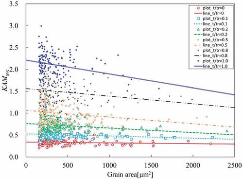
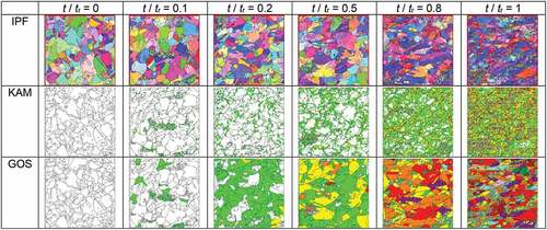
Part of the EBSD maps obtained for Creep damage materials is shown in Appendix Figure C1. Figure 3 to Figure 6 show the relationships between the damage rates and KAM average, grain areas [μm²] (Kurashige, 2020), absolute value of angle from tensile axis, or aspect ratio of the ellipses. The plots shown in Figure 3 to Figure 6 are actual data, and the straight line are drawn by linear interpolations between each damage rate. It can be seen that KAM average on grain boundary is larger than KAM average as shown in Figure 3. This means that as the damage progress, dislocations accumulate adjacent to the crystal grains. It can be seen that the dispersion of the data increases as the damage rate increases. From these facts, it is considered that there are two types of crystal grains with and without grain boundary piling up dislocations. From Figure 4, it can be seen that the crystal grain areas are almost unchanged for the damage rate of 0–0.8; however, the crystal grain areas are decreasing for the damage rate of 0.8–1. It is thought that recrystallization occurred after the damage rate of 0.8, and many small crystals were formed, therefore the grain areas were reduced. It can be seen from Figure 5 that the angle to the tensile axis decreases as the damage rate increases. It is found from Figure 6 that the aspect ratio slightly tends to decrease as the damage rate increases. The tendency of each measured quantity was investigated for each crystal grain at each damage rate, owing to the large variations of data in each damage rate, as shown in Figures 3 to 6. Figure 7 shows the relationship between the KAM average and the crystal grain areas for each crystal grain at each damage rate. It can be seen from this graph that the KAM average decreases as the crystal grain areas increase at any damage rate. In addition, it found that the larger the damage rate, the stronger that tendency. Moreover, this graph shows that the smaller the crystal grain areas, the larger the KAM average, because the smaller the crystal grain areas, the larger the proportion of the crystal grain areas close to the grain boundary.

Figure 3. Relationship between KAM_ave and t/t_r.

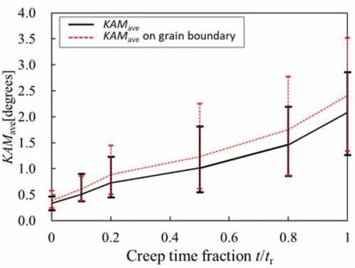
Figure 4. Relationship between grain area and t/t_r.

Figure 5. Relationship between angle from pulling direction and t/t_r.

Figure 6. Relationship between (half of the minor axis)/(half of the major axis) and t/t_r.

Figure 7. Relationship between KAM_ave and grain area

4.2. Machine learning using grain information of EBSD for creep test

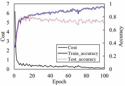
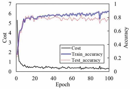
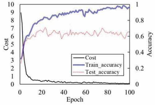
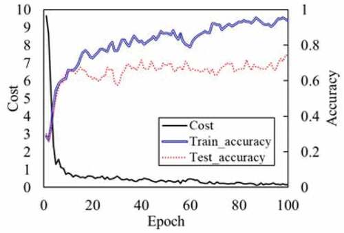
The learning and evaluation were performed with the neural network using the explanatory variables of KAM average, GOS, grain areas, KAM average on grain boundary, absolute value of ellipse angle to load axis, and ellipse aspect ratio, and using the objective variable of damage rates. As the learning progress, the cost decreases and the classification accuracy of the learning data increases; however, since the classification accuracy of the evaluation data is decreasing, it can be seen that overfitting to learning data occurred (see Appendix Figures C2 and C3). Figure 8 shows the classification accuracy using default nodes and optimized nodes. It can be seen from Figure 8 that the classification accuracy was improved in the damage rates of 0.1 to 0.8 by using optimized nodes. The predicted damage rates by neural network and the damage rates of the actual evaluation data are shown in Appendix Tables C1 and C2 as the confusion matrix.

Figure 8. Relationship between accuracy and creep time fraction t/t_r.

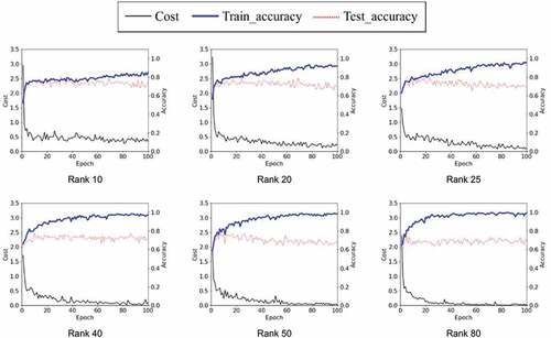
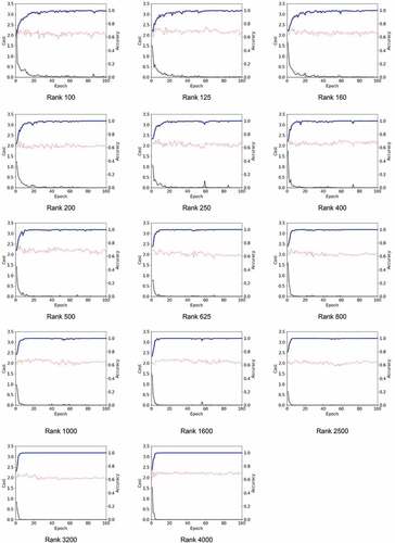
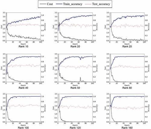
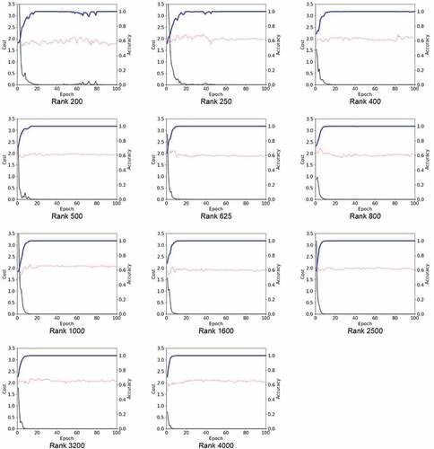
In the next, the learning results using the relative frequency of KAM obtained from crystal grains are described. It can be seen that the accuracies for the evaluation data deviate from the accuracies for the learning data as the ranks of KAM increase (see Appendix Figure C4). In other words, if the rank of KAM is too large, the classification accuracy for the learning data is increased, but the classification accuracy for the evaluation data is decreased because overfitting is occurred. Figure 9 shows the classification accuracy using default nodes, the classification accuracy using optimized nodes and their difference. It can be seen from Figure 9 that the classification accuracy slightly decreases as the number of classes increases. The classification accuracy using a single rank is 0.7844 at the maximum, but the classification accuracy is improved to 0.9833 by ensemble learning using optimized nodes. This result shows that ensemble learning is a powerful preventative measure against overfitting. Figure 10 shows that how the classification accuracy changes in the event that the number of learners is changed in ensemble learning. The number of learners is increased randomly, as shown in Appendix Table C3. As a result, it is found that the classification accuracy is improves as the number of learners increases. It can be seen that the accuracy is greatly improved when the number of learners is increased from 2 to 6, and the classification accuracy is slightly increased when the number of learners is increased from 10 to 20. From this fact, it is considered that the classification accuracy improves rapidly as the number of learners increases, and becomes saturated after that. Figure 11 and Appendix Tables C4 and C5 show the classification results and the classification accuracy when ensemble learning is performed with 20 learners using the optimized nodes and the default nodes. It can be seen from these tables and graphs, the classification accuracy by ensemble learning using default nodes is 0.9556, and using optimized nodes is 0.9833. The number of misclassifications using optimized nodes was 3, and the classification accuracy was 1.0 except for the evaluation data with a damage rate of 0.5. The classification accuracy was able to greatly improve compared with the classification accuracy shown in Figure 8 and Appendix Tables C1 and C2.

Figure 9. Accuracy of default node, optimized and their difference at each rank and ensemble

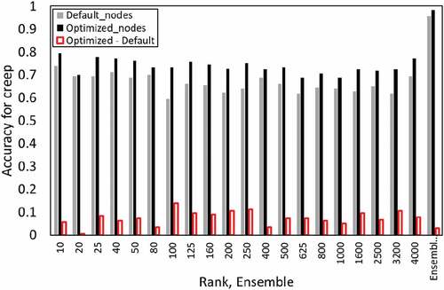
Figure 10. Relationship between number of ensemble learners and accuracy for the combination shown in Appendix Table C3

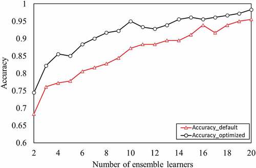
Figure 11. Relationship between accuracy and creep time fraction t/t_r by ensemble learning

5. Results and consideration of damage evaluation based on grain information of EBSD for creep-fatigue

5.1. Damage evaluation based on grain information of EBSD for creep-fatigue

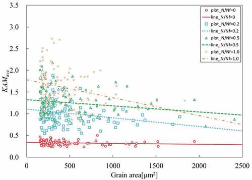
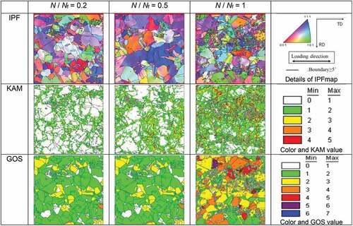
Part of the EBSD maps obtained for Creep-fatigue damage materials is shown in Appendix Figure D1. Figures 12 to 16 show figure of the same format as Figures 3 to 7, respectively. It can be seen from Figure 12 that KAM average adjacent to the grain boundaries and the variation of that are higher than KAM average in crystal grains and the variation of that. This tendency is the same as that tendency shown in Figure 3. From Figure 13, it can be seen that the crystal grain areas increase up to the damage rate of 0.5, and then, the crystal grain areas decrease. This tendency is different from that tendency shown in Figure 4. It can be seen from Figure 14 that the angle from loading direction decreases as the damage rate increases. Figure 15 shows relationship between (half of the minor axis)/(half of the major axis) and N/N_f. Figure 16 shows the relationship between grain areas and KAM average for each grain at each damage rate. Although the variation is extremely large, the larger crystal grain areas, the smaller KAM average for each crystal grain at all damage rates.

Figure 12. Relationship between KAM_ave and N/N_f.

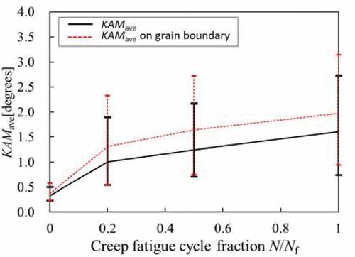
Figure 13. Relationship between grain area and N/N_f.

Figure 14. Relationship between angle from loading direction and N/N_f.

Figure 15. Relationship between (half of the minor axis)/(half of the major axis) and N/N_f.

Figure 16. Relationship between KAM_ave and grain area

5.2. Machine learning using grain information of EBSD for creep-fatigue test

The learning and evaluation were performed with the neural network using the explanatory variables of KAM average, GOS, grain areas, KAM average on grain boundary, absolute value of ellipse angle to load axis, and ellipse aspect ratio, and using the objective variable of damage rates. Overfitting occurred as with the neural network using EBSD information of creep damaged materials (see Appendix Figures D2 and D3). Figure 17 shows the classification accuracy as a bar graph. It can be seen from Figure 17 that as a result of optimizing the nodes, the classification accuracy is improved at the damage rates of 0.5 and 1. Appendix Tables D1 and D2 show the confusion matrix.

Figure 17. Relationship between accuracy and creep fatigue cycle fraction N/N_f.

In the next, the learning results using the relative frequency of KAM obtained from crystal grains are described. The classification accuracy of the learning data has large deviation from the classification accuracy of the evaluation data as with creep damaged materials (see Appendix Figure D4). It is necessary to take measures such as reducing the number of layers of the neural network, increasing the number of training data and introducing algorithms such as weight decay to prevent overfitting. Figure 18 shows the classification accuracy using default nodes, the classification accuracy using optimized nodes and their difference. The classification accuracy using a single rank is 0.7250 at the maximum, but the classification accuracy is improved to 0.9750 by ensemble learning using optimized nodes. As in the case of creep damage materials, overfitting could be suppressed by ensemble learning. Ensemble learning was able to improve the evaluation accuracy of creep damaged materials and creep-fatigue damaged materials. Figure 19 shows that how the classification accuracy changes when the number of learners is changed in ensemble learning. The number of learners is increased as shown in Appendix Table C3. As a result, it is found that the classification accuracy of the evaluation data improves as the number of learners increases. Figure 20 and Appendix Tables D3 and D4 show the classification results and the accuracy when ensemble learning is performed with 20 learners using the nodes before optimization and after optimization. It can be seen from these tables and graphs, the classification accuracy by ensemble learning using default nodes is 0.8083, and using optimized nodes is 0.9750. The classification accuracy for creep damaged materials using the optimized nodes was not so high compared with the classification accuracy using the default nodes as shown in Figure 11. However, the classification accuracy for creep-fatigue damaged materials using the optimized nodes was significantly increased compared with the classification accuracy using default nodes, as shown in Figure 20.

Figure 18. Accuracy of default node, optimized and their difference at each rank and ensemble

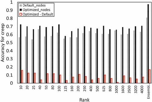
Figure 19. Relationship between number of ensemble learners and accuracy for the combination shown in Appendix Table C3

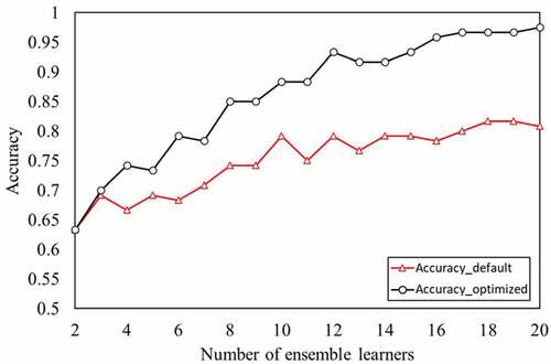
Figure 20. Relationship between accuracy and creep fatigue cycle fraction N/N_f by ensemble learning

6. Conclusions

EBSD observations were performed for the damaged materials obtained by the creep and the creep-fatigue interrupted tests for 304 austenitic stainless steel for boiler tube use in fossil power plants. As a result, it was quantitatively found that as the damage progress due to creep and creep-fatigue, the crystal grains expand in the loading direction. Furthermore, it became clear that the larger the areas of the crystal grains, the smaller the KAM average of the crystal grains. The damage evaluation system using the neural network has been developed using the parameters obtained by ellipse approximation of the crystal grains obtained from EBSD images. As a result, ensemble learning showed the best classification accuracy using the 20 learners obtained by changing the rank of the relative frequency of KAM. It was found that the classification accuracy improves as the number of learners for ensemble learning increases. It was proved to be able to estimate the damage rates with the classification accuracy of 98.33% for creep test materials and 97.50% for creep-fatigue test materials using the information from one of crystal grains in the EBSD image. Therefore, the system developed in this study is effective for detailed evaluation including the size and the shape of crystal grains obtained by EBSD observations for creep damage and creep-fatigue damage for 304 austenitic stainless steel.

Acknowledgements

The authors are grateful to thank the members of the Fujiyama Laboratory of Meijo University for accumulating data of the material tests and EBSD observations used in this study.

Disclosure statement

No potential conflict of interest was reported by the author(s).

Additional information

Funding

The authors received no direct funding for this research.

Notes on contributors

Yu Kurashige

Yu Kurashige has conducted research to apply machine learning to damage evaluation for high temperature materials, and each process of this research was conducted by the following persons. The conception and study design were made by Yu Kurashige and Kazunari Fujiyama. The evaluation system was to construct by Yu Kurashige and Sho Takami. Processing and analysis of experimental data were conducted by Yu Kurashige and Sho Takami. The discussion of the research results was carried out by Yu Kurashige and Kazunari Fujiyama. This paper was written by Yu Kurashige, and reviewed by Kazunari Fujiyama and Sho Takami.

Appendix

A) Experimental conditions

Table A1. Chemical composition of SUS304HTB (mass %)

C	Si	Mn	P	S	Cr	Mo	Ni	V	Cu	N
0.06	0.53	1.45	0.025	0.012	18.38	0.22	10.04	<0.01	0.12	0.029

Table A2. Tensile properties at ambient temperature

0.2% proof stress (MPa)	Tensile strength (Mpa)	Elongation (%)
253	594	61

Figure A1. Creep test specimen and sampling portion.

Figure A2. Creep-fatigue test specimen and sampling portion.

Figure A3. Trapezoidal wave of tensile holding by strain control.

Figure A4. Definition of KAM within a grain.

Figure A5. Definition of GOS within a grain.

B)

Damage evaluation methods

Figure B1. Schematic view of EBSD numerical map and elliptic approximation parameters.

Table

Coordinates of arbitrary points (x, y)
(0, −10)	(0, 150)
(20, −10)	(20, 150)
(40, −10)	(40, 150)
(60, −10)	(60, 150)
(80, −10)	(80, 150)
(100, −10)	(100, 150)
(120, −10)	(120, 150)
(−10, 0)	(130, 0)
(−10, 20)	(130, 20)
(−10, 40)	(130, 40)
(−10, 60)	(130, 60)
(−10, 80)	(130, 80)
(−10, 100)	(130, 100)
(−10, 120)	(130, 120)
(−10, 140)	(130, 140)
Actual length is these x and y coordinates multiplied by 1.848μm and 1.706μm.

Table B1. Learning methods and data for creep and creep fatigue

	Creep	Creep-fatigue
Explanatory variables	KAMave,GOS,Grain area, KAMave on grain boundary, (Minor axis length of ellipse) / (Major axis length of ellipse), Angle from load axis	Same as creep
Explanatory variables for ensemble learning	Relative frequency of KAM Rank as 10, 20, 25, 40, 50, 80, 100, 125, 160, 200, 250, 400, 500, 625, 800, 1000, 1600, 2500, 3200, 4000	Same as creep
Objective variable	Creep time fraction t / tr t / tr = 0, 0.1, 0.2, 0.5, 0.8, 1	Creep-fatigue cycle fraction N / Nf = 0, 0.2, 0.5, 1
Number of data of a map	50	50
Number of Observation place	3	2
Number of data at each damage rate	150	100
Number of training data at each damage rate	120	70
Number of evaluation data at each damage rate	30	30
Total number of data	900	400
Activation function of Intermediate layer	ReLU (Rectified Linear Unit)	Same as creep
Activation function of Output layer	Softmax	Same as creep
Loss function	Cross entropy	Same as creep
Optimization for parameter update	Adam	Same as creep
Number of nodes in input layer	6 or Rank of Relative frequency of KAM	Same as creep
Number of nodes in intermediate layer	Default as 100, 90, 80 Optimized to the values shown in the Table 6	Same as creep
Number of nodes in output layer	6	4

C)

Results for creep

Figure C1. EBSD maps for Creep damage materials.

Figure C2. Relationship between cost and epoch, accuracy and epoch for (N1, N2 N3) = (100, 90.

Figure C3. Relationship between cost and epoch, accuracy and epoch for (N1, N2, N3) = (45, 30, 10) as optimal number of nodes.

Table C1. Confusion matrix for (N1, N2 N3) = (100, 90, 80)

Table C2. Confusion matrix for (N1, N2, N3) = (45, 30, 10) as optimal number of nodes

Figure C4. Relationship between cost and epoch, accuracy and epoch for each rank.

Table C3. Pattern of ensemble learner combination pattern

Table C4. Confusion matrix for (N1, N2 N3) = (100, 90, 80) by ensemble learning

Table C5. Confusion matrix at optimal number of nodes by ensemble learning

D)

Results for creep-fatigue

Figure D1. EBSD maps for creep-fatigue damage materials.

Figure D2. Relationship between cost and epoch, accuracy and epoch for (N1, N2 N3) = (100, 90, 80).

Figure D3. Relationship between cost and epoch, accuracy and epoch for (N1, N2, N3) = (100, 35, 25) as optimal number of nodes.

Figure D4. Relationship between cost and epoch, accuracy and epoch for each rank.

Table D1. Confusion matrix for (N1, N2 N3) = (100, 90, 80)

Table D2. Confusion matrix for (N1, N2, N3) = (100, 35, 25) as optimal number of nodes

Table D3. Confusion matrix for (N1, N2 N3) = (100, 90, 80) by ensemble learning

Table D4. Confusion matrix at optimal number of nodes by ensemble learning

References

- Diederik, P., & Ba, J. L. (2015). Adam: Amethod for stochastic optimization, In The 3rd international conference on learning representations (ICLR), San Diego (pp. 1–15). https://arxiv.org/abs/1412.6980v9
- Fujiyama, K. (2012). The Frontier of Technology Development in Remaining Life Assessment for High Temperature Components. Journal of the Society of Materials Science, Japan, 61(11), 919–36. https://doi.org/10.2472/jsms.61.919
- Fujiyama, K., & Harada, K. (2015). Akihiro Ogawa and Hirohisa Kimachi, “EBSD Analysis of Grain Strain Distribution for Creep Damaged SUS304HTB. Journal of the Society of Materials Science, Japan, 64(2), 88–93. https://doi.org/10.2472/jsms.64.88
- Fujiyama, K., Mizutani, Y., Taniguchi, Y., & Kimachi, H. (2013). EBSD Analysis of Creep Damage Process in SUS304HTB Steel. Journal of the Society of Materials Science, Japan, 62(5), 305–310. https://doi.org/10.2472/jsms.62.305
- Fujiyama, K., Ogawa, A., Harada, K., & Kimachi, H. (2015). EBSD Analysis of Grain Strain Distribution for Creep Damaged Modified 9Cr Steel. Journal of the Society of Materials Science, Japan, 64(2), 94–99. https://doi.org/10.2472/jsms.64.94
- Fukuda, M. (2014). Advanced USC Technology Development. Journal of Smart Processing, 3(2), 78–85. https://doi.org/10.7791/jspmee.3.78
- Hara, K., Saito, D., & Shouno, H., “Analysis of Function of Rectified Linear Unit Used in Deep Learning”, 2015 International Joint Conference on Neural Networks (IJCNN 2015), Killarney. https://doi.org/10.1109/IJCNN.2015.7280578
- Harada, K., “Evaluation of grain strain distribution in creep and creep-fatigue damaged SUS304HTB steel through EBSD observation”, Master Thesis (2015), Meijo University.
- Imaging solution, available from https://imagingsolution.blog.fc2.com/blog-entry-20.html, (10 December, 2019).
- Kurashige, Y., “Investigation on the applicability of machine learning and statistical analysis of creep and creep-fatigue damage evaluation for heat resistant steel”, Master Thesis (2020), Meijo University.
- Kurashige, Y., & Fujiyama, K. (2019). Development of creep damage AI evaluation system for austenitic stainless steel. Transactions of the Japan Society of Mechanical Engineers (In Japanese), 85(878), 1–9. https://doi.org/10.1299/transjsme.18-00436
- Kurashige, Y., & Fujiyama, K. (2020). Application of Machine Learning and Statistical Analysis to Creep and Creep-Fatigue Damage Evaluation for Austenitic Stainless Steel. Journal of the Society of Materials Science, Japan, 69(9), 666–671. https://doi.org/10.2472/jsms.69.666
- Kuroda, M., Kamaya, M., Mori, T., & Izaki, T. (2013). Detection of Fatigue Damage in Stainless Steel by EBSD Analysis (Analysis Focused on Grain Boundaries). Transactions of the Japan Society of Mechanical Engineers, Series A, 79(807), 1690–1694. https://doi.org/10.1299/kikaia.79.1690
- Nakamura, T., Kataoka, O., Yoshimura, H., Hirata, H., & Fujiyama, K. (2021). EBSD Evaluation of Creep Damage Process for Fine Grained Heat Affected Zone of Serviced Mod.9Cr-1Mo Steel. Journal of the Society of Materials Science, Japan, 70(2), 169–176. https://doi.org/10.2472/jsms.70.169
- Nomura, K., Kubushiro, K., Sakakibara, Y., Takahashi, S., & Yoshizawa, H. (2012). Effect of Grain Size on Plastic Strain Analysis by EBSD for Austenitic Stainless Steels with Tensile Strain at 650°C. Journal of the Society of Materials Science, Japan, 61(4), 371–376. https://doi.org/10.2472/jsms.61.371
- Nomura, Y., & Shigemura, K. (2019). Development of Real-Time Screening System for Structural Surface Damage Using Object Detection and Generative Model Based on Deep Learning. Journal of the Society of Materials Science, Japan, 68(3), 250–257. https://doi.org/10.2472/jsms.68.250
- Ogata, T. (2012). Damage Evaluation Method for High-Temperature Components in Thermal Power Plants. Transactions of the Japan Society of Mechanical Engineers, Series A, 78(789), 694–707. https://doi.org/10.1299/kikaia.78.694
- Oinuma, S., Takaku, R., Nakatani, Y., & Takeyama, M. (2021). Effect of Microstructure and Deformation on Hardness Distribution of Wrought Precipitation Strengthened Ni-Based Alloy after Creep Damage. Journal of the Society of Materials Science, Japan, 70(3), 258–263. https://doi.org/10.2472/jsms.70.258
- Pieter-Tjerk De, B., Kroese, D. P., Mannor, S., & Rubinstein, R. Y. (2005). A Tutorial on the Cross-Entropy Method. In Manufactured in The Netherlands, Annals of Operations Research (Vol. 134, 2005, pp. 19–67). Springer Science + Business Media, Inc. https://doi.org/10.1007/s10479-005-5724-z
- Pouyanfar, S., Sadiq, S., Yan, Y., Tian, H., Tao, Y., Reyes, M. P., Shyu, M.-L., Chen, S.-C., & Iyengar, S. S. (2018). A survey on deep learning: Algorithms, techniques, and applications. ACM Computing Surveys, 51(5), 1–36. https://doi.org/10.1145/3234150.
- Sagi, O., & Rokach, L. (2018). Ensemble learning: A survey. WIREs Data Mining and Knowledge Discovery, 8(4), 1–18. https://doi.org/10.1002/widm.1249
- Santurkar, S., Tsipras, D., Ilyas, A., & Madry, A. (2018). How does batch normalization help optimization? In The 32nd conference on Neural Information Processing System (NeurIPS 2018), Montreal. https://arxiv.org/abs/1805.11604v5
- Shigemura, K., & Nomura, Y. (2020). A Two-Step Screening System for Surface Crack Using Object Detection and Recognition Technique Based on Deep Learning. Journal of the Society of Materials Science, Japan, 69(3), 218–225. https://doi.org/10.2472/jsms.69.218
- Toshikazu, F., Ryohei, F., Daisuke, O., & Masashi, S. (2017). Outlook for big data and machine learning. Journal of Information Processing and Management, 60(8), 543–554. https://doi.org/10.1241/johokanri.60.543
- Werbos, P. J. (1990). Backpropagation Through Time: What It Does and How to Do It. Proceedings of the IEEE, 78(10), 1550–1560. https://doi.org/10.1109/5.58337
- Yoda, R., Kamaya, M., Kimura, H., Ohtani, T., & Fujiyama, K. (2017). Round Robin Test Using EBSD for Creep Damage Evaluation. Journal of the Society of Materials Science, Japan, 66(2), 130–137. https://doi.org/10.2472/jsms.66.130
- Zhang, S., & Fukutomi, H. (2021). Creep Rupture Behavior for Welded Pipe of Ni-Based Alloy Using Full Thickness Specimen and Application of Nondestructive Damage Detection. Journal of the Society of Materials Science, Japan, 70(2), 184–190. https://doi.org/10.2472/jsms.70.184