Methodology for automatic fault detection in photovoltaic arrays from artificial neural networks

Abstract

This article presents a methodology for automatic fault detection in photovoltaic arrays. Due to the great importance in the construction of increasingly robust photovoltaic plants, automatic fault detection has become a necessary tool to extend the useful life of these plants, avoid system shutdowns and reduce serious safety problems. In the present study, nine possible faults are detected, caused by malfunction in the bypass and blocking diodes. The solution consists of training two models based on artificial neural networks, the first model is a binary classifier that detects whether or not a fault occurs, the second is a multiclass classifier that detects the fault type. The obtained models were trained from simulation data, in an architecture of 9 photovoltaic panels interconnected in three rows by three columns matrix (extendable to larger systems). The evaluation shows that the prediction system has a total accuracy of 92.95%. Finally, this methodology is intended to be implemented in Colombia, in zones with difficult access and not interconnected to the electricity grid, seeking to reduce corrective maintenance.

Keywords:

• Photovoltaic system
• fault detection
• Artificial Neural Network (ANN)
• classification
• sustainable development goals (SDG).

PUBLIC INTEREST STATEMENT

This work presents a methodology for automatic fault detection in photovoltaic arrays, which is intended to be implemented in Colombia, in zones with difficult access and not interconnected to the national electricity grid, NIZ - Non-Interconnected Zones, seeking to reduce corrective maintenance . The obtained models were trained from simulation data, in an architecture of 9 photovoltaic panels interconnected in three rows by three columns matrix (extendable to larger systems). The evaluation shows that the prediction system has a total accuracy of 92.95%.

1. Introduction

Automatic fault detection in photovoltaic (PV) systems has acquired great relevance worldwide, as expressed by (Pierdicca et al., 2018), (Rao et al., 2019), and (Lu et al., 2019). This is due to the necessity of keeping this type of system functioning properly for as long as possible. The early detection of faults in solar plants can be summarized in the reduction of serious safety problems, shutdown of the system and need for corrective maintenance. This will be reflected in the decrease in operating costs.

Moreover, a great deal of work, carried out by different researchers, shows the viability and importance of solving this issue (Dhimish et al., 2018), (Harrou et al., 2018) and (De Benedetti et al., 2018).

Renewable energy sources, such as solar and wind, are promising alternatives to conventional fossil fuels as they are clean, sustainable, safe, environmentally friendly, and with zero CO₂ emissions (Harrou et al., 2018). For example, (Hosenuzzaman et al., 2015) estimates that photovoltaic energy generation will reduce CO₂ emissions by approximately 69 to 100 million tons by 2030.

Additionally, Renewable Energy Technologies (RETs) especially Solar Photovoltaics have seen many plants being constructed to either supplement the grid or as alternatives for those off-grid as argued in (Kibaara et al., 2020). On the other hand, according to (De Benedetti et al., 2018) the reduction in PV system costs, the market price trends, along with the increase in yields from cell efficiency improvements and less electrical conversion losses, has led to a rise in interest in said alternatives for energy production systems.

An example of this is that the photovoltaic industries have recognized important developments in the manufacture of PV equipment as well as the number of facilities (Madeti & Singh, 2018), where the reported installed global PV capacity was 310 GW by late 2016. Therefore, given the advantages posed by PV systems, their use has grown exponentially in the last century. Because of this, as presented by (De Benedetti et al., 2018), issues related to maintenance of PV systems are drawing significant attention in the research field. This is shown by studies and efforts undertaken by several institutions and companies whose objective is to develop “better practices” for PV system operation.

Now, since PV generators (or solar panels) are installed outdoors, as shown by (Madeti & Singh, 2018), continuous exposure to adverse weather conditions (sunlight, rain, etc.) can significantly affect the system’s performance by diminishing its efficiency. In fact, (Harrou et al., 2018) confirms that PV systems are frequently exposed to different fault sources affecting the generated power, including short-circuit, open-circuit and shading faults. These can considerably reduce both the system’s efficiency and its useful life. For instance, a PV system monitoring study was presented by (Firth et al., 2010), where a loss of annual energy of 18.9%, due to several faults, was reported.

In addition to energy losses, faults in PV systems can cause shutdowns, or even severe safety problems. Such is the case presented in (Chen et al., 2019), where two PV installations in United States, a 383 KWp photovoltaic matrix in Bakersfield, CA, and a 1.208 MWp energy plant in Mount Holly, NC, caught fire in 2009 and 2011 respectively. The source of these accidents was a failure in the DC side that was not identified earlier. As such, detecting and identifying faults, as early as possible, in PV systems is key, as (Harrou et al., 2018) outlines.

Now, failures in photovoltaic systems are due to different circumstances, among the most common are failures due to degradation factors of PV modules or electrical failures in the system. Some of the degradation factors of photovoltaic modules are Dirt on the Surface, Optical Degradation, Increase in Series Resistance, Decrease in Parallel Resistance and Degradation of the Anti-reflective Layer.

On the other hand, electrical failures in the photovoltaic system refer to the interconnection of several panels or photovoltaic modules in a matrix manner, this interconnection requires the inclusion of semiconductor devices (bypass diodes and blocking diodes) for the correct operation of each of the panels. Due to this, different faults can occur and are listed in (Madeti & Singh, 2018), such as line-line faults, open-circuit faults, short circuit in the bypass diodes, open circuit in the bypass diodes, open circuit in the blocking diodes and short circuit in the blocking diodes.

Therefore, in the present study only the failures in the by-pass and blocking diodes are taken into account. (Solórzano & Egido, 2014) show, in a solar panel matrix interconnection it is imperative to use bypass and blocking diodes to avoid module hot spots, which can negatively affect the panel’s performance. These diodes prevent modules from absorbing power instead of delivering it when there is shade or dirt. Figure 1 shows a two-row PV matrix with its respective bypass and blocking diodes.

Figure 1. Bypass and blocking diodes

Source: Authors’ own

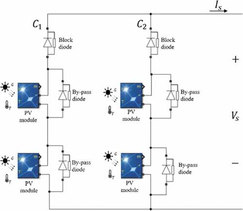
Thus, if any of those diodes breaks, the PV plant performance will be directly affected. The objective of this research is to present a novel method for the extraction and transformation of information for the creation of a mathematical model capable of detecting operating problems in bypass and blocking diodes.

2. Literature review

As mentioned before, the problem of fault detection and diagnosis in PV systems has drawn the attention of researchers working in the renewable energy and artificial intelligence fields around the globe. This is ascribed to the large increment in the usage of PV generators and to the need of improving their yield while aiming to minimize energy losses brought about by those faults. Thus, some works presented by different researchers, whose goal is to try to fix this issue, are hereby presented. Generally speaking, and as mentioned in the theoretical framework, these works differ in measured variables and in methods used to model the PV system. At the beginning, the fundamental artificial neural network methods for the development of this research will be mentioned and then other complementary methods, that could be taken into account for future work, will be discussed.

A fault diagnosis technique for photovoltaic systems based on neural networks is proposed by (Chine et al., 2016). Two different algorithms are developed to detect and classify eight different faults. The results demonstrated that this technique is highly capable of localizing and identifying the different kind of faults. This methodology is cheap as requires as an input only the following parameters: solar irradiance, PV module’s temperature, and PV array’s current and voltage.

(Mekki et al., 2016) developed a model from individual solar panel neural networks. Faults due to partial panel shading were predicted automatically. This model was created from the monitoring of irradiance, temperature, voltage, and current. Voltage and current values were estimated and compared with those measured for fault detection, managing to determine faults due to shades in the panel. Faults due to shading are caused by dirt on the surface or by some foreign object covering a portion of the panel.

(De Benedetti et al., 2018) presented an algorithm for abnormality detection and predictive maintenance. This was based on the comparison of produced AC power measured and estimated values. The model was designed to estimate power and was based on an artificial neural network capable of predicting the power output from measured irradiance and temperature values. It was trained with a set of data previously collected from the PV system. The authors argued that the system was experimentally tested and evaluated with a 90% precision.

In (Rao et al., 2019), the authors implement a system for the detection of faults from neural networks, it is an approach similar to the one presented in this article, in this case they take into account the detection of 8 different faults and that they are commonly considered to affect energy production efficiency. In this solution, the authors demonstrate an accuracy greater than 99%.

On the other hand, (Pahwa et al., 2020) present an evaluation of the performance of different Machine Learning techniques for the automatic classification of failures in photovoltaic panels, they evaluated the performance of classifiers based on Decision Tree, XGBoost, Random Forest and Neural Networks. The results obtained by simulation reveal that the neural network classifier has the highest accuracy greater than 99.5% (and, therefore, the lowest mean square error).

(Firth et al., 2010) developed a simple characterization modelling the “normal operation” of PV systems, i.e. when no faults occur. In this work, the monitoring of environmental temperature, panel temperature, panel irradiance, and panel power output was carried out. Two experiments in different locations were performed, whose data were taken every 5 minutes for 2 years for the first experiment, and for 1 year for the second. A model was created afterward, where the system’s energy efficiency was calculated with the purpose of determining its relationship to power output and to the irradiance received by the system’s area. Then, irradiance intervals were created where it was shown that every interval possessed a normal distribution. In other words, if there are 20 irradiance intervals, then there are also 20 normal distributions. Therefore, a system fault can be inferred if the efficiency greatly deviates from the respective normal distribution’s mean at certain irradiance.

(Bonsignore et al., 2014) presented an evolutionary method based on fuzzy logic and neural networks to model the behavior of the PV system. This method is said to have the advantage of learning through experience (neural networks, training and testing phases), to subsequently provide a highly precise output when real-time data and fuzzy systems’ potentiality are used to establish relationships between input and output variables. For this reason, the Adaptive Neuro-Fuzzy Inference System (ANFIS) method was selected in this work. Six parameters were monitored: module temperature, global irradiance on the system’s plane, open circuit voltage, short-circuit current, and voltage and current at maximum power. Characteristic I–V curves, according to irradiances and temperatures, were created from this information, allowing the determination of possible faults based on the aforementioned expected versus obtained curves. In this case, there is the disadvantage of not detecting faults on-line; instead, a periodic system check is required. That is, the system must be stopped to be checked, since measuring open-circuit voltage and short-circuit current needs the system to be unplugged.

(Chine et al., 2014) used a one diode model (ODM) as a basis, and the parameters this depends on were determined from measured information using the Newton-Raphson optimization algorithm. In this case, the obtained data were based on measuring weather conditions (irradiance and temperature), each grid column’s voltage and current, matrix total voltage, and matrix generated power. Not only did this method allow the detection of faults, but also the prediction of its type and the grid column where it occurs.

(Jiang & Maskell, 2015) created an automatic fault detection system from an ODM. The parameters were found as a non-linear regression problem from artificial neural networks. Here the model managed to estimate the system’s power from environmental conditions (irradiance and temperature). This estimated power was then compared with that delivered by the system. The distinction of fault type was achieved from that comparison, as well as from the current and voltage values given by the panel. The data-collecting system monitored each solar panel array’s irradiance, temperature, voltage, and current. The measured values were real, but the fault detection system was tested in a simulation. In contrast, (Chine et al., 2016) also solved the problem using an ODM and neural networks, but another neural network was created to classify according to fault type. That is, the PV system’s power was estimated from a non-linear regression analysis and was then compared with the measured power; if the difference between them was large, then the fault type was determined using another neural network, though now solving a classification problem.

Similarly, (Harrou et al., 2018) detected and diagnosed faults in PV systems. However, the generated power was not estimated but the DC current output by the PV system. A statistical monitoring was carried out to estimate the ODM’s five parameters. Thus, a non-linear regression problem, where the inputs measured are irradiance, temperature, and DC voltage data, and the output is DC current, was solved. Hence, fault detection is achieved by comparing measured versus estimated currents. (Madeti & Singh, 2018) solved a very similar problem, also based on a ODM, but found the parameters using the K-nearest neighbors (KNN) technique. Open circuit, and line-line fault types, and those related with bypass and blocking diodes were detected.

Finally, in (Ahmed & Farman Alhialy, 2019) the importance of the location of photovoltaic arrangements in homes is discussed in order to optimize the efficiency of the system. In this case, the model of the system is estimated from the model of one diode and the efficiency of the photovoltaic panel is established by means of the genetic algorithm under standard test conditions (STC) and a comparison is made between the theoretical and experimental results.

3. Model development

3.1. Photovoltaic matrix architecture

Figure 2 shows the general architecture of the simulated system, consisting of a PV matrix with nine panels, distributed in three rows and three columns. Each panel has irradiance (G1, G2, G3, …, G9) and temperature (T1, T2, T3, …, T9) sensors. The current in each column (I1, I2, I3), total charge current (Is), and charge voltage (Vs) are also measured. This means that 23 variables were being measured at all times.

Figure 2. Simulated system’s general architecture

Source: Authors’ own

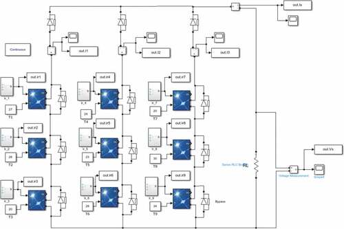
The simulation was carried out with PV modules employing the following electrical parameters for standard test conditions (STC):

• Peak Power ($P_{max}$): 100 W

• Voltage at Max. power ($V_{MP}$): 18.7 V

• Current at Max. power ($I_{MP}$): 5.35 A

• Open Circuit Voltage ($V_{OC}$): 22.3 V

• Short-Circuit Current ($I_{CC}$): 5.69 A

• Cell number: 60

• Standard Test Conditions (STC): G = 1000 W/m^2; T = 25 °C

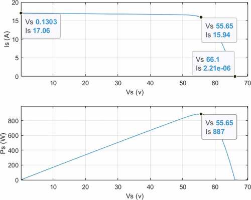
Figure 3 depicts the simulated system’s I–V and P-V curves for STC. It is evident that, under these conditions, the PV matrix had a maximum power of approximately 900 W.

Figure 3. PV matrix I–V (top) and P-V (bottom) plots for STC

Source: Authors’ own

3.2. Solution design

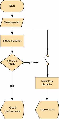
Figure 4 displays the solution for automatic fault detection in the PV matrix. The system was made up of two stages: first, a binary classifier to detect if there was a fault; second, a multiclass classifier to detect the type of fault, should there be one.

Figure 4. Solution’s flow diagram

Source: Authors’ own

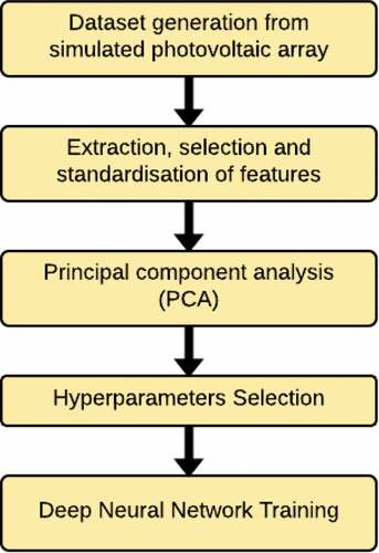
The solution was designed from the training of two artificial deep neural networks (DNN) for both classifiers. The training process was the same for both DNN and is presented in Figure 5.

Figure 5. DNN training procedure

Source: Authors’ own

The steps taken for each classifier are described below.

3.2.1. Dataset generation

The dataset was generated from different simulations where environmental conditions (irradiance and temperature), and charge resistance $R_L$ were randomly varied. Each simulation represented a day of operation where irradiance has a trapezoidal behavior, as shown in Figure 6. $G_{i,max}$ is different in each panel, and it was generated by a uniform probability distribution with a [600, 1400] $W/m^2$ range. Temperatures for each panel and each simulation were constant and changed between simulations with a uniform probability distribution and a [15,45] °C range. Lastly, the $R_L$ value was also kept constant during the simulation and then changed in-between, with a uniform probability distribution and a [1,100] Ω range.

Figure 6. Applied irradiance profile

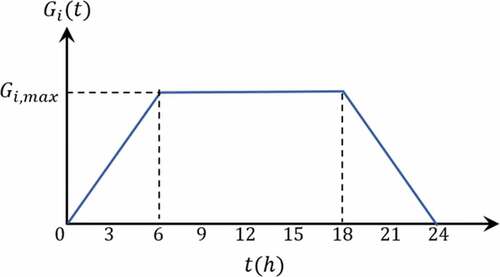
Each simulation represented irradiance behavior in a day. Samples were taken every 10 minutes, so a single simulation gave 144 samples for each of the 23 measured variables.

Since each simulation had a different probability distribution, it was essential to evaluate the system’s behavior with new simulations, that is, when new distributions appeared. Thus, two datasets were created, the first one to be used as training data while using both for validation and testing. In this work the system was tested with unknown probability distributions (second dataset).

For the correct functioning scenario (no faults), 300 simulations were carried out for the first dataset, and 30 for the second. For each of the nine faults, 100 simulations were carried out for the first dataset and 10 for the second.

Therefore, a dataset was created for the binary classifier with all no-fault functioning samples labeled ‘0ʹ, and all fault samples labeled ‘1ʹ. Here 30% of all fault samples was taken. Table 1 and 2 summarizes the dataset taken to train and evaluate the binary classifier in both sets.

Table 1. Methodologies for fault diagnosis in solar panels useful for this research

Proposed methodology by	Results
Chine et al., 2016	It can detect and classify eight different faults
Mekki et al., 2016	It can determine faults due to shades in the panel
De Benedetti et al., 2018	It can predict the power output from measured irradiance and temperature values
Rao et al., 2019	It can detect eight different faults
Pahwa et al., 2020	It can classify different failures

Table 2. Dataset for binary classifier

	Label	Sample number set 1	Sample number set 2
No fault	“0”	43.200	4.320
Fault	“1”	38.880	3.888
	Sample total	82.080	8.208

All the samples obtained from each fault were taken for the multiclass classifier. Table 3 presents the different detected faults, and the summary of the dataset used to train the multiclass classifier.

Table 3. Data set for multiclass classifier

Fault type	Label	Sample number set 1	Sample number set 2
Bypass diode short-circuit fault Column 3	“0”	14.400	1.440
Bypass diode short-circuit fault Column 2	“1”	14.400	1.440
Bypass diode short-circuit fault Column 1	“2”	14.400	1.440
Blocking diode short-circuit fault Column 3	“3”	14.400	1.440
Blocking diode short-circuit fault Column 2	“4”	14.400	1.440
Blocking diode short-circuit fault Column 1	“5”	14.400	1.440
Blocking diode open-circuit fault Column 3	“6”	14.400	1.440
Blocking diode open-circuit fault Column 2	“7”	14.400	1.440
Blocking diode open-circuit fault Column 1	“8”	14.400	1.440
	Sample total	129.600	12.960

3.2.2. Extraction, selection, and normalization of characteristics

Since the measured variables have a sequential nature (Figure 7), the extraction of characteristics was based on taking a certain number of samples preceding the measured sample, that is, characteristics are obtained for each variable from preceding samples, which help enhance the system’s accuracy. Consequently, the number of input characteristics for the two neural networks (binary and multiclass classifiers) depends on the number of preceding samples taken.

Figure 7. Extraction, selection and normalization flow

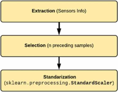
The only variables for which preceding samples were not considered are temperatures (T1, T2, T3, …, T9), as they were kept constant in each simulation. Thus, the number of input characteristics was given by equation 1(1) $n=14\mathit{\ast }{m}_{ant}+9$(1) :

(1) $n=14\mathit{\ast }{m}_{ant}+9$(1)

Where $n$ is the number of characteristics, and $m_{ant}$ is the number of preceding samples. The number 14 is due to having 9 irradiance variables (G1, G2, G3, …, G9), 4 current measurements (I1, I2, I3, Is) and the Vs voltage. The number 9 are the temperatures (T1, T2, T3, …, T9).

Because characteristics were found in very different ranges, the dataset obtained after the extraction and characteristic selection was normalized using the “preprocessing” package contained in Python’s “Scienty Kit Learn” (sklearn) framework.

3.2.3. Principal component analysis (PCA)

During system design, the two neural networks were shown to behave better as the number of preceding samples rose in the extraction of characteristics, though this also entailed an increase of computational load, and the times for both DNN training and prediction. As a result, the system’s complexity was reduced employing PCA, thus decreasing the number of characteristics without sacrificing the system’s accuracy. For this the “decomposition” package was used, also contained in Python’s “Scienty Kit Learn” (sklearn) framework.

3.2.4. Hyperparameter selection

Hyperparameter selection is summarized in Tables 4 and 5. These were adjusted based on the different training performed and on the system evaluation of accuracy with training, validation, and testing data. This selection was divided into two phases: the first consists in training and validation of models from datasets 1 and 2, respectively; in the second the model is tested with dataset 2.

Table 4. Hyperparameters selected for classifiers

Hyperparameter	Binary classifier	Multiclass classifier
Learning rate	0.001	0.0005
Number of Hidden layers	4	3
Hidden Layer Size	256	300
Batch size	1024	1024
$m_{ant}$	192	128
$n_{PCA}$	1536	1280

Table 5. Activation functions applied to classifiers

Layer ($l$)	Activation function $G_l\left(z\right)$
	Binary classifier	Multiclass classifier
1	$relu\left(z\right)$	$relu\left(z\right)$
2	$tanh\left(z\right)$	$relu\left(z\right)$
3	$relu\left(z\right)$	$relu\left(z\right)$
4	$tanh\left(z\right)$	$softmax\left(z\right)$
5	$sigmoid\left(z\right)$	–

Hyperparameters adjusted in the first phase were: Learning rate, number of hidden layers, batch size, and the activation function for each layer. While at the second phase the number of preceding samples ($m_{ant}$) and the number of characteristics after PCA ($n_{PCA}$) were adjusted.

3.2.5. Deep neural network training

The general architecture of DNN used in each classifier is shown in Figure 8,

Figure 8. Deep neural network architecture

Thus, the estimated output $\hat{Y}$ is the result of forward propagation and is given by:

(2) $\begin{array}{rl}& a_l=G_l\left(W_l{a}_{l-1}+b_l\hspace{0.17em}\right)forl=1,2,3,\dots ,L\\ & \stackrel{\mathit{ˆ}}{Y}=\left\{\begin{array}{cc}round\left(a_L\right)& \mathbf{f}\mathbf{o}\mathbf{r}\mathbf{b}\mathbf{i}\mathbf{n}\mathbf{a}\mathbf{r}\mathbf{y}\mathbf{c}\mathbf{l}\mathbf{a}\mathbf{s}\mathbf{s}\mathbf{i}\mathbf{f}\mathbf{i}\mathbf{e}\mathbf{r}\\ argmax\left(a_L\right)& \mathbf{f}\mathbf{o}\mathbf{r}\mathbf{m}\mathbf{u}\mathbf{l}\mathbf{t}\mathbf{i}\mathbf{c}\mathbf{l}\mathbf{a}\mathbf{s}\mathbf{s}\mathbf{c}\mathbf{l}\mathbf{a}\mathbf{s}\mathbf{s}\mathbf{i}\mathbf{f}\mathbf{i}\mathbf{e}\mathbf{r}\end{array}\right.\end{array}$(2)

Where $a_0=X$, $G_l\left(z\right)$ are activation functions for layer $l$, and $W_l$ and $b_l$ are the parameters (weight and bias, respectively) to be found through the training process of each layer $l$.

The optimal values of matrixes $W_l$ and of $b_l$ were found in a way such that the cost function $J$ was minimized (cross-entropy, equation 3)(3) $J=-\frac{1}{m}\sum _{i=0}^{m-1}{Y}^{\left(i\right)}log\left({\hat{Y}}^{\left(i\right)}\right)+\left(1-Y^{\left(i\right)}\right)log\left(1-{\hat{Y}}^{\left(i\right)}\right)$(3) :

(3) $J=-\frac{1}{m}\sum _{i=0}^{m-1}{Y}^{\left(i\right)}log\left({\hat{Y}}^{\left(i\right)}\right)+\left(1-Y^{\left(i\right)}\right)log\left(1-{\hat{Y}}^{\left(i\right)}\right)$(3)

Where, $Y^{\left(i\right)}$ are the labels and ${\hat{Y}}^{\left(i\right)\hspace{0.17em}}$are the predict values for the sample $i$.

The training was performed through batches, where m is the sample number per batch. The back-propagation and Adam optimization algorithms were applied with the assistance of Google Inc.’s Tensor Flow 2 framework.

4. Results

The results obtained were based on the system’s evaluation from the testing dataset. As mentioned before, the testing dataset came from a fresh set of simulations that was not used neither in training nor in validation.

System behavior drastically depended on hyperparameters: preceding samples and number of characteristics after PCA are interrelated in Table 4.

The results obtained in the training and testing process of the two models are detailed separately below, using accuracy as the main criterion. The results of the binary classifier are presented first and then those of the multiclass classifier.

4.1. Binary classifier

4.1.1. Data transformation

This classifier’s behavior heavily depended on the number of characteristics used, so different training was performed varying the number of characteristics according to the following hyperparameters: number of preceding samples ($m_{ant}$) and number of characteristics after PCA ($n_{PCA}$).

Table 6 presents the number of characteristics $n_{ant}$ before PCA based on the selected preceding samples $m_{ant}$ acquired from equation 1(1) $n=14\mathit{\ast }{m}_{ant}+9$(1) .

Table 6. Number of characteristics before PCA for binary classifier

$m_{ant}$	16	32	64	128	192
$n_{ant}$	233	457	905	1801	2697

Table 7 summarizes the system’s accuracy dependent on $m_{ANT}$ and $n_{ant}$. Logically, as these two hyperparameters grow, the computational cost grows even more so; the PCA process becomes too slow or unfeasible because of RAM resources.

Table 7. Accuracy of binary classifier for different $m_{ant}$ and $n_{PCA}$

$n_{PCA}$	$m_{ant}$
	16	32	64	128	192
128	71.22%	73.54%	78.05%	88.47%	90.25%
256	na	75.36%	79.46%	90.12%	91.45%
512	na	na	80.32%	91.07%	92.12%
768	na	na	80.54%	91.44%	92.85%
1024	na	na	na	91.67%	93.45%
1280	na	na	na	92.01%	94.42%
1536	na	na	na	92.11%	95.55%
1792	na	na	na	92.16%	95.56%

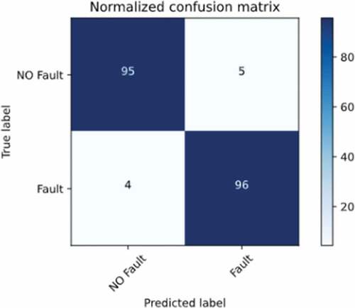
Thus, the selected values for m_ant and n_ant were 192 and 1536, respectively, with 95.55% accuracy for the testing dataset. The other hyperparameters are shown in Table 3, in the Hyperparameter selection section.

4.1.2. Training and validation

Figure 9 shows a normalized confusion matrix for the binary classifier with the testing dataset and the hyperparameters listed in Table 4.

Figure 9. Normalized confusion matrix for binary classifier

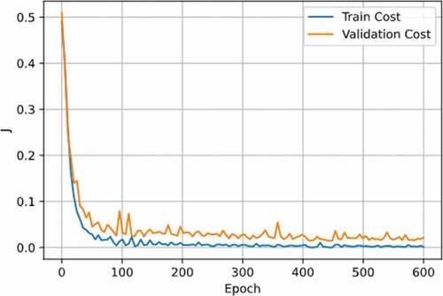
Lastly, Figure 10 shows the cost function during training. It can be seen that the model is not over-adjusted with validation data.

Figure 10. Training and validation cost in binary classifier

4.2. Multiclass classifier

4.2.1. Data transformation

Much like with the binary classifier, the multiclass classifier behavior greatly depended on the number of characteristics used. Consequently, both the process and selection of hyperparameters were carried out in the same way as for the binary classifier.

The number of characteristics n_ant before PCA based on the selected preceding samples m_ant is the same that the binary classifier (Table 6) acquired from equation 1(1) $n=14\mathit{\ast }{m}_{ant}+9$(1) .

The system’s accuracy dependency on m_ant and n_ant appears in Table 8.

Table 8. Accuracy of multiclass classifier for different m_ANT and n_PCA

nPCA	mant
	16	32	64	128	192
128	74.32%	78.26%	83.87%	91.54%	92.54%
256	n/a	80.24%	86.54%	92.64%	93.15%
512	n/a	n/a	87.46%	94.04%	94.25%
768	n/a	n/a	89.25%	96.89%	97.15%
1024	n/a	n/a	n/a	97.25%	97.30%
1280	n/a	n/a	n/a	97.28%	97.32%
1536	n/a	n/a	n/a	97.29%	97.32%
1792	n/a	n/a	n/a	97.31%	97.33%

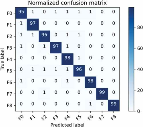
Thus, the selected $m_{ant}$ and $n_{ant}$ values were 128 y 1280, respectively, with 97.28% accuracy for the testing dataset. The other hyperparameters are shown in Table 3, in the Hyperparameter selection section.

4.2.2. Training and validation

Figure 11 shows a normalized confusion matrix for the multiclass classifier with the testing dataset and the hyperparameters listed in Table 4.

Figure 11. Normalized confusion matrix for multiclass classifier

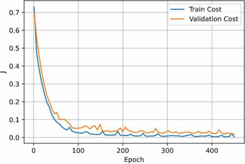
Figure 12. shows the cost function during training. It can be seen that the model is not overadjusted with validation data.

Figure 12. Training and validation cost in multiclass classifier

4.2.3. Summary of the two classifiers

Table 9 summarises the measurements for training and validation of both classifiers with the selected hyperparameters.

Table 9. Classifier evaluation measurements for training and validation

Measurement	Classifier
	Binary	Multiclass
Epoch number	600	450
Train cost	0.0013	0.0034
Validation cost	0.0210	0.0265
Train Accuracy	99.97%	99.89%
Validation Accuracy	98.75%	98.63%

4.2.4. Test

Finally, Figure 13 to 16 display pictures of the application working and linked with Matlab’s Simulink.

Figure 13. No-fault simulation where no faults are predicted

Figure 14 shows a prediction of short-circuit fault at column 2’s blocking diode.

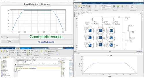
Figure 14. Fault simulation where short-circuit faults are predicted at column 2’s blocking diode

Figure 15 depicts the prediction of an open circuit fault at column 3’s blocking diode.

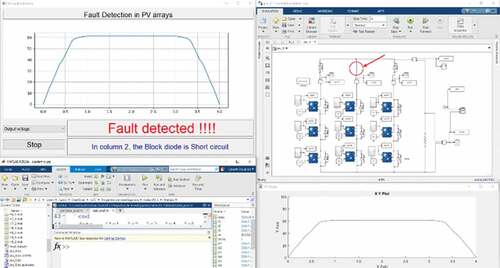
Figure 15. Fault simulation where open circuit faults are predicted at column 3’s blocking diode

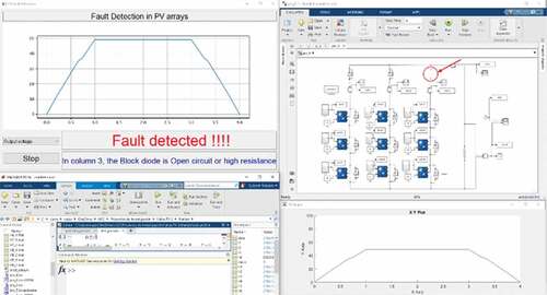
Figure 16. Fault simulation where short-circuit faults are predicted at column 1’s bypass diode

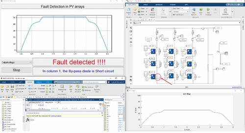
Lastly, Figure 16 exhibits the system with a fault at one of column 1’s bypass diodes.

Figure 13 shows a system with no faults where the model makes a correct “no faults” prediction.

This link: https://youtu.be/G6RNaqiK7-c presents a video demonstration of the performance of the research.

5. Conclusions

In general, the proposed methodology was shown to be reliably able to detect faults, it shows that the problem for automatic fault detection can be divided into two parts: first, it is detected if there are faults, and then the fault type is detected. Figure 10 and 12, as well as Table 8, showed that none of the classifiers are overfitting. The variance between training and validation costs is very low, which implies standardisation is not necessary. Also, the evaluation of the models obtained shows that the transformation of the data, such as the inclusion of the previous samples, enabled a considerable increase in the accuracy. Tables 6 and 7 show the improvement of the system as the number of previous samples increases for binary and multiclass classifiers. Additionally, the use of PCA allows the computational cost to be reduced. Finally, the binary and multiclass classifiers have accuracies of 95.55% and 97.28%, respectively, with a total accuracy of 92.95%.

This methodology is intended to be implemented in Colombia, in zones with difficult access and without interconnection to the electricity grid and seeks to reduce corrective maintenance.

Acknowledgements

This study is part of the Project “Enhancing Aquatic Renewable Energy (ARE): Technology design and adaptation program for Colombia” (IAPP18-19\90) funded by the Newton Fund/Royal Academy of Engineering under the Industry Academy Partnership Programme. In addition, the authors would like to thank the partners of the ENCORE (Energizing Coastal Regions with Offshore Renewable Energy) project for fruitful discussions and sharing some ideas about offshore renewable energy. ENCORE receives funding from theInterreg 2 Seas programme 2014-2020, co-funded by the European Regional Development Fund under subsidy contract No 2S08-004. The provinces of South and North Holland and Zeeland are also offering financial support.

The support of the Institute for Planning and Promotion of Energy Solutions for Non-Interconnected Zones (IPSE) of the Colombian Ministry of Mines and Energy is also acknowledged. 

Disclosure statement

No potential conflict of interest was reported by the author(s).

Additional information

Funding

This study is part of the Project “Enhancing Aquatic Renewable Energy (ARE): Technology design and adaptation program for Colombia” (IAPP18-19\90) funded by the Newton Fund/Royal Academy of Engineering under the Industry Academy Partnership Programme (IAPP).

Notes on contributors

Ramón Fernando Colmenares-Quintero

Ramón Fernando Colmenares-Quintero is currently national head of research in engineering and Professor Dr. at UCC with research focus on energy generation, simulation and modelling in the energy sector and vulnerable communities.Eyberth R. Rojas-Martinez is an electronic engineer graduated from Santo Tomás University and a Master in Electronic Engineering from the National University of Colombia. With experience in mathematical models based on machine learning techniques.Fernando Macho is Managing Partner of SEC which is a consulting firm in Spain, whose main aim is to advise on international matters and foreign trade.Kim E. Stansfield got a PhD in Composites from Kingston University. He was sustainable energy systems transformation planner at the UK ETI. Joined Warwick WMG in 2016. Prof. Dr. Juan Carlos Colmenares-Quintero is the leader of the research group CatSEE from the IPC/PAS in Poland. His interests range from materials science/nanotechnology to photocatalysis and water/air purification.

References

- Ahmed, B. M., & Farman Alhialy, N. F. (2019). Optimum efficiency of PV panel using genetic algorithms to Touch Proximate Zero Energy House (NZEH). Civil Engineering Journal, 5(8), 1832–21. https://doi.org/10.28991/cej-2019-03091375
- Bonsignore, L., Davarifar, M., Rabhi, A., Tina, G. M., & Elhajjaji, A. (2014). Neuro-Fuzzy fault detection method for photovoltaic systems. Energy Procedia, 62, 431–441. https://doi.org/10.1016/j.egypro.2014.12.405
- Chen, Z., Chen, Y., Wu, L., Cheng, S., & Lin, P. (2019). Deep residual network based fault detection and diagnosis of photovoltaic arrays using current-voltage curves and ambient conditions. Energy Conversion and Management, 198, 111793. https://doi.org/10.1016/j.enconman.2019.111793
- Chine, W., Mellit, A., Lughi, V., Malek, A., Sulligoi, G., & Massi Pavan, A. (2016). A novel fault diagnosis technique for photovoltaic systems based on artificial neural networks. Renewable Energy, 90, 501–512. https://doi.org/10.1016/j.renene.2016.01.036
- Chine, W., Mellit, A., Pavan, A. M., & Kalogirou, S. A. (2014). Fault detection method for grid-connected photovoltaic plants. Renewable Energy, 66, 99–110. https://doi.org/10.1016/j.renene.2013.11.073
- De Benedetti, M., Leonardi, F., Messina, F., Santoro, C., & Vasilakos, A. (2018). Anomaly detection and predictive maintenance for photovoltaic systems. Neurocomputing, 310, 59–68. https://doi.org/10.1016/j.neucom.2018.05.017
- Dhimish, M., Holmes, V., Mehrdadi, B., & Dales, M. (2018). Comparing Mamdani Sugeno fuzzy logic and RBF ANN network for PV fault detection. Renewable Energy, 117, 257–274. https://doi.org/10.1016/j.renene.2017.10.066
- Firth, S. K., Lomas, K. J., & Rees, S. J. (2010). A simple model of PV system performance and its use in fault detection. Solar Energy, 84(4), 624–635. https://doi.org/10.1016/j.solener.2009.08.004
- Harrou, F., Sun, Y., Taghezouit, B., Saidi, A., & Hamlati, M.-E. (2018). Reliable fault detection and diagnosis of photovoltaic systems based on statistical monitoring approaches. Renewable Energy, 116, 22–37. https://doi.org/10.1016/j.renene.2017.09.048
- Hosenuzzaman, M., Rahim, N. A., Selvaraj, J., Hasanuzzaman, M., Malek, A. B. M. A., & Nahar, A. (2015). Global prospects, progress, policies, and environmental impact of solar photovoltaic power generation. Renewable and Sustainable Energy Reviews, 41, 284–297. https://doi.org/10.1016/j.rser.2014.08.046
- Jiang, L. L., & Maskell, D. L. (2015). Automatic fault detection and diagnosis for photovoltaic systems using combined artificial neural network and analytical based methods. 2015 International Joint Conference on Neural Networks (IJCNN), 1–8, Killarney, Ireland. https://doi.org/10.1109/IJCNN.2015.7280498
- Kibaara, S. K., Murage, D. K., Musau, P., & Saulo, M. J. (2020). Comparative analysis of implementation of solar PV systems using the advanced SPECA modelling tool and HOMER software: Kenyan scenario. HighTech and Innovation Journal, 1(1), 8–20. https://doi.org/10.28991/HIJ-2020-01-01-02
- Lu, X., Lin, P., Cheng, S., Lin, Y., Chen, Z., Wu, L., & Zheng, Q. (2019). Fault diagnosis for photovoltaic array based on convolutional neural network and electrical time series graph. Energy Conversion and Management, 196, 950–965. https://doi.org/10.1016/j.enconman.2019.06.062
- Madeti, S. R., & Singh, S. N. (2018). Modeling of PV system based on experimental data for fault detection using kNN method. Solar Energy, 173, 139–151. https://doi.org/10.1016/j.solener.2018.07.038
- Mekki, H., Mellit, A., & Salhi, H. (2016). Artificial neural network-based modelling and fault detection of partial shaded photovoltaic modules. Simulation Modelling Practice and Theory, 67, 1–13. https://doi.org/10.1016/j.simpat.2016.05.005
- Pahwa, K., Sharma, M., Saggu, M. S., & Mandpura, A. K. (2020, February). Performance evaluation of machine learning techniques for fault detection and classification in PV array systems. In 2020 7th International Conference on Signal Processing and Integrated Networks (SPIN) (pp. 791–796). IEEE, Noida, India.
- Pierdicca, R., Malinverni, E. S., Piccinini, F., Paolanti, M., Felicetti, A., & Zingaretti, P. (2018). DEEP CONVOLUTIONAL NEURAL NETWORK FOR AUTOMATIC DETECTION OF DAMAGED PHOTOVOLTAIC CELLS. ISPRS - International Archives of the Photogrammetry, Remote Sensing and Spatial Information Sciences, XLII–2, XLII-2, 893–900. https://doi.org/10.5194/isprs-archives-XLII-2-893-2018
- Rao, S., Spanias, A., & Tepedelenlioglu, C. (2019). Solar array fault detection using neural networks. 2019 IEEE International Conference on Industrial Cyber Physical Systems (ICPS), 196–200, Taipei, Taiwan. https://doi.org/10.1109/ICPHYS.2019.8780208
- Solórzano, J., & Egido, M. A. (2014). Hot-spot mitigation in PV arrays with distributed MPPT (DMPPT). Solar Energy, 101, 131–137. https://doi.org/10.1016/j.solener.2013.12.020