On The Fractional Domain Analysis of HP TiO2 Memristor Based Circuits with Fractional Conformable Derivative

Abstract

For the first time, the physical memristor-based circuits i.e., HP TiO₂ memristor-based circuits, of both series and parallel structures, have been extensively analyzed in the fractional domain by means of the state of the art yet simple fractional conformable derivative-based differential equations. Different outcome from the hypotheticalmemory element-based previous researches have been obtained. The dimensional consistencies of the fractional derivatives have also been concerned. The often-cited Joglekar’s window function has been adopted for modelling the boundary effect of the memristor and adding more nonlinearity close to the bounds of the memristor’s state variable. The formulated fractional differential equations have been solved and the related electrical quantities have been determined. The computational simulations have been performed. The stability analyses of both circuits have also been presented where it has been mathematically verified that only these HP TiO₂ memristor-based circuits are stable always due to the boundary effect which does not exist in hypothetical elements assumed in those previous works. We also point out that that only those HP TiO₂ memristor-based circuits of order higher than 3 are capable to exhibit the complex dynamics as such memristor lacks the local activity.

Keywords:

• Fractional conformable derivative
• fractional differential equation
• fractional domain
• HP TiO₂ memristor
• nonlinear circuit

Subjects:

• Fractional calculus
• Electronic engineering
• Electrical engineering

PUBLIC INTEREST STATEMENT

Among various fractional derivatives, the fractional conformable derivative has been found to be one of the simplest yet maximally accurate for modelling the real-world physical systems e.g., real electrical circuits etc., which employs fractional characteristics thus cannot be accurately modelled be means of conventional calculus. Such fractional conformable derivative has been applied to the electrical circuits containing circuit elements with memories. However, only hypothetical elements with memories have been considered albeit there exists a physical one i.e., the HP TiO₂ memristor. Such HP TiO₂ memristor has been implemented at nanometer level by Hewlett Packard’s laboratory and is often cited in many previous works. Hence, the analysis of electrical circuits containing such physical element with memory has been performed in this work based on the mentioned fractional conformable derivative.

1. Introduction

The fractional calculus which is the extension of the conventional integer calculus has been extensively utilized in various research areas e.g., signal processing (R. Panda & Dash, 2006), (Yang & Zhou, 2008), biomedical engineering (Sommacal et al., 2008), (Magin & Ovadia, 2008), electronics (Pu et al., 2006), (Krishna et al., 2008), (Carreño et al., 2019) robotics (Rosario et al., 2006), (Lima et al., 2007) and control theory (Deng et al., 2007), (Cervera & Baños, 2008), (Bohannan, 2008) etc. The fractional differential equation (FDE) has been used in the fractional domain analysis of both linear and nonlinear electrical circuits (Ayoub et al., 2006), (Cafagna & Grassi, 2012), (Gómez et al., 2013), (Guía et al., 2013), (Francisco et al., 2014), (Shah et al., 2014), (Atangana & Alkahtani, 2015), (Gómez‐Aguilar et al., 2017), (Martínez et al., 2018), (Ruan et al., 2018), (He et al., 2018), (Y. Yu et al., 2019). Such fractional domain analysis has been found to be necessary because the electrical circuit components in practice have irreversible dissipative effects e.g., ohmic friction, thermal memory, and electromagnetic field induced nonlinearities etc., which cannot be precisely analyzed in the conventional integer domain.

Recently, many novel definitions of the fractional derivative have been proposed e.g., the fractional conformable derivative (Khalil et al., 2014), Caputo–Fabrizio (Caputo & Fabrizio, 2015), Atangana–Baleanu (Atangana & Baleanu, 2016) and generalized fractional derivative (Jarad et al., 2017) etc. The FDEs formulated by these new derivatives have been used in the fractional domain analysis of electrical circuits (Atangana & Alkahtani, 2015), (Gómez‐Aguilar et al., 2017), (Martínez et al., 2018), (Ruan et al., 2018), (He et al., 2018), (Sene, 2020). Compared with other fractional operators, the fractional conformable derivative provides more simplicity due to its consistency with the conventional derivative which does not exist in the other fractional derivative’s definitions (Martínez et al., 2018), and maximum accuracy in real world fractional domain circuit modelling (Carreño et al., 2019). The FDEs formulated by such fractional conformable derivative have been applied to linear electrical circuit (Martínez et al., 2018). For nonlinear circuits on the other hand, those circuits with hypothetical memory circuit elements have been studied (Ruan et al., 2018), (He et al., 2018). In fact, there exists a physical circuit element with memory i.e., the HP TiO₂ memristor, which has been implemented at nanometer level by Hewlett Packard’s laboratory (Strukov et al., 2008). This HP TiO₂ memristor has been dedicated to by many previous works in the fractional domain (Fouda & Radwan, 2013), (Fouda & Radwan, 2015), (Y.J. Yu et al., 2015), (Shi & Hu, 2017), (Banchuin, 2018), (Banchuin & Konofaos, 2021), (Banchuin & Meng, 2021). To the best of our knowledge, the analysis of nonlinear circuit with physical memory circuit element such as the HP TiO₂ memristor based on the fractional conformable derivative has never been performed despite the interesting applications of HP TiO₂ memristor e.g., oscillator (Talukdar et al., 2011), and chaotic circuit (Wang, Sun, et. al., 2018a), (Wang, Sun, et al., 2018bMay) etc.

Hence, the fractional domain analysis of the HP TiO₂ memristor-based circuits by using the fractional conformable derivative-based FDEs have been proposed for the first time in this work. The fractional conformable derivative is of interest because of its abovementioned virtues. Both nonlinear circuits are respectively the series and parallel combination of HP TiO₂ memristor, inductor and capacitor. They have been chosen as they are the HP TiO₂ memristor-based counterparts of simple series and parallel circuits composed of resistor, inductor and capacitor which are the supersets of most circuits considered in the aforesaid previous works and serve as the common fundamental building blocks in electrical engineering. The dimensional consistencies of the fractional derivatives have also been considered similar to (Martínez et al., 2018), (Sene, 2019), (Sene, 2020) and (Banchuin, 2021) but unlike (Ruan et al., 2018) and (He et al., 2018). In addition, we directly apply the relationship between the fractional conformable derivative and the conventional one as proposed by Khalil et al. (Khalil et al., 2014) due to its simplicity. This is also unlike Ruan et al. and He et al. Compared with those schemes dedicated to the fractional conformable derivative-based FDE with partial derivative terms with such as Adomian decomposition method in conformable sense (Yavuz & Yaşkıran, 2017), modified homopoty perturbation method in conformable sense (Yavuz & Yaşkıran, 2018), conformable fractional modified homotopy perturbation method (Yavuz, 2018) and conformable separate homotopy method (Yavuz, 2019), our chosen methodology has been found to be much more convenient beside its adequacy for our work as the associated equations contain no such cumbersome partial derivative. The often-cited Joglekar’s window function (Joglekar & Wolf, 2009) has been adopted for modelling the boundary effect of the HP TiO₂ memristor, which does not exist in those hypothetical memory circuit elements adopted by Ruan et al. and He et al., and adding more nonlinearity close to the bounds of the memristor’s state variable. The formulated FDEs have been solved and the related electrical quantities have been determined based on the obtained solutions. By using the numerical simulations with MATHEMATICA, the dynamical behaviors of these circuits in the fractional domain under various types of excitations including zero, DC and AC signals have been studied in detail. In particular, the effect of extending each circuit element to fractional domain by allowing the associated order of the FDE to become fractional have been studied. The analytical stability analyses of the circuits have also been presented where it has been verified that these circuits are stable always due to the boundary effect of the HP TiO₂ memristor, which does not exist in hypothetical elements assumed by Ruan et al. and He et al. We also point out that only those HP TiO₂ memristor-based circuits of order higher than 3 are capable to exhibit the complex dynamics as such memristor lacks the local activity. If a 3^rd order circuit is desired, a locally active memristor must be adopted.

2. Overview of fractional conformable derivative

Definition 1 (Khalil et al., 2014): Let g(u) be arbitrary function and $u\in {\mathrm{\Re }}^{+}$. The fractional conformable derivative of g(u) (${\mathrm{D}}^{\lambda }[g(u)]),$ can be mathematically defined as

(1) ${\mathrm{D}}^{\lambda }[g(u)]=\underset{\epsilon \to 0}{lim}[\frac{g(u+\epsilon u^{1-\lambda })-g(u)}{\epsilon }]$(1)

where λ denotes the order of such derivative and 0 < λ < 1.

Corollary 1: If we let λ = 1, ${\mathrm{D}}^{\lambda }[g(u)]=\frac{\mathrm{d}g(u)}{\mathrm{d}u}$where $\frac{\mathrm{d}g(u)}{\mathrm{d}u}$stands for the conventional derivative of g(u).

According to (Khalil et al., 2014), the fractional conformable derivative shares many common properties with the conventional derivative. Therefore, the mathematical analysis involving the fractional conformable derivative become relatively acquainted as because the knowledge on classical calculus can be applied. Moreover, the following relationship between the fractional conformable derivative and the conventional one has been found to be very useful.

Theorem 1(Khalil et al., 2014): If $\frac{\mathrm{d}g(u)}{\mathrm{d}u}$ exists, we have

(2) ${\mathrm{D}}^{\lambda }[g(u)]=u^{1-\lambda }\frac{\mathrm{d}g(u)}{\mathrm{d}u}$(2)

See (Khalil et al., 2014) for the proof of theorem 1.

3. Foundation on HP TiO₂ memristor

Regardless to the implementation, the memristor is a nonlinear electrical circuit element that relates the instantaneous flux (ϕ(t)) and charge (q(t)) through the following relationship

where M(t) denotes the memristance.

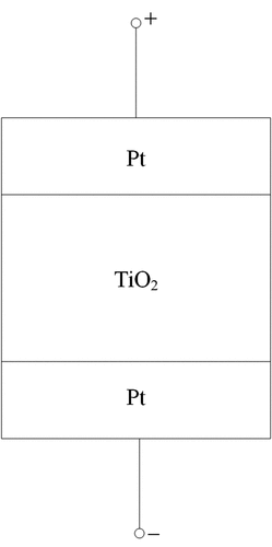
For the HP TiO₂ memristor, which is composed of a TiO₂ layer between two platinum electrodes as can be seen from Figure 1, its M(t) can be given in terms of the minimum and maximum values of M(t) denoted by M_on and M_off and the state variable (x(t)) as (Strukov et al., 2008)

(4) $M(t)=M_{on}x(t)+(1-x(t))M_{off}$(4)

Figure 1. The physical schematic diagram of HP TiO₂ memristor

where x(t) which is dimensionless, can be given in term of the memristor’s current (i(t)) by

(5) $\frac{dx(t)}{dt}=ki(t)$(5)

Noted that k = μM_on/D² where μ and D, respectively, stand for the ion mobility and semiconductor film of thickness. Therefore, the dimension of k is (A∙s)⁻¹.

By the boundary effect of this device, M_on ≤ M(t) ≤ M_off always as 0 ≤ x(t) ≤ 1. At the saturation state, M(t) can be either M_on when x(t) = 0 or M_off when x(t) = 1. For mathematically incorporating such boundary effect in a compact manner and adding more nonlinearity close to the bounds of x(t), the window function (f(x(t)) which is a function of x(t), must be introduced as stated above. As a result, equation (5)(5) $\frac{dx(t)}{dt}=ki(t)$(5) becomes

(6) $\frac{dx(t)}{dt}=ki(t)f(x(t))$(6)

In this work, the Joglekar’s window function has been assumed for modelling such boundary effect as it is often cited previous works on the modeling of HP TiO₂ memristor (Biolek, Biolek, et al., 2009a, August), (Biolek, Biolek et al., 2009b), (Biolek et al., 2014). As a result, we have

(7) $\frac{dx(t)}{dt}=ki(t)(1-(2x(t)-1{)}^{2p})$(7)

where$p\in {\mathbf{Z}}^{+}$.

4. HP TiO₂ memristor-based circuits in the fractional domain

Consider a series combination of HP TiO₂ memristor, inductor and capacitor depicted in Figure 2. After performing the rigorous circuit analysis with the aid of equations (4)(4) $M(t)=M_{on}x(t)+(1-x(t))M_{off}$(4) and (7(7) $\frac{dx(t)}{dt}=ki(t)(1-(2x(t)-1{)}^{2p})$(7) ), the following system of ODEs can be obtained

$\frac{\mathrm{d}x(t)}{\mathrm{d}t}=ki(t)(1-(2x(t)-1{)}^{2p})$

$\frac{\mathrm{d}i(t)}{\mathrm{d}t}=-(M_{on}x(t)+(1-x(t))M_{off})L_i^{-1}(t)-C^{-1}{L}_q^{-1}(t)+L_v^{-1}(t)$

(8) $\frac{\mathrm{d}q(t)}{\mathrm{d}t}=i(t)$(8)

Figure 2. The series HP TiO₂ memristor based circuit

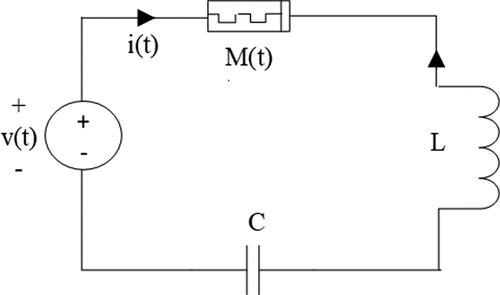
where i(t), q(t) and v(t) denote the current response of the circuit which flowing through all circuit elements, stored capacitive charge and exciting voltage, respectively.

For the extension to fractional domain, all conventional derivatives within equation (8)(8) $\frac{\mathrm{d}q(t)}{\mathrm{d}t}=i(t)$(8) must be replaced by the fractional ones where incommensurate orders have been assumed for more degree of freedom. Since the dimensional consistencies of the fractional derivatives, which are respected to t, have also been considered, the fractional time component parameter or the cosmic time (σ) (Gómez-Aguilar et al., 2012) must be included in the fractional derivative terms of the resulting system of FDEs. As a result, we have

${\sigma }_{\hspace{0.17em}}^{\alpha -1}{\mathrm{D}}^{\alpha }[x(t)]=ki(t)(1-(2x(t)-1{)}^{2p})$

(9) ${\sigma }_{\hspace{0.17em}}^{\beta -1}{\mathrm{D}}^{\beta }[q(t)]=i(t)$(9)

${\sigma }_{\hspace{0.17em}}^{\gamma -1}{\mathrm{D}}^{\gamma }[i(t)]=-(M_{on}x(t)+(1-x(t))M_{off})L_{\hspace{0.17em}}^{-1}i(t)-C^{-1}{L}_{\hspace{0.17em}}^{-1}q(t)+L_{\hspace{0.17em}}^{-1}v(t)$

where 0 < α < 1, 0 < β < 1 and 0 < γ < 1.

After some rearrangement, the following system of FDE can be obtained

${\mathrm{D}}^{\alpha }[x(t)]=k_{\alpha }i(t)(1-(2x(t)-1{)}^{2p})$

(10) ${\mathrm{D}}^{\beta }[y(t)]=i(t)$(10)

${\mathrm{D}}^{\gamma }[i(t)]=-(M_{on}x(t)+(1-x(t))M_{off})L_{\gamma }^{-1}i(t)-C_{\beta }^{-1}{L}_{\gamma }^{-1}y(t)+L_{\gamma }^{-1}v(t)$

where $y(t)=q(t){\sigma }_{\hspace{0.17em}}^{\beta -1}$, k_α = kσ^1-α, C_β = Cσ^β−1 and L_γ = Lσ^γ−1. Noted also that the dimensions of y(t), k_α, C_β and L_γ are C∙s^β−1, A⁻¹∙s^−α, F∙s^β−1 and H∙s^γ−1, respectively as σ has the dimension of s. In electrical engineering terms, C_β and L_γ are, respectively, referred to as the pseudo capacitance (Freeborn et al., 2013) and the inductivity (Schäfer & Krüger, 2006). Since σ must be assigned with a unique physical meaning depending on the circuit under consideration, we let our σ for both series and parallel circuits be physically the fraction of reciprocal of their associated undamped natural frequencies as the dimensions of such reciprocals are time. The closed form expressions of σ of both circuits will be derived later.

Since the fractional conformable derivative has been adopted, equation (10)(10) ${\mathrm{D}}^{\beta }[y(t)]=i(t)$(10) can be solved in a simplified manner with the aid of theorem 1 as the causality has been assumed. As a result, we have

$\frac{\mathrm{d}x(t)}{\mathrm{d}t}=k_{\alpha }{t}^{\alpha -1}i(t)(1-(2x(t)-1{)}^{2p})$

(11) $\frac{\mathrm{d}y(t)}{\mathrm{d}t}=t^{\beta -1}i(t)$(11)

$\frac{\mathrm{d}\mathrm{i}(\mathrm{t})}{\mathrm{d}t}=-(M_{on}x(t)+(1-x(t))M_{off})L_{\gamma }^{-1}{t}^{\gamma -1}i(t)-C_{\beta }^{-1}{L}_{\gamma }^{-1}{t}^{\gamma -1}y(t)+L_{\gamma }^{-1}{t}^{\gamma -1}v(t)$

which can be rearranged in a matrix-vector format as follows

(12) $\frac{d\mathbf{x}(t)}{dt}=\mathbf{A}(t,\mathbf{x}(t))\mathbf{x}(t)+\mathbf{b}(t)$(12)

where $\mathbf{x}(t)=[\begin{array}{ccc}x(t)& y(t)& i(t)\end{array}{]}^T$, $\mathbf{b}(t)=[\begin{array}{ccc}0& 0& L_{\gamma }^{-1}{t}^{\gamma -1}v(t)\end{array}{]}^T$

and$\mathbf{A}(t,\mathbf{x}(t))=\left[\begin{array}{ccc}0& 0& k_{\alpha }{t}^{\alpha -1}(1-{(2x(t)-1)}^{2p})\\ 0& 0& t^{\beta -1}\\ 0& -C_{\beta }^{-1}{L}_{\gamma }^{-1}{t}^{\gamma -1}& -(M_{on}x(t)+(1-x(t))M_{off})L_{\gamma }^{-1}{t}^{\gamma -1}\end{array}\right]$ .

After solving (12), we have

(13) $\mathbf{x}(t)=\mathbf{x}(0)+\underset{0}{\overset{t}{\int }}\mathbf{A}(\tau ,\mathbf{x}(\tau ))\mathbf{x}(\tau )d\tau +\underset{0}{\overset{t}{\int }}\mathbf{b}(\tau )d\tau$(13)

Since equation (12)(12) $\frac{d\mathbf{x}(t)}{dt}=\mathbf{A}(t,\mathbf{x}(t))\mathbf{x}(t)+\mathbf{b}(t)$(12) has been found to be the equivalent matrix-vector ODE of equation (10)(10) ${\mathrm{D}}^{\beta }[y(t)]=i(t)$(10) , the solution of equation (10)(10) ${\mathrm{D}}^{\beta }[y(t)]=i(t)$(10) can be obtained from that of equation (12)(12) $\frac{d\mathbf{x}(t)}{dt}=\mathbf{A}(t,\mathbf{x}(t))\mathbf{x}(t)+\mathbf{b}(t)$(12) i.e., equation (13)(13) $\mathbf{x}(t)=\mathbf{x}(0)+\underset{0}{\overset{t}{\int }}\mathbf{A}(\tau ,\mathbf{x}(\tau ))\mathbf{x}(\tau )d\tau +\underset{0}{\overset{t}{\int }}\mathbf{b}(\tau )d\tau$(13) . Therefore, x(t), y(t) and i(t) can be, respectively, given by x[1,1], x[2,1] and x[3,1]. If we let the circuit be, respectively, subjected to zero, DC and AC exciting signals i.e., v(t) = 0, v(t) = Vu(t) where u(t) stands for unit step function and v(t) = Vsin(ωt+ϴ), we, respectively, obtain $\underset{0}{\overset{t}{\int }}\mathbf{b}(\tau )d\tau =[\begin{array}{ccc}0& 0& 0\end{array}{]}^T$, $\underset{0}{\overset{t}{\int }}\mathbf{b}(\tau )d\tau =[\begin{array}{ccc}0& 0& {\gamma }^{-1}V{t}^{\gamma }\end{array}{]}^T$ and $\begin{array}{rl}& \underset{0}{\overset{t}{\int }}\mathbf{b}(\tau )d\tau =\left[\begin{array}{c}0\\ 0\\ L_{\gamma }^{-1}V{t}^{\gamma }[\frac{{\hspace{0.17em}}_1{\mathrm{F}}_2(\frac{\gamma }{2};\frac{1}{2},\frac{\gamma }{2}+2;-\frac{{(\omega t)}^2}{4})sin(\theta )}{\gamma }+\frac{\omega t{\hspace{0.17em}}_1{F}_2(\frac{\gamma +1}{2};\frac{3}{2},\frac{\gamma +3}{2};-\frac{{(\omega t)}^2}{4})cos(\theta )}{\gamma +1}]\end{array}\right]\end{array}$

where ₁F₂(;,;) denotes a generalized hypergeometric function with p = 1 and q = 2 (Dwork, 1990).

After determining x(t), y(t) and i(t), M(t) can be immediately obtained by using equation (4)(4) $M(t)=M_{on}x(t)+(1-x(t))M_{off}$(4) and x(t). As a result, the voltage dropped across the memristor (v_M(t)) can be found as

(14) $v_M(t)=M(t)i(t)$(14)

On the other hand, the voltage dropped across the capacitor ($v_{C_{\beta }}(t)$) can be found as

(15) $v_{C_{\beta }}(t)=C_{\beta }^{-1}y(t)$(15)

Therefore, the voltage dropped across the inductor ($v_{L_{\gamma }}(t)$) can be obtained by applying the Kirchhoff’s voltage law as follows

(16) $v_{L_{\gamma }}(t)=v(t)-M(t)i(t)-C_{\beta }^{-1}y(t)$(16)

Now, consider the parallel combination of memristor, inductor and capacitor depicted in Figure 3. For this parallel, HP TiO₂ memristor-based circuit, we have

$\frac{\mathrm{d}x(t)}{\mathrm{d}t}=\frac{kv(t)(1-{(2x(t)-1)}^{2p})}{M_{on}x(t)+(1-x(t))M_{off}}$

(17) $\frac{\mathrm{d}v(t)}{\mathrm{d}t}\hspace{0.17em}=-\frac{v(t)}{[M_{on}x(t)+(1-x(t))M_{off}]C}-\frac{\phi (t)}{LC}+\frac{i(t)}{C}$(17)

$\frac{\mathrm{d}\phi (t)}{\mathrm{d}t}=v(t)$

Figure 3. The parallel HP TiO₂ memristor based circuit

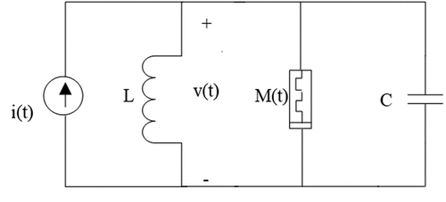
where i(t) and v(t) are now the current excitation and the voltage response of the circuit which dropped across all circuit elements, respectively. Note also that $\phi (t)$ stands for the inductive flux.

After the extension to fractional domain by keeping the dimensional consistencies of fractional derivative terms in mind, the obtained system of FDE can be given by equation (18)(18) ${\mathrm{D}}^{\beta }[v(t)]=-\frac{v(t)}{[M_{on}x(t)+(1-x(t))M_{off}]C_{\beta }}-\frac{z(t)}{L_{\gamma }{C}_{\beta }}+\frac{i(t)}{C_{\beta }}$(18) where $z(t)=\phi (t){\sigma }_{\hspace{0.17em}}^{\gamma -1}$ thus the dimension of z(t) is Wb∙s^γ−1.

${\mathrm{D}}^{\alpha }[x(t)]=\frac{k_{\alpha }v(t)(1-{(2x(t)-1)}^{2p})}{M_{on}x(t)+(1-x(t))M_{off}}$

(18) ${\mathrm{D}}^{\beta }[v(t)]=-\frac{v(t)}{[M_{on}x(t)+(1-x(t))M_{off}]C_{\beta }}-\frac{z(t)}{L_{\gamma }{C}_{\beta }}+\frac{i(t)}{C_{\beta }}$(18)

${\mathrm{D}}^{\gamma }[z(t)]=v(t)$

Since the fractional conformable derivative and causality has been assumed, equation (18)(18) ${\mathrm{D}}^{\beta }[v(t)]=-\frac{v(t)}{[M_{on}x(t)+(1-x(t))M_{off}]C_{\beta }}-\frac{z(t)}{L_{\gamma }{C}_{\beta }}+\frac{i(t)}{C_{\beta }}$(18) can be reformulated with the aid of theorem 1 as

$\frac{\mathrm{d}x(t)}{\mathrm{d}t}=\frac{k_{\alpha }{t}^{\alpha -1}v(t)(1-{(2x(t)-1)}^{2p})}{M_{on}x(t)+(1-x(t))M_{off}}$

(19) $\frac{\mathrm{d}v(t)}{\mathrm{d}t}=-\frac{t^{\beta -1}v(t)}{[M_{on}x(t)+(1-x(t))M_{off}]C_{\beta }}-\frac{t^{\beta -1}}{L_{\gamma }{C}_{\beta }}z(t)+\frac{t^{\beta -1}}{C_{\beta }}i(t)$(19)

$\frac{\mathrm{d}z(t)}{\mathrm{d}t}=t^{\gamma -1}v(t)$

which can be rearranged in a matrix-vector format as given by equation (12)(12) $\frac{d\mathbf{x}(t)}{dt}=\mathbf{A}(t,\mathbf{x}(t))\mathbf{x}(t)+\mathbf{b}(t)$(12) therefore its solution can also be given by equation (13)(13) $\mathbf{x}(t)=\mathbf{x}(0)+\underset{0}{\overset{t}{\int }}\mathbf{A}(\tau ,\mathbf{x}(\tau ))\mathbf{x}(\tau )d\tau +\underset{0}{\overset{t}{\int }}\mathbf{b}(\tau )d\tau$(13) . However, it must be kept in mind that $\mathbf{x}(t)=[\begin{array}{ccc}x(t)& v(t)& z(t)\end{array}{]}^T$, $\mathbf{b}(t)=[\begin{array}{ccc}0& C_{\beta }^{-1}{t}^{\beta -1}i(t)& 0\end{array}{]}^T$ and

$\mathbf{A}(t,\mathbf{x}(t))=\left[\begin{array}{ccc}0& \frac{k_{\alpha }{t}^{\alpha -1}(1-{(2x(t)-1)}^{2p})}{M_{on}x(t)+(1-x(t))M_{off}}& 0\\ \begin{array}{c}\\ 0\end{array}& \begin{array}{c}\\ -\frac{C_{\beta }^{-1}{t}^{\beta -1}}{M_{on}x(t)+(1-x(t))M_{off}}\end{array}& \begin{array}{c}\\ -C_{\beta }^{-1}{L}_{\gamma }^{-1}{t}^{\beta -1}\end{array}\\ \begin{array}{c}\\ 0\end{array}& \begin{array}{c}\\ t^{\gamma -1}\end{array}& \begin{array}{c}\\ 0\end{array}\end{array}\right]$for

this parallel circuit.

If we let the circuit be excited by zero, DC and inputs i.e. i(t) = 0, i(t) = Iu(t) and i(t) = Isin(ωt+ϴ), we respectively obtain$\underset{0}{\overset{t}{\int }}\mathbf{b}(\tau )d\tau =[\begin{array}{ccc}0& 0& 0\end{array}{]}^T$, $\underset{0}{\overset{t}{\int }}\mathbf{b}(\tau )d\tau =[\begin{array}{ccc}0& {\beta }^{-1}I{t}^{\beta }& 0\end{array}{]}^T$ and

$\begin{array}{rl}& \underset{0}{\overset{t}{\int }}\mathbf{b}(\tau )d\tau =\left[\begin{array}{c}0\\ C_{\beta }^{-1}I[\frac{{\hspace{0.17em}}_1{\mathrm{F}}_2(\frac{\beta }{2};\frac{1}{2},\frac{\beta }{2}+2;-\frac{{(\omega t)}^2}{4})sin(\theta )}{\beta }+\frac{\omega t{\hspace{0.17em}}_1{\mathrm{F}}_2(\frac{\beta +1}{2};\frac{3}{2},\frac{\beta +3}{2};-\frac{{(\omega t)}^2}{4})cos(\theta )}{\beta +1}]\\ 0\end{array}\right]\end{array}$

.

After determining x(t), x(t), v(t) and z(t) can be respectively given by x[1,1], x[2,1] and x[3,1]. Similarly, to the previous case, M(t) can also be, immediately, obtained by using equation (4)(4) $M(t)=M_{on}x(t)+(1-x(t))M_{off}$(4) and x(t) in this scenario. Since v(t) is dropped across all circuit elements as mentioned above, the current flowing through the memristor (i_M(t)), can be found as

(20) $i_M(t)=\frac{v(t)}{M(t)}$(20)

Since v(t) drops across all circuit elements including the inductor, we have found that

(21) $v(t)={\mathrm{D}}^{\gamma }[L_{\gamma }{i}_{L_{\gamma }}(t)]$(21)

where $i_{L_{\gamma }}(t)$ stands for the current flowing through the inductor.

Therefore, it can be seen from the 3^rd line of equation (18)(18) ${\mathrm{D}}^{\beta }[v(t)]=-\frac{v(t)}{[M_{on}x(t)+(1-x(t))M_{off}]C_{\beta }}-\frac{z(t)}{L_{\gamma }{C}_{\beta }}+\frac{i(t)}{C_{\beta }}$(18) and equation (21)(21) $v(t)={\mathrm{D}}^{\gamma }[L_{\gamma }{i}_{L_{\gamma }}(t)]$(21) that

(22) $i_{L_{\gamma }}(t)=L_{\gamma }^{-1}z(t)$(22)

By combining equations (20)(20) $i_M(t)=\frac{v(t)}{M(t)}$(20) and (22(22) $i_{L_{\gamma }}(t)=L_{\gamma }^{-1}z(t)$(22) ), the current flowing through the capacitor ($i_{C_{\beta }}(t)$) can be obtained with the aid of Kirchhoff’s current law as follows

(23) $i_{C_{\beta }}(t)=i(t)-\frac{v(t)}{M(t)}-L_{\gamma }^{-1}z(t)$(23)

5. Numerical simulations

The effects of extending the circuit elements to fractional domain, on the circuit dynamical responses and other interesting electrical quantities will be studied by means of numerical simulations. We simulate both i(t) of the series circuit and v(t) of the parallel circuit. Moreover, we simulate M(t) by using equation (4)(4) $M(t)=M_{on}x(t)+(1-x(t))M_{off}$(4) and the numerically solved x(t). We let 0 < α < 1 but β = γ = 1 in order to study the effect of extending the memristor to fractional domain. To analyze the effects of extending the inductor and capacitor, we let 0 < β < 1 where α = γ = 1 and 0 < γ < 1 where α = β = 1, respectively. Various types of excitation signals including zero, DC and AC will be applied. For the AC signal-based study, we also simulate the voltage-current Lissajous pattern of the memristor as such pattern serves as the signature of the device. Note that v_M(t) can be obtained by using equation (14)(14) $v_M(t)=M(t)i(t)$(14) where i_M(t) is equal to i(t) as it flows through all elements including the memristor for the series circuit. For the parallel circuit on the other hand, v_M(t) for the parallel circuit is equal to v(t) as it drops across all circuit elements including the memristor and i_M(t) can be obtained from equation (20)(20) $i_M(t)=\frac{v(t)}{M(t)}$(20) .

5.1. The HP TiO₂ memristor-based series circuit

For this circuit which the solution of equation (10)(10) ${\mathrm{D}}^{\beta }[y(t)]=i(t)$(10) must be used for the simulations, we let k_α = 5 A⁻¹∙s^−α, M_on = 0.05 Ω, M_off = 5 Ω, p = 9, L_γ = 0.1 H∙s^γ−1 and C_β = 3.33 F∙s^β−1.

5.1.1. Zero excitation

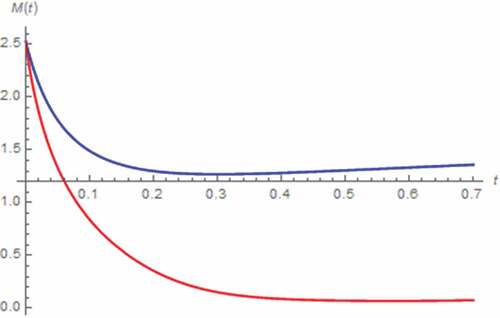
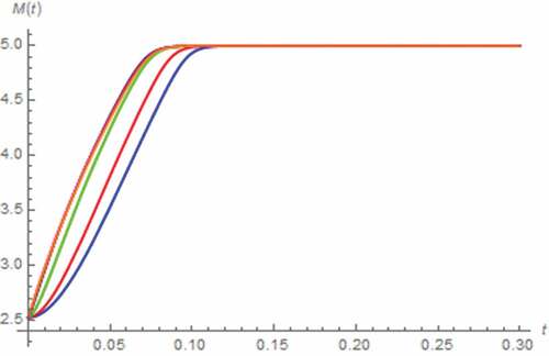
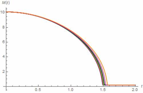
In order to perform the zero excitation-based analysis, we let v(t) = 0 V, x(0) = 0.5, y(0) = 0 C∙s^β−1, i(0) = 1 A. As a result, i(t) and M(t) assuming that the memristor is extended to fractional domain can be simulated as depicted in Figures 4–5 where the boundary effect induced saturation of memristor can be observed when α become fractional which implies that the saturation is occurred after the extension of memristor. Here, we have found that the extended device is saturated at M_on which implies that the device now contains only the region with high concentration of dopants i.e. doped region, (Strukov et al., 2008). The dynamic of i(t) assuming the fractional domain extended memristor is significantly different from that assuming the conventional one due to the saturation of the extended memristor which yields the linearity of the circuit (as M(t) is now fixed at M_on thus the memristor now behaves like a resistor), thus influences i(t). By further altering α, the time that it takes for the saturation to (t_sat), have been simulated as shown in Table 1 which shows that t_sat is directly proportional to α. It should be mentioned here that t_sat can be mathematically defined as M(t_sat) = M_on in this scenario. This is because the saturated value of M(t) is equal to M_on.

Table 1. t_sat vs. α (Nonlinear Series Circuit/Zero Excitation)

α	tsat(s)
0.10.30.50.70.9	2.6×10^−8sec0.000038sec0.0055sec0.05sec0.5 sec

Figure 4. I(t) vs. t (series circuit/zero excitation): α = 0.9 (red), α approaches 1 (blue)

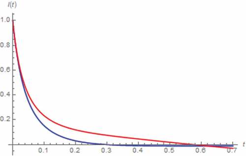
Figure 5. M(t) vs. t (series circuit/zero excitation): α = 0.9 (red), α approaches 1 (blue)

Now, we simulate i(t) and M(t) by assuming that the capacitor is extended to fractional domain. The results are depicted in Figures 6–7, which show that the saturation has occurred at M_off when β ≤ 0.7 and t_sat is directly proportional to β. Such saturation at M_off implies that the memristor now contains only the region with low concentration of dopants i.e. undoped region, (Strukov et al., 2008). It can be seen from Figure 7 that t_sat’s in this scenario are significantly longer than those tabulated in Table 1, and the highest value of β for obtaining the saturation is lower than that of α. Therefore, it can be stated that the extension of capacitor also affects the characteristic of memristor. However, a weaker effect than the extension of memristor itself can be observed. At this point, we perform the analysis based on the fractional domain extended inductor. As a result, we have found that such extension of inductor does not contribute the saturation. We have also found that the decaying rate of i(t) is inversely proportional to γ as can be seen from Figure 8.

Figure 6. I(t) vs. t (series circuit/zero excitation): β = 0.5 (black), β = 0.7 (green), β = 0.9 (red), β approaches 1 (blue)

Figure 7. M(t) vs. t (series circuit/zero excitation): β = 0.5 (black), β = 0.7 (green), β = 0.9 (red), β approaches 1 (blue)

Figure 8. I(t) vs. t (series circuit/zero excitation): γ = 0.7 (green), γ = 0.9 (red), γ approaches 1 (blue)

5.1.2. DC excitation

Here, we let v(t) = 5 V, x(0) = 0.5, y(0) = 0 C∙s^β−1, i(0) = 0 A. As a result, the simulated i(t) and M(t) assuming the fractional domain extended memristor are depicted in Figures 9–10, which show that the memristor can be saturated without the fractional domain extension at M_off, which in turn implies that the memristor now contains only the undoped region, and t_sat is directly proportional to α. By comparing Figure 9 with Table 1, we have found that longer t_sat is required in this scenario. The undershoot of i(t) which its magnitude is directly proportional to α, is ceased to be existed when α ≤ 0.5.

Figure 9. I(t) vs. t (series circuit/DC excitation): α = 0.1 (Orange), α = 0.3 (magenta), α = 0.5 (black), α = 0.7 (green), α = 0.9 (red), α approaches 1 (blue)

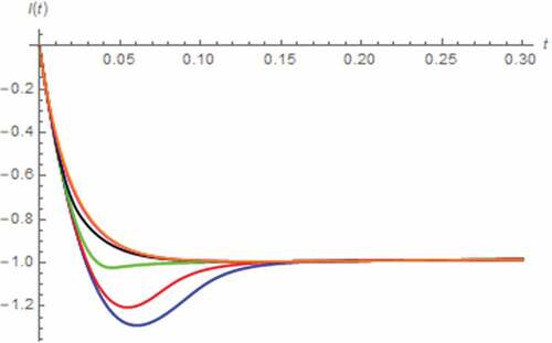
Figure 10. M(t) vs. t (series circuit/DC excitation): α = 0.1 (Orange), α = 0.3 (magenta), α = 0.5 (black), α = 0.7 (green), α = 0.9 (red), α approaches 1 (blue)

Now, we perform the simulation based on the fractional domain extended capacitor. It has been found that such extension of capacitor has insignificant effect on M(t) despite that it affects i(t) which controls the memristor, as can be seen from Figure 11. Finally, i(t) and M(t) simulated by assuming that the inductor is extended to fractional domain are depicted in Figures 12–13 where a saturation at M_off which implies the total domination of undoped region as stated above, can be observed. In addition, we have found that i(t) exhibits the undershoot which its magnitude and time of occurrence are respectively inversely and directly proportional to γ. The effect of γ on t_sat can be clearly seen when γ ≥ 0.7 where t_sat and nonlinearity of M(t) are directly proportional to γ. By the relationship between t_sat and γ, the circuit with higher γ can prolong its nonlinearity for longer period due to the longer unsaturated state of memristor. In summary, the extension of inductor affects the memristor and thus linearity of the entire circuit albeit a weaker effect than extending the memristor itself.

Figure 11. I(t) vs. t (series circuit/DC excitation): β = 0.1 (Orange), β = 0.3 (magenta), β = 0.5 (black), β = 0.7 (green), β = 0.9 (red), β approaches 1 (blue)

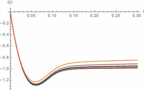
Figure 12. I(t) vs. t (series circuit/DC excitation): γ = 0.1 (Orange), γ = 0.3 (magenta), γ = 0.5 (black), γ = 0.7 (green), γ = 0.9 (red), γ approaches 1 (blue)

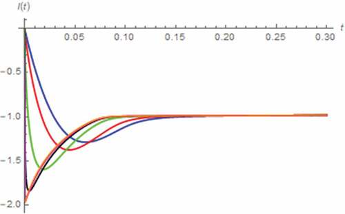
Figure 13. M(t) vs. t (series circuit/DC excitation): γ = 0.1 (Orange), γ = 0.3 (magenta), γ = 0.5 (black), γ = 0.7 (green), γ = 0.9 (red), γ approaches 1 (blue)

5.1.3. AC excitation

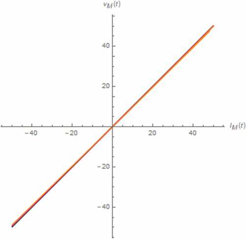
For performing the AC exciting signal-based analysis, v(t) = 5sin(30 t) V, x(0) = 0, y(0) = 0 C∙s^β−1 and i(0) = 0 have been assumed. As a result, i(t) and M(t) have been simulated by assuming the fractional domain extended memristor as depicted in Figures 14–15 where the voltage-current Lissajous patterns of the memristor have been simulated as depicted in Figures 16–17. Note that two figures are necessary for clarity. From these figures, we have found that a saturation occurred when α ≤ 0.7. The saturation is merely temporary because the drift of charge dopant is eventually resumed. When α < 0.3, the memristor can be respectively saturated at either M_on or M_off which implies the alternative total domination of doped and undoped regions, during the 1^st and 2^nd half cycles respectively. When α ≤ 0.3 ≤ 0.7 the memristor can be saturated at M_off only as only the total domination of undoped region can be occurred.

Figure 14. I(t) vs. t (series circuit/AC excitation): α = 0.1 (Orange), α = 0.3 (magenta), α = 0.5 (black), α = 0.7 (green), α = 0.9 (red), α approaches 1 (blue)

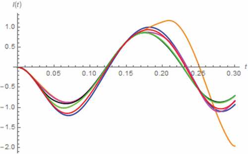
Figure 15. M(t) vs. t (series circuit/AC excitation): α = 0.1 (Orange), α = 0.3 (magenta), α = 0.5 (black), α = 0.7 (green), α = 0.9 (red), α approaches 1 (blue)

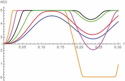
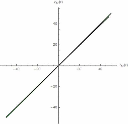
Figure 16. The v_M(t)-i_M(t) Lissajous patterns (series circuit): α = 0.1 (Orange), α = 0.3 (magenta), α = 0.5 (black)

Figure 17. The v_M(t)-i_M(t) Lissajous patterns (series circuit): α = 0.7 (green), α = 0.9 (red), α approaches 1 (blue)

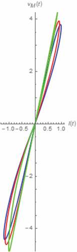
From the Lissajous patterns, we have found that the memristor’s signature of HP TiO₂ memristor is conserved by its fractional domain extension as these patterns take the pinched hysteresis loop shape despite asymmetrical shape and saturation induced distortion according to (Chua, 2014). By observing the lobe areas of these hysteresis loops, it has been found that the memristor employs more linearity thus providing less memory effect and circuit level nonlinearity with respected to α when v_M(t) and i_M(t) are their 1^st half cycles (and vice versa when v_M(t) and i_M(t) are their 2^nd half cycles) if α ≤ 0.5. If α > 0.5, the linearity of the memristor and thus the circuit for entire cycles of v_M(t) and i_M(t) is inversely proportional to α.

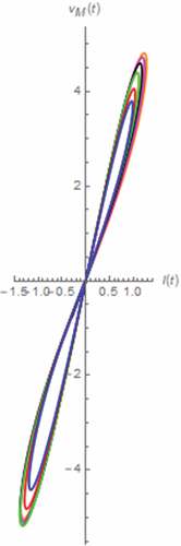
By respectively extending the capacitor and inductor to fractional domain, we have found that the saturation is not occurred unlike the above extension of memristor. From the simulated Lissajous patterns depicted in Figures 18–19, it has been found that such extension of reactive element conserves the abovementioned signature albeit affecting the memristor’s linearity. During the 1^st half cycle of v_M(t) and i_M(t), we have found that the linearity of the memristor and the entire circuit is inversely proportional to β. Such linearity is also inversely proportional to γ if γ < 0.7 and vice versa if 0.7 ≤ γ < 1. During the 2^nd half cycle on the other hand, the linearity become directly proportional to both β and γ. Note that the effect of extending the capacitor is insignificant compared to that of the inductor. However, the effect of the latter is weaker than the extension of memristor.

Figure 18. The v_M(t)-i_M(t) Lissajous patterns (series circuit): β = 0.1 (Orange), β = 0.3 (magenta), β = 0.5 (black), β = 0.7 (green), β = 0.9 (red), β approaches 1 (blue)

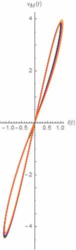
Figure 19. The v_M(t)-i_M(t) Lissajous patterns (series circuit): γ = 0.1 (Orange), γ = 0.3 (magenta), γ = 0.5 (black), γ = 0.7 (green), γ = 0.9 (red), γ approaches 1 (blue)

5.2. Nonlinear parallel circuit

For the parallel circuit which the solution of equation (18)(18) ${\mathrm{D}}^{\beta }[v(t)]=-\frac{v(t)}{[M_{on}x(t)+(1-x(t))M_{off}]C_{\beta }}-\frac{z(t)}{L_{\gamma }{C}_{\beta }}+\frac{i(t)}{C_{\beta }}$(18) must be adopted, we let M_on = 0.2 Ω, M_off = 20 Ω, L_γ = 0.3 H∙s^γ−1 and C_β = 10 F∙s^β−1 where k_α and p remain unchanged.

5.2.1. Zero excitation

Here, we have assumed that i(t) = 0 A, x(0) = 0.5, z(0) = 0 Wb∙s^γ−1, v(0) = 1 V. As a result, v(t) and M(t) assuming the fractional domain extended memristor can be simulated as depicted in Figures 20–21 where a saturation based on the total domination of undoped region has been occurred without the extension yet t_sat is directly proportional to α. Moreover, the inflection of v(t) caused by the saturation which alter the linearity of the circuit and thus v(t), can be observed. Such inflection is occurred sooner as α approaches 0 according to the relationship between t_sat and α. On the other hand, v(t) and M(t) can be simulated by assuming the fractional domain extended capacitor as depicted in Figures 22–23 where a saturation due to the total domination of undoped region can be observed. From both figures, it can be stated that the fractional domain extension of capacitor to also affects the memristor’s characteristic albeit with a weaker effect. Unlike the series circuit, we have found that t_sat is inversely proportional to β thus v(t) with lower β inflects later. These relationships with β of t_sat and v(t) become obvious when β ≤ 0.9.

Figure 20. V(t) vs. t (parallel circuit/zero input): α = 0.5 (black), α = 0.7 (green), α = 0.9 (red), α approaches 1 (blue)

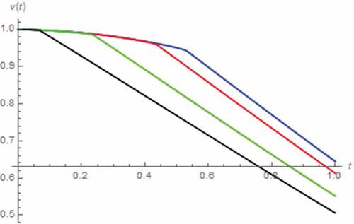
Figure 21. M(t) vs. t (parallel circuit/zero input): α = 0.5black), α = 0.7 (green), α = 0.9 (red), α approaches 1 (blue)

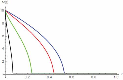
Figure 22. V(t) vs. t (parallel circuit/zero input): β = 0.1 (Orange), β = 0.3 (magenta), β = 0.5 (black), β = 0.7 (green), β = 0.9 (red), β approaches1 (blue)

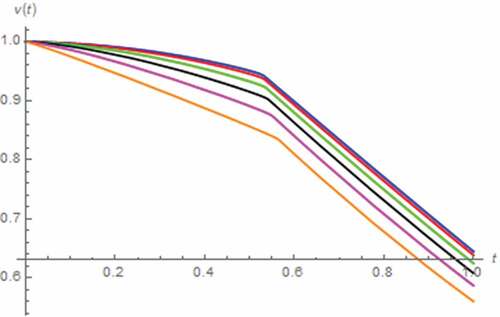
Figure 23. M(t) vs. t (parallel circuit/zero input): β = 0.1 (Orange), β = 0.3 (magenta), β = 0.5 (black), β = 0.7 (green), β = 0.9 (red), β approaches1 (blue)

Now, we perform the analysis by assuming the fractional domain extended inductor. The resulting v(t) and M(t) can be depicted in Figure 24–27. It has been found that the saturation due to the total domination of undoped region is occurred if γ ≤ 0.1 where t_sat is directly and proportional to γ. Otherwise, the saturation based on total domination of the doped region with t_sat be inversely proportional to γ is occurred and the saturation induced inflection of v(t), which become more obvious when γ approaches 1, can be observed. Note that the former t_sat is longer than the latter and the decreasing rate of v(t) is inversely proportional to γ whether γ ≤ 0.1 or not.

Figure 24. V(t) vs. t (parallel circuit/zero input): γ = 0.01 (dashed-blue), γ = 0.05 (dotted-blue), γ = 0.1 (Orange)

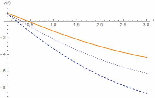
Figure 25. M(t) vs. t (parallel circuit/zero input): γ = 0.01 (dashed-blue), γ = 0.05 (dotted-blue), γ = 0.1 (Orange)

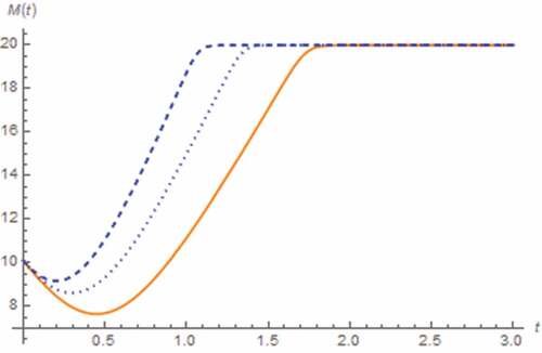
Figure 26. V(t) vs. t (parallel circuit/zero input): γ = 0.3 (magenta), γ = 0.5 (black), γ = 0.7 (green), γ = 0.9 (red), γ approaches 1 (blue)

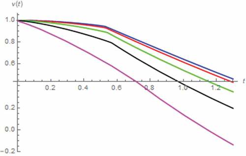
Figure 27. M(t) vs. t (parallel circuit/zero input): γ = 0.3 (magenta), γ = 0.5 (black), γ = 0.7 (green), γ = 0.9 (red), γ approaches 1 (blue)

5.2.2. DC excitation

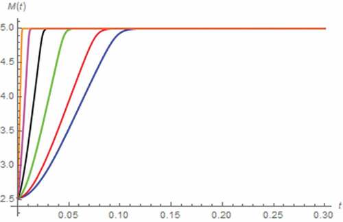
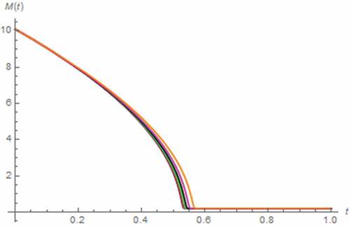
In this case, we assume that i(t) = 5 A, x(0) = 0.5, z(0) = 0 Wb∙s^γ−1, v(0) = 0 V. The resulting v(t) and M(t) simulated by assuming the fractional domain extended memristor can be depicted in Figures 28–29. Again, the saturation at M_on which refers to total domination of the doped region, can be occurred without the extension yet t_sat is directly proportional to α. The inflection of v(t) can also be observed where such inflection occurs sooner at lower α due to the relationship between t_sat and α. The effect of extending the memristor is obvious when α ≤ 0.7. By extending the capacitor to fractional domain on the other hand, the simulated v(t) and M(t) can be depicted in Figures 30–31, which show that the saturation is based on the total domination of doped region and t_sat is directly proportional to β. The inflection of v(t) which occurred sooner for lower β due to the relationship between t_sat and β, can be observed. From Figures 29–31, we have found that the fractional domain extension of capacitor is even more influential to the memristor than extending the memristor itself. At this point, we perform the analysis by assuming the extended inductor. The resulting v(t) and M(t) are depicted in Figures 32–33, which show that t_sat is inversely proportional to γ thus the inflection of v(t) occurs sooner for higher γ.

Figure 28. V(t) vs. t (parallel circuit/DC input): α = 0.1 (Orange), α = 0.3 (magenta), α = 0.5 (black), α = 0.7 (green), α = 0.9 (red), α approaches 1 (blue)

Figure 29. M(t) vs. t (parallel circuit/DC input): α = 0.1 (Orange), α = 0.3 (magenta), α = 0.5 (black), α = 0.7 (green), α = 0.9 (red), α approaches 1 (blue)

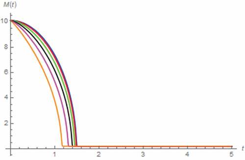
Figure 30. V(t) vs. t (parallel circuit/DC input): β = 0.5 (black), β = 0.7 (green), β = 0.9 (red), β approaches 1 (blue)

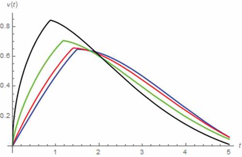
Figure 31. M(t) vs. t (parallel circuit/DC input): β = 0.5 (black), β = 0.7 (green), β = 0.9 (red), β approaches 1 (blue)

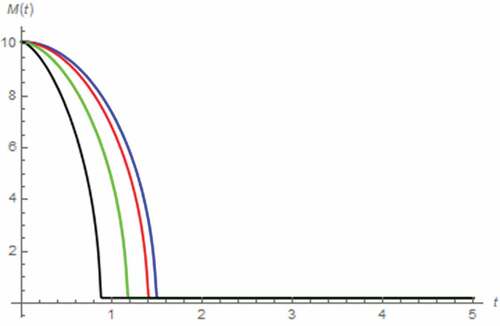
Figure 32. V(t) vs. t (parallel circuit/DC input): γ = 0.1 (Orange), γ = 0.3 (magenta), γ = 0.5 (black), γ = 0.7 (green), γ = 0.9 (red), γ approaches 1 (blue)

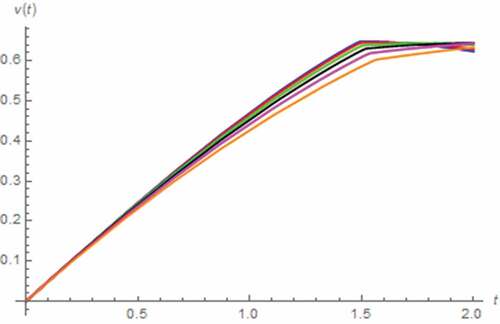
Figure 33. M(t) vs. t (parallel circuit/DC input): γ = 0.1 (Orange), γ = 0.3 (magenta) γ = 0.5 (black), γ = 0.7 (green), γ = 0.9 (red), γ approaches 1 (blue)

5.2.3. AC excitation

In order to perform the AC exciting signal-based analysis, we let i(t) = 5cos(30 t) A, x(0) = 0.5, z(0) = 0 Wb∙s^γ−1, v(0) = 0 V. As a result, v(t), M(t) and Lissajous pattern can be simulated by assuming the fractional domain extended memristor as depicted in Figures 34–36, which show that there exists no saturation. However, the nonlinearities of memristor and the entire circuit become very low. We have also found that the effect of such memristor extension is insignificant.

Figure 34. V(t) vs. t (parallel circuit/AC input): α = 0.1 (Orange), α = 0.3 (magenta), α = 0.5 (black), α = 0.7 (green), α = 0.9 (red), α approaches 1 (blue)

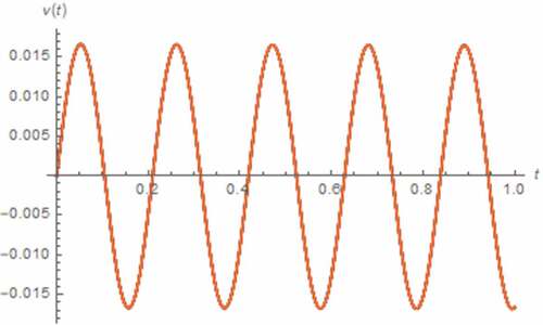
Figure 35. M(t) vs. t (parallel circuit/AC input): α = 0.1 (Orange), α = 0.3 (magenta), α = 0.5 (black), α = 0.7 (green), α = 0.9 (red), α approaches 1 (blue)

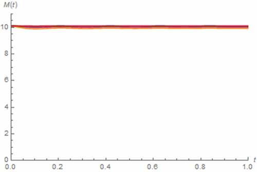
Figure 36. The v_M(t)-i_M(t) Lissajous patterns (parallel circuit): α = 0.1 (Orange), α = 0.3 (magenta), α = 0.5 (black), α = 0.7 (green), α = 0.9 (red), α approaches 1 (blue)

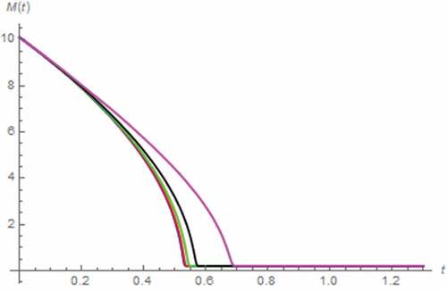
On the other hand, the effect of capacitor extension is significant. With β < 0.5, the simulated v(t), M(t) and Lissajous pattern can be depicted in Figures 37–39 where a permanent saturation at M_on can be observed. Such permanent saturation, which is based on the permanent total domination of the doped region due to the permanent inexistence of charge dopant drift, has begun at a certain instant that is directly proportional to β. In addition, the nonlinearity of the memristor and thus the circuit is inversely proportional to β as can be seen from the lobe areas of the Lissajous patterns. If we let 0.5 ≤ β < 1, the simulated results can be obtained as depicted in Figures 40–42 where we have found that there exists no saturation and the memristor is highly linear. The decreasing rate of M(t) and linearity of the entire circuit are inversely proportional to β. Whether β < 0.5 or not, we have found that the overall decreasing rate of v(t) is inversely proportional to β.

Figure 37. V(t) vs. t (parallel circuit/AC input): β = 0.1 (Orange), β = 0.3 (magenta)

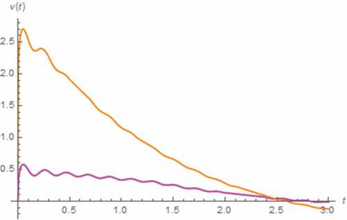
Figure 38. M(t) vs. t (parallel circuit/AC input): β = 0.1 (Orange), β = 0.3 (magenta)

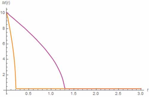
Figure 39. The v_M(t)-i_M(t) Lissajous patterns (parallel circuit): β = 0.1 (Orange), β = 0.3 (magenta)

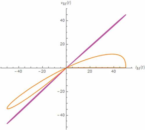
Figure 40. V(t) vs. t (parallel circuit/AC input): β = 0.5 (black), β = 0.7 (green), β = 0.9 (red), β approaches 1 (blue)

Figure 41. M(t) vs. t (parallel circuit/AC input): β = 0.5 (black), β = 0.7 (green), β = 0.9 (red), β approaches 1 (blue)

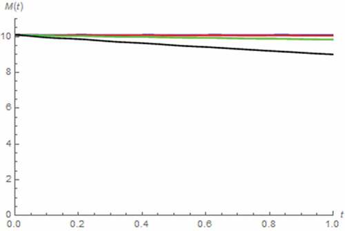
Figure 42. The v_M(t)-i_M(t) Lissajous patterns (parallel circuit): β = 0.5 (black), β = 0.7 (green), β = 0.9 (red), β approaches 1 (blue)

Finally, we perform the analysis by assuming the fractional domain extended inductor. The results can be simulated as depicted in Figures 43–45 where we have found that the memristor always be saturated at M_off due to the permanent domination of undoped region. The effect of inductor extension on the entire circuit is significant. The circuit’s linearity is directly proportional to γ as more distorted v(t) with lower γ can be observed.

Figure 43. V(t) vs. t (parallel circuit/AC input): γ = 0.1 (Orange), γ = 0.3 (magenta), γ = 0.5 (black), γ = 0.7 (green), γ = 0.9 (red), γ approaches 1 (blue)

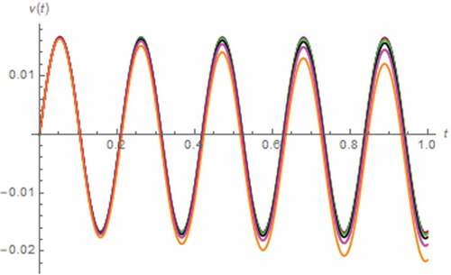
Figure 44. M(t) vs. t (parallel circuit/AC input): γ = 0.1 (Orange), γ = 0.3 (magenta), γ = 0.5 (black), γ = 0.7 (green), γ = 0.9 (red), γ approaches 1 (blue)

Figure 45. The v_M(t)-i_M(t) Lissajous patterns (parallel circuit): γ = 0.1 (Orange), γ = 0.3 (magenta), γ = 0.5 (black), γ = 0.7 (green), γ = 0.9 (red), γ approaches 1 (blue)

6. Discussion

In the previous section, we have found that the fractional domain extension of capacitor also affects the characteristic of memristor. For the series circuit, this is because such extension affects i(t) which in turn controls the memristor, as can be seen from Figure 6. For the parallel circuit, the reason is that the extension of capacitor affects v(t) which in turn affects i_M(t) that controls the memristor. On the other hand, we have found that the fractional domain extension of inductor also affects the memristor and thus linearity of the entire circuit as well. This is because such extension affects i(t) and the memristor is current controlled. In addition, we have found that the decaying rates of i(t) of the series circuit and v(t) of the parallel circuit are inversely proportional to γ. This is not surprising because 0 < γ < 1, t ≤ 1 and $\frac{\mathrm{d}i(t)}{\mathrm{d}t}\begin{array}{c}\hspace{0.17em}\end{array}\propto \begin{array}{c}\hspace{0.17em}\end{array}{t}^{\gamma -1}$ as can be seen from the 3^rd line of equation (11)(11) $\frac{\mathrm{d}y(t)}{\mathrm{d}t}=t^{\beta -1}i(t)$(11) . On the other hand, it can be seen from the 2^nd line of equation (19)(19) $\frac{\mathrm{d}v(t)}{\mathrm{d}t}=-\frac{t^{\beta -1}v(t)}{[M_{on}x(t)+(1-x(t))M_{off}]C_{\beta }}-\frac{t^{\beta -1}}{L_{\gamma }{C}_{\beta }}z(t)+\frac{t^{\beta -1}}{C_{\beta }}i(t)$(19) that $\frac{\mathrm{d}v(t)}{\mathrm{d}t}\begin{array}{c}\hspace{0.17em}\end{array}\propto \begin{array}{c}\hspace{0.17em}\end{array}z(t)$where of z(t) is inversely proportional to γ because the by part integration of the 3^rd line of equation (19)(19) $\frac{\mathrm{d}v(t)}{\mathrm{d}t}=-\frac{t^{\beta -1}v(t)}{[M_{on}x(t)+(1-x(t))M_{off}]C_{\beta }}-\frac{t^{\beta -1}}{L_{\gamma }{C}_{\beta }}z(t)+\frac{t^{\beta -1}}{C_{\beta }}i(t)$(19) gives $z(t)=\frac{1}{\gamma }[t^{\gamma }v(t)-\underset{v(0)}{\overset{v(t)}{\int }}{\tau }^{\gamma }dv(\tau )]$.

Since the most important observation from the simulation results is the stability of both HP TiO₂ memristor-based nonlinear circuits, the stability of these circuits will be now mathematically verified. Firstly, the series circuit will be considered. Under the zero input and AC input with t = nπ where {n} = {0, 1, 2, … }, equation (10)(10) ${\mathrm{D}}^{\beta }[y(t)]=i(t)$(10) become

${\mathrm{D}}^{\alpha }[x(t)]=k_{\alpha }i(t)(1-(2x(t)-1{)}^{2p})$

(24) ${\mathrm{D}}^{\beta }[y(t)]=i(t)$(24)

${\mathrm{D}}^{\gamma }[i(t)]=-(M_{on}x(t)+(1-x(t))M_{off})L_{\gamma }^{-1}i(t)-C_{\beta }^{-1}{L}_{\gamma }^{-1}y(t)$

On the other hand, the following nonlinear FDEs can be obtained if the DC input has been applied

${\mathrm{D}}^{\alpha }[x(t)]=k_{\alpha }i(t)(1-(2x(t)-1{)}^{2p})$

(25) ${\mathrm{D}}^{\beta }[y(t)]=i(t)$(25)

${\mathrm{D}}^{\gamma }[i(t)]=-(M_{on}x(t)+(1-x(t))M_{off})L_{\gamma }^{-1}i(t)-C_{\beta }^{-1}{L}_{\gamma }^{-1}y(t)+L_{\gamma }^{-1}V$

As a result, the set of equilibrium points of equations (24)(24) ${\mathrm{D}}^{\beta }[y(t)]=i(t)$(24) and (25(25) ${\mathrm{D}}^{\beta }[y(t)]=i(t)$(25) ) can be, respectively, found as E₀ = (χ, 0, 0) and E_DC = (χ, C_βV, 0) where χ refers to the value of x(t) at each equilibrium point. Therefore, the associated Jacobian matrices can be obtained as follows

(26) ${\mathbf{J}}_{{\mathbf{E}}_0}={\mathbf{J}}_{{\mathbf{E}}_{DC}}=\left[\begin{array}{ccc}0& 0& k_{\delta }i(1-{(2\chi -1)}^{2p})\\ 0& 0& 1\\ 0& -L_{\delta }^{-1}{C}_{\delta }^{-1}& -(M_{on}\chi +(1-\chi )M_{off})L_{\delta }^{-1}\end{array}\right]$(26)

where α = β = γ = δ has been assumed for simplicity.

By using equation (26)(26) ${\mathbf{J}}_{{\mathbf{E}}_0}={\mathbf{J}}_{{\mathbf{E}}_{DC}}=\left[\begin{array}{ccc}0& 0& k_{\delta }i(1-{(2\chi -1)}^{2p})\\ 0& 0& 1\\ 0& -L_{\delta }^{-1}{C}_{\delta }^{-1}& -(M_{on}\chi +(1-\chi )M_{off})L_{\delta }^{-1}\end{array}\right]$(26) , the following characteristic equation can be obtained

(27) ${\lambda }^3+(M_{on}\chi +(1-\chi )M_{off})L_{\delta }^{-1}{\lambda }^2+L_{\delta }^{-1}{C}_{\delta }^{-1}\lambda =0$(27)

which yields ${\lambda }_1=0$ and ${\lambda }_{2,3}=-\frac{M_{off}-(M_{off}-M_{on})\chi }{2L_{\delta }^{\hspace{0.17em}}}\pm j\frac{\sqrt{4L_{\delta }^{\hspace{0.17em}}{C}_{\delta }^{\hspace{0.17em}}-C_{\delta }^2{(M_{off}-(M_{off}-M_{on})\chi )}^2}}{2L_{\delta }^{\hspace{0.17em}}{C}_{\delta }^{\hspace{0.17em}}}$.

In the integer domain, the instability occurs if at least either λ₂ or λ₃ reside in the right half of the complex plane which means that

(28) $\chi >\frac{1}{1-\frac{M_{on}}{M_{off}}}$(28)

must be satisfied.

By extending to the fractional domain, such right half plane maps into a wedge shape with angle of δπ/2 (Cafagna & Grassi, 2012). As a result, the additional condition on δ i.e., $\frac{\delta \pi }{2}>\left|{tan}^{-1}[\frac{Im[{\lambda }_{2,3}]}{Re[{\lambda }_{2,3}]}]\right|$, must be satisfied. By applying the above ${\lambda }_{2,3}$, this condition can be given by

(29) $\frac{\delta \pi }{2}>\left|{tan}^{-1}[\mp \frac{\sqrt{4L_{\delta }^{\hspace{0.17em}}{C}_{\delta }^{\hspace{0.17em}}-C_{\delta }^2{(M_{off}-(M_{off}-M_{on})\chi )}^2}}{C_{\delta }^{\hspace{0.17em}}(M_{off}-(M_{off}-M_{on})\chi )}]\right|$(29)

For more detailed study, we firstly assume that only the memristor is extended to fractional domain. Therefore, we now have β = γ = 1. Since the orders of the FDEs become incommensurate, it is more appropriated to rely on the complex frequency termed characteristic equation as did by Deng (Deng et al., 2007) instead of the Eigen value termed one like equation (27)(27) ${\lambda }^3+(M_{on}\chi +(1-\chi )M_{off})L_{\delta }^{-1}{\lambda }^2+L_{\delta }^{-1}{C}_{\delta }^{-1}\lambda =0$(27) . Based on equation (26)(26) ${\mathbf{J}}_{{\mathbf{E}}_0}={\mathbf{J}}_{{\mathbf{E}}_{DC}}=\left[\begin{array}{ccc}0& 0& k_{\delta }i(1-{(2\chi -1)}^{2p})\\ 0& 0& 1\\ 0& -L_{\delta }^{-1}{C}_{\delta }^{-1}& -(M_{on}\chi +(1-\chi )M_{off})L_{\delta }^{-1}\end{array}\right]$(26) , such complex frequency termed characteristic equation can be given by

(30) $s^{2+\delta }+(M_{on}\chi +(1-\chi )M_{off})L_{\delta }^{-1}{s}^{1+\delta }+L_{\delta }^{-1}{C}_{\delta }^{-1}{s}^{\delta }=0$(30)

After solving equation (30)(30) $s^{2+\delta }+(M_{on}\chi +(1-\chi )M_{off})L_{\delta }^{-1}{s}^{1+\delta }+L_{\delta }^{-1}{C}_{\delta }^{-1}{s}^{\delta }=0$(30) , we have found that $s_1=0$ and $s_{2,3}=-\frac{M_{off}-(M_{off}-M_{on})\chi }{2L_{\delta }^{\hspace{0.17em}}}\pm j\frac{\sqrt{4L_{\delta }^{\hspace{0.17em}}{C}_{\delta }^{\hspace{0.17em}}-C_{\delta }^2{(M_{off}-(M_{off}-M_{on})\chi )}^2}}{2L_{\delta }^{\hspace{0.17em}}{C}_{\delta }^{\hspace{0.17em}}}$. According to (Deng et al., 2007), the instability occurs if at least either s₂ or s₃ reside in the right half of the s-plane, which implies that equation (28)(28) $\chi >\frac{1}{1-\frac{M_{on}}{M_{off}}}$(28) must be satisfied.

Now, we assume that only the reactive elements are extended to fractional domain. Thus, we have α = 1. In this scenario, the following complex frequency termed characteristic equation can be obtained

(31) $s^{1+2\delta }+(M_{on}\chi +(1-\chi )M_{off})L_{\delta }^{-1}{s}^{1+\delta }+L_{\delta }^{-1}{C}_{\delta }^{-1}s=0$(31)

By solving equation (31)(31) $s^{1+2\delta }+(M_{on}\chi +(1-\chi )M_{off})L_{\delta }^{-1}{s}^{1+\delta }+L_{\delta }^{-1}{C}_{\delta }^{-1}s=0$(31) , we have found that $s_1=0$ and$s_{2,3}=\left[-\frac{M_{off}-(M_{off}-M_{on})\chi }{2L_{\delta }^{\hspace{0.17em}}}\right.{\left.\pm j\frac{\sqrt{4L_{\delta }^{\hspace{0.17em}}{C}_{\delta }^{\hspace{0.17em}}-C_{\delta }^2{(M_{off}-(M_{off}-M_{on})\chi )}^2}}{2L_{\delta }^{\hspace{0.17em}}{C}_{\delta }^{\hspace{0.17em}}}\right]}^{\frac{1}{\delta }}$

where the latter root yields

(32) $\mathrm{A}\mathrm{r}\mathrm{g}[s_{2.3}]=\frac{1}{\delta }{tan}^{-1}[\mp \frac{\sqrt{4L_{\delta }^{\hspace{0.17em}}{C}_{\delta }^{\hspace{0.17em}}-C_{\delta }^2{(M_{off}-(M_{off}-M_{on})\chi )}^2}}{C_{\delta }^{\hspace{0.17em}}(M_{off}-(M_{off}-M_{on})\chi )}]$(32)

For s_2,3 be in the right half of the s-plane, $\left|\mathrm{A}\mathrm{r}\mathrm{g}[s_{2.3}]\right|>\pi /2$ must be satisfied (Deng et al., 2007) which is equivalent to satisfying equation (29)(29) $\frac{\delta \pi }{2}>\left|{tan}^{-1}[\mp \frac{\sqrt{4L_{\delta }^{\hspace{0.17em}}{C}_{\delta }^{\hspace{0.17em}}-C_{\delta }^2{(M_{off}-(M_{off}-M_{on})\chi )}^2}}{C_{\delta }^{\hspace{0.17em}}(M_{off}-(M_{off}-M_{on})\chi )}]\right|$(29) . At this point, it has been found that the additional condition on δ is imposed by extending inductor and capacitor to the fractional domain.

If the AC input with t ≠ nπ has been applied, equation (10)(10) ${\mathrm{D}}^{\beta }[y(t)]=i(t)$(10) become

${\mathrm{D}}^{\alpha }[x(t)]=k_{\alpha }i(t)(1-(2x(t)-1{)}^{2p})$

(33) ${\mathrm{D}}^{\beta }[y(t)]=i(t)$(33)

${\mathrm{D}}^{\gamma }[i(t)]=-(M_{on}x(t)+(1-x(t))M_{off})L_{\gamma }^{-1}i(t)-C_{\beta }^{-1}{L}_{\gamma }^{-1}y(t)+L_{\gamma }^{-1}{v}_{AC}(t)$

where v_AC(t) stands for the instantaneous value of applied AC voltage with the frequency and peak value of ω and V. Note also that v_AC(t) ≠ 0 thus equation (33)(33) ${\mathrm{D}}^{\beta }[y(t)]=i(t)$(33) is non-autonomous.

By introducing an additional state variable namely τ(t) = t, and keeping in mind that the fractional derivative terms are the fractional conformable derivatives, equation (33)(33) ${\mathrm{D}}^{\beta }[y(t)]=i(t)$(33) become

${\mathrm{D}}^{\alpha }[x(t)]=k_{\alpha }i(t)(1-(2x(t)-1{)}^{2p})$

(34) ${\mathrm{D}}^{\beta }[y(t)]=i(t)$(34)

${\mathrm{D}}^{\gamma }[i(t)]=-(M_{on}x(t)+(1-x(t))M_{off})L_{\gamma }^{-1}i(t)-C_{\beta }^{-1}{L}_{\gamma }^{-1}y(t)+L_{\gamma }^{-1}{v}_{AC}(\tau (t))$

${\mathrm{D}}^{\delta }[\tau (t)]=(\tau (t){)}^{1-\delta }$

which is autonomous and employs E = (χ, 0, 0, 0) as its set of equilibrium points. Noted that E ceased to be existed in the integer domain.

Thus, the Jacobian matrix of equation (34)(34) ${\mathrm{D}}^{\beta }[y(t)]=i(t)$(34) at E can be found as

(35) ${\mathbf{J}}_{\mathbf{E}}=\left[\begin{array}{cccc}0& 0& k_{\delta }(1-{(2\chi -1)}^{2p})& 0\\ 0& 0& 1& 0\\ 0& -L_{\delta }^{-1}{C}_{\delta }^{-1}& -(M_{on}\chi +(1-\chi )M_{off})L_{\delta }^{-1}& \omega V{L}_{\delta }^{-1}\\ 0& 0& 0& 0\end{array}\right]$(35)

where α = β = γ = δ has been assumed for simplicity.

As a result, the following characteristic equation can be obtained

(36) ${\lambda }^4+(M_{on}\chi +(1-\chi )M_{off})L_{\delta }^{-1}{\lambda }^3+L_{\delta }^{-1}{C}_{\delta }^{-1}{\lambda }^2=0$(36)

After solving equation (36)(36) ${\lambda }^4+(M_{on}\chi +(1-\chi )M_{off})L_{\delta }^{-1}{\lambda }^3+L_{\delta }^{-1}{C}_{\delta }^{-1}{\lambda }^2=0$(36) , we have ${\lambda }_1=0$, ${\lambda }_2=0$ and

${\lambda }_{3,4}=-\frac{M_{off}-(M_{off}-M_{on})\chi }{2L_{\delta }^{\hspace{0.17em}}}\pm j\frac{\sqrt{4L_{\delta }^{\hspace{0.17em}}{C}_{\delta }^{\hspace{0.17em}}-C_{\delta }^2{(M_{off}-(M_{off}-M_{on}\chi ))}^2}}{2L_{\delta }^{\hspace{0.17em}}{C}_{\delta }^{\hspace{0.17em}}}$. In the integer domain, the instability occur if λ_3,4 reside in the right half of the complex plane which means that equation (28)(28) $\chi >\frac{1}{1-\frac{M_{on}}{M_{off}}}$(28) must be satisfied. By the extension to fractional domain, the additional condition on δ i.e., $\frac{\delta \pi }{2}>\left|{tan}^{-1}[\frac{Im[{\lambda }_{3,4}]}{Re[{\lambda }_{3,4}]}]\right|$, which is equivalent to equation (29)(29) $\frac{\delta \pi }{2}>\left|{tan}^{-1}[\mp \frac{\sqrt{4L_{\delta }^{\hspace{0.17em}}{C}_{\delta }^{\hspace{0.17em}}-C_{\delta }^2{(M_{off}-(M_{off}-M_{on})\chi )}^2}}{C_{\delta }^{\hspace{0.17em}}(M_{off}-(M_{off}-M_{on})\chi )}]\right|$(29) , must be satisfied.

If we now extend only the memristor to fractional domain, the resulting s-domain characteristic equation can be obtained by using equation (35)(35) ${\mathbf{J}}_{\mathbf{E}}=\left[\begin{array}{cccc}0& 0& k_{\delta }(1-{(2\chi -1)}^{2p})& 0\\ 0& 0& 1& 0\\ 0& -L_{\delta }^{-1}{C}_{\delta }^{-1}& -(M_{on}\chi +(1-\chi )M_{off})L_{\delta }^{-1}& \omega V{L}_{\delta }^{-1}\\ 0& 0& 0& 0\end{array}\right]$(35) as follows

(37) $s^{2+2\delta }+(M_{on}\chi +(1-\chi )M_{off})L_{\delta }^{-1}{s}^{1+2\delta }+L_{\delta }^{-1}{C}_{\delta }^{-1}{s}^{2\delta }=0$(37)

After solving (37), we have found that $s_1=0$, $s_2=0$ and

$s_{3,4}=-\frac{M_{off}-(M_{off}-M_{on})\chi }{2L_{\delta }^{\hspace{0.17em}}}\pm j\frac{\sqrt{4L_{\delta }^{\hspace{0.17em}}{C}_{\delta }^{\hspace{0.17em}}-C_{\delta }^2{(M_{off}-(M_{off}-M_{on})\chi )}^2}}{2L_{\delta }^{\hspace{0.17em}}{C}_{\delta }^{\hspace{0.17em}}}$which shows that an instability occurs if at least either s₃ or s₄ reside in the right half of the s-plane thus equation (28)(28) $\chi >\frac{1}{1-\frac{M_{on}}{M_{off}}}$(28) must be satisfied.

At this point, we extend only the reactive elements. Therefore, the following characteristic equation can be obtained

(38) $s^{1+3\delta }+(M_{on}\chi +(1-\chi )M_{off})L_{\delta }^{-1}{s}^{1+2\delta }+L_{\delta }^{-1}{C}_{\delta }^{-1}{s}^{1+\delta }=0$(38)

As a result, we have found that $s_1=0$, $s_2=0$ and

$s_{3,4}=\left[-\frac{M_{off}-(M_{off}-M_{on})\chi }{2L_{\delta }^{\hspace{0.17em}}}\right.{\left.\pm j\frac{\sqrt{4L_{\delta }^{\hspace{0.17em}}{C}_{\delta }^{\hspace{0.17em}}-C_{\delta }^2{(M_{off}-(M_{off}-M_{on})\chi )}^2}}{2L_{\delta }^{\hspace{0.17em}}{C}_{\delta }^{\hspace{0.17em}}}\right]}^{\frac{1}{\delta }}$. It can be seen from s_3,4 that

(39) $\mathrm{A}\mathrm{r}\mathrm{g}[s_{3,4}]=\frac{1}{\delta }{tan}^{-1}[\mp \frac{\sqrt{4L_{\delta }^{\hspace{0.17em}}{C}_{\delta }^{\hspace{0.17em}}-C_{\delta }^2{(M_{off}-(M_{off}-M_{on})\chi )}^2}}{C_{\delta }^{\hspace{0.17em}}(M_{off}-(M_{off}-M_{on})\chi )}]$(39)

For obtaining the instability $\left|\mathrm{A}\mathrm{r}\mathrm{g}[s_{3,4}]\right|>\pi /2$ must be satisfied which is equivalent to satisfying equation (29)(29) $\frac{\delta \pi }{2}>\left|{tan}^{-1}[\mp \frac{\sqrt{4L_{\delta }^{\hspace{0.17em}}{C}_{\delta }^{\hspace{0.17em}}-C_{\delta }^2{(M_{off}-(M_{off}-M_{on})\chi )}^2}}{C_{\delta }^{\hspace{0.17em}}(M_{off}-(M_{off}-M_{on})\chi )}]\right|$(29) . Here, it has been found that the additional condition on δ is imposed by extending both reactive elements to the fractional domain.

Now, consider the parallel circuit. Under the zero input and AC input with t = (n + 0.5)π where {n} = {0, 1, 2, … }, equation (18)(18) ${\mathrm{D}}^{\beta }[v(t)]=-\frac{v(t)}{[M_{on}x(t)+(1-x(t))M_{off}]C_{\beta }}-\frac{z(t)}{L_{\gamma }{C}_{\beta }}+\frac{i(t)}{C_{\beta }}$(18) become

${\mathrm{D}}^{\alpha }[x(t)]=\frac{k_{\alpha }v(t)(1-{(2x(t)-1)}^{2p})}{M_{on}x(t)+(1-x(t))M_{off}}$

(40) ${\mathrm{D}}^{\beta }[v(t)]=-\frac{v(t)}{[M_{on}x(t)+(1-x(t))M_{off}]C_{\beta }}-\frac{z(t)}{L_{\gamma }{C}_{\beta }}$(40)

${\mathrm{D}}^{\gamma }[z(t)]=v(t)$

If the DC input has been applied, we have

${\mathrm{D}}^{\alpha }[x(t)]=\frac{k_{\alpha }v(t)(1-{(2x(t)-1)}^{2p})}{M_{on}x(t)+(1-x(t))M_{off}}$

(41) ${\mathrm{D}}^{\beta }[v(t)]=-\frac{v(t)}{[M_{on}x(t)+(1-x(t))M_{off}]C_{\beta }}-\frac{z(t)}{L_{\gamma }{C}_{\beta }}+\frac{I}{C_{\beta }}$(41)

${\mathrm{D}}^{\gamma }[z(t)]=v(t)$

The set of equilibrium points of equations (40)(40) ${\mathrm{D}}^{\beta }[v(t)]=-\frac{v(t)}{[M_{on}x(t)+(1-x(t))M_{off}]C_{\beta }}-\frac{z(t)}{L_{\gamma }{C}_{\beta }}$(40) and (41(41) ${\mathrm{D}}^{\beta }[v(t)]=-\frac{v(t)}{[M_{on}x(t)+(1-x(t))M_{off}]C_{\beta }}-\frac{z(t)}{L_{\gamma }{C}_{\beta }}+\frac{I}{C_{\beta }}$(41) ) can be respectively found as E₀ = (χ, 0, 0) and E_DC = (χ, 0, L_γI). As a result, Jacobian matrices of these equations at E₀ and E_DC can be obtained as follows

(42) ${\mathbf{J}}_{{\mathbf{E}}_0}={\mathbf{J}}_{{\mathbf{E}}_{DC}}=\left[\begin{array}{ccc}0& 0& \frac{k_{\delta }i(1-{(2\chi -1)}^{2p})}{M_{on}\chi +(1-\chi )M_{off}}\\ 0& -C_{\delta }^{-1}{(M_{on}\chi +(1-\chi )M_{off})}^{-1}& -L_{\delta }^{-1}{C}_{\delta }^{-1}\\ 0& 1& 0\end{array}\right]$(42)

where α = β = γ = δ has also been assumed for simplicity.

As a result, the following characteristic equation can be obtained

(43) ${\lambda }^3+(M_{on}\chi -(1+\chi )M_{off}{)}^{-1}{C}_{\delta }^{-1}{\lambda }^2+L_{\delta }^{-1}{C}_{\delta }^{-1}\lambda =0$(43)

which yields${\lambda }_1=0$ and

${\lambda }_{2,3}=-\frac{1}{2C_{\delta }^{\hspace{0.17em}}(M_{off}-(M_{off}-M_{on})\chi )}\pm j\frac{\sqrt{4L_{\delta }^{\hspace{0.17em}}{C}_{\delta }^{\hspace{0.17em}}{(M_{off}-(M_{off}-M_{on})\chi )}^2-L_{\delta }^2}}{2L_{\delta }^{\hspace{0.17em}}{C}_{\delta }^{\hspace{0.17em}}(M_{off}-(M_{off}-M_{on})\chi )}$

.

In the integer domain, λ_2,3 must reside in the right half of the complex plane for the circuit become unstable thus equation (28)(28) $\chi >\frac{1}{1-\frac{M_{on}}{M_{off}}}$(28) must be satisfied. By the extension to fractional domain, the following additional condition on δ which can be obtained in a similar manner to equation (29)(29) $\frac{\delta \pi }{2}>\left|{tan}^{-1}[\mp \frac{\sqrt{4L_{\delta }^{\hspace{0.17em}}{C}_{\delta }^{\hspace{0.17em}}-C_{\delta }^2{(M_{off}-(M_{off}-M_{on})\chi )}^2}}{C_{\delta }^{\hspace{0.17em}}(M_{off}-(M_{off}-M_{on})\chi )}]\right|$(29) , must also be satisfied.

(44) $\frac{\delta \pi }{2}>\left|{tan}^{-1}[\mp \frac{\sqrt{4L_{\delta }^{\hspace{0.17em}}{C}_{\delta }^{\hspace{0.17em}}{(M_{off}-(M_{off}-M_{on})\chi )}^2-L_{\delta }^2}}{L_{\delta }^{\hspace{0.17em}}}]\right|$(44)

If we extend only the memristor, the following complex frequency termed characteristic equation can be obtained

(45) $s^{2+\delta }+(M_{on}\chi -(1+\chi )M_{off})C_{\delta }^{-1}{s}^{1+\delta }+L_{\delta }^{-1}{C}_{\delta }^{-1}{s}^{\delta }=0$(45)

By solving (45), we have $s_1=0$ and

$s_{2,3}=-\frac{1}{2C_{\delta }^{\hspace{0.17em}}(M_{off}-(M_{off}-M_{on})\chi )}\pm j\frac{\sqrt{4L_{\delta }^{\hspace{0.17em}}{C}_{\delta }^{\hspace{0.17em}}{(M_{off}-(M_{off}-M_{on})\chi )}^2+L_{\delta }^2}}{2L_{\delta }^{\hspace{0.17em}}{C}_{\delta }^{\hspace{0.17em}}(M_{off}-(M_{off}-M_{on})\chi )}$

.

Since the instability occurs if at least either s₂ or s₃ reside in the right half of the s-plane, equation (28)(28) $\chi >\frac{1}{1-\frac{M_{on}}{M_{off}}}$(28) must be satisfied. If we now extend only the reactive elements, we have

(46) $s^{1+2\delta }+(M_{on}\chi -(1+\chi )M_{off})C_{\delta }^{-1}{s}^{1+\delta }+L_{\delta }^{-1}{C}_{\delta }^{-1}s=0$(46)

By solving equation (46)(46) $s^{1+2\delta }+(M_{on}\chi -(1+\chi )M_{off})C_{\delta }^{-1}{s}^{1+\delta }+L_{\delta }^{-1}{C}_{\delta }^{-1}s=0$(46) , we have found that $s_1=0$ and

$s_{2,3}=\left[-\frac{1}{2C_{\delta }^{\hspace{0.17em}}(M_{off}-(M_{off}-M_{on})\chi )}\right.{\left.\pm j\frac{\sqrt{4L_{\delta }^{\hspace{0.17em}}{C}_{\delta }^{\hspace{0.17em}}{(M_{off}-(M_{off}-M_{on})\chi )}^2-L_{\delta }^2}}{2L_{\delta }^{\hspace{0.17em}}{C}_{\delta }^{\hspace{0.17em}}(M_{off}-(M_{off}-M_{on})\chi )}\right]}^{\frac{1}{\delta }}$

.

Thus, we have

(47) $\mathrm{A}\mathrm{r}\mathrm{g}[s_{2.3}]=\frac{1}{\delta }{tan}^{-1}[\mp \frac{\sqrt{4L_{\delta }^{\hspace{0.17em}}{C}_{\delta }^{\hspace{0.17em}}{(M_{off}-(M_{off}-M_{on})\chi )}^2-L_{\delta }^2}}{L_{\delta }}]$(47)

For obtaining $\left|\mathrm{A}\mathrm{r}\mathrm{g}[s_{2.3}]\right|>\pi /2$ which implies instability, equation (47)(47) $\mathrm{A}\mathrm{r}\mathrm{g}[s_{2.3}]=\frac{1}{\delta }{tan}^{-1}[\mp \frac{\sqrt{4L_{\delta }^{\hspace{0.17em}}{C}_{\delta }^{\hspace{0.17em}}{(M_{off}-(M_{off}-M_{on})\chi )}^2-L_{\delta }^2}}{L_{\delta }}]$(47) shows that equation (44)(44) $\frac{\delta \pi }{2}>\left|{tan}^{-1}[\mp \frac{\sqrt{4L_{\delta }^{\hspace{0.17em}}{C}_{\delta }^{\hspace{0.17em}}{(M_{off}-(M_{off}-M_{on})\chi )}^2-L_{\delta }^2}}{L_{\delta }^{\hspace{0.17em}}}]\right|$(44) must be satisfied thus it can be seen that the additional condition on δ has been imposed by the fractional domain extensions of both reactive elements.

If the AC input with t ≠ (n + 0.5)π has been applied, equation (18)(18) ${\mathrm{D}}^{\beta }[v(t)]=-\frac{v(t)}{[M_{on}x(t)+(1-x(t))M_{off}]C_{\beta }}-\frac{z(t)}{L_{\gamma }{C}_{\beta }}+\frac{i(t)}{C_{\beta }}$(18) become

${\mathrm{D}}^{\alpha }[x(t)]=\frac{k_{\alpha }v(t)(1-{(2x(t)-1)}^{2p})}{M_{on}x(t)+(1-x(t))M_{off}}$

(48) ${\mathrm{D}}^{\beta }[v(t)]=-\frac{v(t)}{[M_{on}x(t)+(1-x(t))M_{off}]C_{\beta }}-\frac{z(t)}{L_{\gamma }{C}_{\beta }}+\frac{i_{AC}(t)}{C_{\beta }}$(48)

${\mathrm{D}}^{\gamma }[z(t)]=v(t)$

where i_AC(t) stands for the instantaneous value of applied AC current with peak value ofIand frequency of ω. Note also that i_AC(t) ≠ 0 thus equation (48)(48) ${\mathrm{D}}^{\beta }[v(t)]=-\frac{v(t)}{[M_{on}x(t)+(1-x(t))M_{off}]C_{\beta }}-\frac{z(t)}{L_{\gamma }{C}_{\beta }}+\frac{i_{AC}(t)}{C_{\beta }}$(48) is non-autonomous similar to equation (33)(33) ${\mathrm{D}}^{\beta }[y(t)]=i(t)$(33) . However, it can be converted to

${\mathrm{D}}^{\alpha }[x(t)]=\frac{k_{\alpha }v(t)(1-{(2x(t)-1)}^{2p})}{M_{on}x(t)+(1-x(t))M_{off}}$

(49) ${\mathrm{D}}^{\beta }[v(t)]=-\frac{v(t)}{[M_{on}x(t)+(1-x(t))M_{off}]C_{\beta }}-\frac{z(t)}{L_{\gamma }{C}_{\beta }}+\frac{I_{AC}(\tau (t))}{C_{\beta }}$(49)

${\mathrm{D}}^{\gamma }[z(t)]=v(t)$

${\mathrm{D}}^{\delta }[\tau (t)]=(\tau (t){)}^{1-\delta }$

which is autonomous and employs E = (χ, 0, L_δI, 0) as its set of equilibrium points. Note that this E also ceased to be existed in the integer domain in this scenario.

By assuming that α = β = γ = δ, the Jacobian matrix of equation (49)(49) ${\mathrm{D}}^{\beta }[v(t)]=-\frac{v(t)}{[M_{on}x(t)+(1-x(t))M_{off}]C_{\beta }}-\frac{z(t)}{L_{\gamma }{C}_{\beta }}+\frac{I_{AC}(\tau (t))}{C_{\beta }}$(49) at E can be found as

(50) ${\mathbf{J}}_{\mathbf{E}}=\left[\begin{array}{cccc}0& 0& \frac{k_{\delta }(1-{(2\chi -1)}^{2p})}{M_{on}\chi +(1-\chi )M_{off}}& 0\\ 0& 0& 0& 0\\ 0& 0& -{(M_{on}\chi +(1-\chi )M_{off})}^{-1}& -L_{\delta }^{-1}{C}_{\delta }^{-1}\\ 0& 0& 1& 0\end{array}\right]$(50)

As a result, we have

(51) ${\lambda }^4+(M_{on}\chi +(1-\chi )M_{off}{)}^{-1}{\lambda }^3+L_{\delta }^{-1}{C}_{\delta }^{-1}{\lambda }^2=0$(51)

After solving (51), we have found that ${\lambda }_1=0$, ${\lambda }_2=0$ and

${\lambda }_{3,4}=-\frac{1}{2(M_{off}-(M_{off}-M_{on})\chi )}\pm j\frac{\sqrt{4L_{\delta }^{-1}{C}_{\delta }^{-1}{(M_{off}-(M_{off}-M_{on})\chi )}^2-1}}{2(M_{off}-(M_{off}-M_{on})\chi )}$

.

In the integer domain, the instability occurs if λ_3,4 reside in the right half of the complex plane which means that equation (28)(28) $\chi >\frac{1}{1-\frac{M_{on}}{M_{off}}}$(28) must be satisfied. After the extension to the fractional domain, the following additional condition which can be obtained from ${\lambda }_{3,4}$, must also be satisfied.

(52) $\frac{\delta \pi }{2}>\left|{tan}^{-1}[\mp \sqrt{4L_{\delta }^{-1}{C}_{\delta }^{-1}{(M_{off}-(M_{off}-M_{on})\chi )}^2-1}]\right|$(52)

In fact, the complex frequency termed characteristic equation of equation (48)(48) ${\mathrm{D}}^{\beta }[v(t)]=-\frac{v(t)}{[M_{on}x(t)+(1-x(t))M_{off}]C_{\beta }}-\frac{z(t)}{L_{\gamma }{C}_{\beta }}+\frac{i_{AC}(t)}{C_{\beta }}$(48) can be derived without assuming commensurate orders as

(53) $s^{\alpha +\beta +\gamma +\delta }+(M_{on}\chi -(1+\chi )M_{off})s^{\alpha +\beta +\delta }+L_{\gamma }^{-1}{\beta }_{\beta }^{-1}{s}^{\alpha +\beta }=0$(53)

which implies that at least either of the following equations must be satisfied

(54) $s^{\alpha }=0$(54)

(55) $s^{\beta }=0$(55)

(56) $s^{\gamma +\delta }+(M_{on}\chi -(1+\chi )M_{off})s^{\delta }+L_{\gamma }^{-1}{C}_{\beta }^{-1}=0$(56)

We have found that equations (54)(54) $s^{\alpha }=0$(54) , (55(55) $s^{\beta }=0$(55) ) and (56(56) $s^{\gamma +\delta }+(M_{on}\chi -(1+\chi )M_{off})s^{\delta }+L_{\gamma }^{-1}{C}_{\beta }^{-1}=0$(56) ) are related to memristor, capacitor and inductor in the fractional domain, respectively. From equations (54)(54) $s^{\alpha }=0$(54) and (55(55) $s^{\beta }=0$(55) ), we have found that s₁ = 0 and s₂ = 0. As a result, it has been found that extending either memristor or capacitor to the fractional domain do not impose any additional condition. On the other hand, the solution of equation (55)(55) $s^{\beta }=0$(55) can be found as $s_{3,4}=\left[-\frac{1}{2C_{\delta }^{\hspace{0.17em}}(M_{off}-(M_{off}-M_{on})\chi )}\right.{\left.\pm j\frac{\sqrt{4L_{\delta }^{-1}{C}_{\delta }^{-1}{(M_{off}-(M_{off}-M_{on})\chi )}^2-1}}{2(M_{off}-(M_{off}-M_{on})\chi )}\right]}^{\frac{1}{\delta }}$which yields

(57) $\mathrm{A}\mathrm{r}\mathrm{g}[s_{3.4}]=\frac{1}{\delta }{tan}^{-1}[\mp \sqrt{4L_{\delta }^{-1}{C}_{\delta }^{-1}{(M_{off}-(M_{off}-M_{on})\chi )}^2-1}]$(57)

where γ = δ has been assumed for simplicity.

For obtaining $\left|\mathrm{A}\mathrm{r}\mathrm{g}[s_{3.4}]\right|>\pi /2$, equation (57)(57) $\mathrm{A}\mathrm{r}\mathrm{g}[s_{3.4}]=\frac{1}{\delta }{tan}^{-1}[\mp \sqrt{4L_{\delta }^{-1}{C}_{\delta }^{-1}{(M_{off}-(M_{off}-M_{on})\chi )}^2-1}]$(57) shows that equation (52)(52) $\frac{\delta \pi }{2}>\left|{tan}^{-1}[\mp \sqrt{4L_{\delta }^{-1}{C}_{\delta }^{-1}{(M_{off}-(M_{off}-M_{on})\chi )}^2-1}]\right|$(52) must be satisfied. Since equation (56)(56) $s^{\gamma +\delta }+(M_{on}\chi -(1+\chi )M_{off})s^{\delta }+L_{\gamma }^{-1}{C}_{\beta }^{-1}=0$(56) is related to the inductor in fractional domain, it has been found that the additional condition on δ has been solely imposed by fractional domain extension of such reactive element.

At this point, all necessary instability conditions of both series and parallel circuits under all possible circumstances have been derived and it has been pointed out that the additional conditions on fractional order have been imposed by the extension to fractional domain of reactive elements. However, it has been found that there exists a common criterion of all scenarios given by equation (28)(28) $\chi >\frac{1}{1-\frac{M_{on}}{M_{off}}}$(28) which will never be satisfied in practice. This is because $\frac{1}{1-\frac{M_{on}}{M_{off}}}>1$ always as$M_{on}<M_{off}$ and $M_{on}>0$due to the physical properties HP TiO₂ memristor (Strukov et al., 2008). Therefore, any value of χ that satisfies equation (28)(28) $\chi >\frac{1}{1-\frac{M_{on}}{M_{off}}}$(28) is surely greater than 1. Practically, this is impossible as 0 ≤ χ ≤ 1 due to the boundary effect of HP TiO₂ memristor because χ refers to the value of x(t) at each equilibrium point. As a result, the stabilities of both circuits are now mathematically verified. In addition, even a marginal stability will never be occurred. This is because such stability requires that $\chi =\frac{1}{1-\frac{M_{on}}{M_{off}}}$ according to equation (28)(28) $\chi >\frac{1}{1-\frac{M_{on}}{M_{off}}}$(28) . However, this condition will never be satisfied as 0 ≤ χ ≤ 1and$\frac{1}{1-\frac{M_{on}}{M_{off}}}>1$.

Before we conclude this work, it is worthy to mention here that these HP TiO₂ memristor-based circuits will never exhibit any complex dynamical behavior including chaos due to the lacking of local activity of HP TiO₂ memristor as can be seen from the simulated v_M(t)-i_M(t) characteristic, which employ no negative memristance region. Such local activity due to the existence of negative memristance region is necessary for the circuit of order 3 like Figures 1–2 to exhibit complex dynamics (Muthuswamy & Chua, 2010), (Jin et al., 2018), (Cafagna & Grassi, 2012), (Y. Yu et al., 2019). So, it can be asserted here that only those circuits of order higher than 3 are capable to exhibit the complex dynamics by employing the HP TiO₂ memristor (Banchuin, 2021), (Wang, Sun, et. al., 2018a), (Wang, Sun, et. al., 2018bMay) otherwise a locally active memristor must be used. In addition, the damping ratio (ξ) and undamped natural frequency (ω_n) which are also important electrical quantities, of the series circuit can be obtained from equation (27)(27) ${\lambda }^3+(M_{on}\chi +(1-\chi )M_{off})L_{\delta }^{-1}{\lambda }^2+L_{\delta }^{-1}{C}_{\delta }^{-1}\lambda =0$(27) without the commensurate order assumption as

(58) $\frac{M_{on}{C}_{\beta }^{\hspace{0.17em}}}{2\sqrt{L_{\gamma }^{\hspace{0.17em}}}}\le \xi \le \frac{M_{off}{C}_{\beta }^{\hspace{0.17em}}}{2\sqrt{L_{\gamma }^{\hspace{0.17em}}}}$(58)

(59) ${\omega }_n=\frac{C_{\beta }^{\hspace{0.17em}}}{2\sqrt{L_{\gamma }^{\hspace{0.17em}}}}$(59)

On the other hand, those of the parallel circuit can be obtained from equation (43)(43) ${\lambda }^3+(M_{on}\chi -(1+\chi )M_{off}{)}^{-1}{C}_{\delta }^{-1}{\lambda }^2+L_{\delta }^{-1}{C}_{\delta }^{-1}\lambda =0$(43) as

(60) $\frac{\sqrt{L_{\gamma }^{\hspace{0.17em}}{C}_{\beta }^{-1}}}{2M_{off}}\le {\xi }^{\hspace{0.17em}}\le \frac{\sqrt{L_{\gamma }^{\hspace{0.17em}}{C}_{\beta }^{-1}}}{2M_{on}}$(60)

(61) ${\omega }_n=\frac{1}{\sqrt{L_{\gamma }^{\hspace{0.17em}}{C}_{\beta }^{\hspace{0.17em}}}}$(61)

Therefore, the promised closed form expressions of σ for series and parallel circuits can be, respectively, derived as follows

(62) $\sigma =\alpha {\left(\frac{C_{\beta }}{2\sqrt{L_{\gamma }}}\right)}^{-1}$(62)

(63) $\sigma =\alpha {\left(\frac{1}{\sqrt{L_{\gamma }{C}_{\beta }}}\right)}^{-1}$(63)

7. Conclusion

The fractional domain analysis of physical memristor-based nonlinear circuits with fractional conformable derivative-based FDEs have been proposed for the first time in this research where both series and parallel combinations of HP TiO₂ memristor, inductor and capacitor have been considered. Different outcome from (Ruan et al., 2018) and (He et al., 2018), which hypothetical memory element have been assumed, have been obtained. The FDEs of these circuits have been formulated by also taking the dimensional consistencies of the fractional derivatives into account similarly to (Banchuin, 2021) and (Martínez et al., 2018) but unlike (Ruan et al., 2018) and (He et al., 2018). The Joglekar’s window function has been adopted for modelling the boundary effect of the HP TiO₂ memristor and adding more nonlinearity close to the bounds of the memristor’s state variable. The formulated FDEs have been solved and the related electrical quantities have been determined based on the obtained solutions, which have been used as the basis of the numerical simulations. In addition, the stability analysis of both circuits has also been performed analytically.

As a result, the effects of extending the circuit elements of these HP TiO₂ memristor circuits subjected to zero, DC and AC excitations have been studied. From the numerical simulation results, we have found that the fractional domain extension of memristor has been found to be the most influential in most scenarios. This is because the memristor is the one and only nonlinear element of the circuit thus it mainly governs the circuit’s nonlinearity. However, the effects of extending the reactive elements become significant in certain situations. Unlike (Ruan et al., 2018) and (He et al., 2018), we have mathematically verified that the HP TiO₂ memristor-based circuits are stable always due to the boundary effect of such physical device which does not exist in hypothetical elements. We also point out that only those HP TiO₂ memristor-based circuits of order higher than 3 are capable to exhibit the complex dynamics as such memristor lacks the local activity. If a 3^rd order circuit is desired, a locally active memristor must be used. At this point, it can be concluded that this work gives a detailed analysis in the fractional domain of HP TiO₂ memristor-based nonlinear circuits, which is potentially beneficial to the analysis/design of HP TiO₂ memristor-based applications and related research areas. For further studies, a similar analysis based on either fractional domain dedicated window function (Shi et al., 2018) or other physical memristors (Kavehei et al., 2011), (Mladenov, 2019) has been found to be interesting.

Disclosure statement

The author declares that there is no conflict of interests regarding the publication of this paper.

Additional information

Funding

The author received no direct funding for this research.

Notes on contributors

Rawid Banchuin

Assoc. Prof. Dr. Rawid Banchuin is with the Graduated School of Information Technology and Faculty of Engineering, Siam University, Bangkok, Thailand. His current research interests include circuit elements with memory, fractional order device, circuits and systems, circuits and system on fractal set and nonlinear circuits. The research proposed in this work falls in the areas of circuit elements with memory, fractional circuits and systems and nonlinear circuits.

References

- Atangana, A., & Alkahtani, B. S. T. (2015). Extension of the resistance, inductance, capacitance electrical circuit to fractional derivative without singular kernel. Advances in Mechanical Engineering, 7(6), 1–42. https://doi.org/10.1177/1687814015591937
- Atangana, A., & Baleanu, D. (2016). New fractional derivatives with nonlocal and non-singular kernel: Theory and application to heat transfer model. Thermal Science, 20(2), 763–769. https://doi.org/10.2298/TSCI160111018A
- Ayoub, N., Alzoubi, F., Khateeb, H., Al-Qadi, M., Albiss, B., & Rousan, A. (2006). A fractional LC−RC circuit. Fractional Calculus and Applied Analysis, 9(1), 33–41. https://eudml.org/doc/11307
- Banchuin, R., & Konofaos, N. (2019). On the fractional domain generalization of memristive parametric oscillators. Cogent Engineering, 6(1), 1–26. https://doi.org/10.1080/23311916.2019.1617094
- Banchuin, R., & Meng, W. (2021). The fractional order generalization of HP memristor based chaotic circuit with dimensional consistency. Cogent Engineering, 8(1), 1–28. https://doi.org/10.1080/23311916.2021.1891731
- Banchuin, R. (2018). On the memristances, parameters, and analysis of the fractional order memristor. Active and Passive Electronic Components, 2018, 1–14. https://doi.org/10.1155/2018/3408480
- Biolek, D., Biolek, Z., & Biolkova, V. (2009, August). SPICE modeling of memristive, memcapacitative and meminductive systems. In 2009 European Conference on Circuit Theory and Design Antalya Turkey (pp. 249–252). https://doi.org/10.1109/ECCTD.2009.5274934
- Biolek, D., Biolek, Z., Biolkova, V., & Kolka, Z. (2014). Modeling of TiO2 memristor: From analytic to numerical analyses. Semiconductor Science and Technology, 29(12), 125008. https://doi.org/10.1088/0268-1242/29/12/125008
- Biolek, Z., Biolek, D., & Biolkova, V. (2009). SPICE model of memristor with nonlinear dopant drift. Radioengineering, 18(2), 210–214. https://www.radioeng.cz/fulltexts/2009/09_02_210_214.pdf
- Bohannan, G. W. (2008). Analog fractional order controller in temperature and motor control applications. Journal of Vibration and Control, 14(9–10), 1487–1498. https://doi.org/10.1177/1077546307087435
- Cafagna, D., & Grassi, G. (2012). On the simplest fractional-order memristor-based chaotic system. Nonlinear Dynamics, 70(2), 1185–1197. https://doi.org/10.1007/s11071-012-0522-z
- Caputo, M., & Fabrizio, F. (2015). A new definition of fractional derivative without singular kernel. Progress in Fractional Differentiation and Applications, 1(2), 73–85. http://www.naturalspublishing.com/files/published/0gb83k287mo759.pdf
- Carreño, C. A., Rosales, J. J., Merchan, L. R., Lozano, J. M., & Godínez, F. A. (2019). Comparative analysis to determine the accuracy of fractional derivatives in modeling supercapacitors. International Journal of Circuit Theory and Applications, 47(10), 1603–1614. https://doi.org/10.1002/cta.2677
- Cervera, J., & Baños, A. (2008). Automatic loop shaping in QFT using CRONE structures. Journal of Vibration and Control, 14(9–10), 1513–1529. https://doi.org/10.1177/1077546307087433
- Chua, L. O. (2014). If it’s pinched it’s a memristor. Semiconductor. Science and Technology, 29(10), 1–42. https://doi.org/10.1088/0268-1242/29/10/104001
- Deng, W., Li, C., & Lü, J. (2007). Stability analysis of linear fractional differential system with multiple time delays. Nonlinear Dynamics, 48(4), 409–416. https://doi.org/10.1007/s11071-006-9094-0
- Dwork, B. (1990). Generalized hypergeometric functions. Clarendon Press.
- Fouda, M. E., & Radwan, A. G. (2013). On the fractional-order memristor model. Journal of Fractional Calculus and Applications, 4(1), 1–7. http://www.fcaj.webs.com
- Fouda, M. E., & Radwan, A. G. (2015). Fractional-order memristor response under dc and periodic signals. Circuits, Systems, and Signal Processing, 34(3), 961–970. https://doi.org/10.1007/s00034-014-9886-2
- Francisco, G. A. J., Juan, R. G., Manuel, G. C., & Roberto, R. H. J. (2014). Fractional RC and LC electrical circuits. Ingeniería, Investigación Y Tecnología, 15(2), 311–319. https://doi.org/10.1016/S1405-7743(14)72219-X
- Freeborn, T. J., Maundy, B., & Elwakil, A. S. (2013). Measurement of supercapacitor fractional-order model parameters from voltage-excited step response. IEEE Journal on Emerging and Selected Topics in Circuits and Systems, 3(3), 367–376. https://doi.org/10.1109/JETCAS.2013.2271433
- Gómez-Aguilar, J. F., Rosales-García, J. J., Bernal-Alvarado, J. J., Córdova-Fraga, T., & Guzmán-Cabrera, R. (2012). Fractional mechanical oscillators. Revista mexicana de física, 58(4), 348–352. http://rmf.smf.mx
- Gómez‐Aguilar, J. F., Atangana, A., & Morales‐Delgado, V. F. (2017). Electrical circuits RC, LC, and RL described by Atangana–Baleanu fractional derivatives. International Journal of Circuit Theory and Applications, 45(11), 1514–1533. https://doi.org/10.1002/cta.2348
- Gómez, F., Rosales, J., & Guía, M. (2013). RLC electrical circuit of non-integer order. Open Physics, 11(10), 1361–1365. https://doi.org/10.2478/s11534-013-0265-6
- Guía, M., Gómez, F., & Rosales, J. (2013). Analysis on the time and frequency domain for the RC electric circuit of fractional order. Central European Journal of Physics, 11(10), 1366–1371. https://doi.org/10.2478/s11534-013-0236-y
- He, S., Banerjee, S., & Yan, B. (2018). Chaos and symbol complexity in a conformable fractional-order memcapacitor system. Complexity, 1–15. https://doi.org/10.1155/2018/4140762
- Jarad, F., Abdeljawad, T., & Baleanu, D. (2017). On the generalized fractional derivatives and their Caputo modification. Journal of Nonlinear Sciences & Applications (JNSA), 10(5), 2607–2619. https://doi.org/10.22436/jnsa.010.05.27
- Jin, P., Wang, G., Iu, H. H. C., & Fernando, T. (2018). A locally active memristor and its application in a chaotic circuit. IEEE Transactions on Circuits and Systems II: Express Briefs, 65(2), 246–250. https://doi.org/10.1109/TCSII.2017.2735448
- Joglekar, Y. N., & Wolf, S. J. (2009). The elusive memristor: Properties of basic electrical circuits. European Journal of Physics, 30(4), 661. https://doi.org/10.1088/0143-0807/30/4/001
- Kavehei, O., Cho, K., Lee, S., Kim, S. J., Al-Sarawi, S., Abbott, D., & Eshraghian, K. (2011, August). Fabrication and modeling of Ag/TiO2/ITO memristor. In 2011 IEEE 54th International Midwest Symposium on Circuits and Systems (MWSCAS) Seoul, Korea. (pp. 1–4). IEEE. https://doi.org/10.1109/MWSCAS.2011.6026575
- Khalil, R., Al Horani, M., Yousef, A., & Sababheh, M. (2014). A new definition of fractional derivative. Journal of Computational and Applied Mathematics, 264, 65–70. https://doi.org/10.1016/j.cam.2014.01.002
- Krishna, B. T., Reddy, K. V. V. S., & Santa Kumari, S. (2008). Time domain response calculations of fractance device of order 1/2. Journal of Active and Passive Electronic Devices, 3(3), 355–367. http://www.oldcitypublishing.com/journals/japed-home
- Lima, M. F., Tenreiro Machado, J. A., & Crisóstomo, M. (2007). Experimental signal analysis of robot impacts in a fractional calculus perspective. Journal of Advanced Computational Intelligence and Intelligent Informatics, 11(9), 1079–1085. https://doi.org/10.20965/jaciii.2007.p1079
- Magin, R. L., & Ovadia, M. (2008). Modeling the cardiac tissue electrode interface using fractional calculus. Journal of Vibration and Control, 14(9–10), 1431–1442. https://doi.org/10.1177/1077546307087439
- Martínez, L., Rosales, J. J., Carreño, C. A., & Lozano, J. M. (2018). Electrical circuits described by fractional conformable derivative. International Journal of Circuit Theory and Applications, 46(5), 1091–1100. https://doi.org/10.1002/cta.2475
- Mladenov, V. (2019). Analysis of memory matrices with HfO2 memristors in a PSpice environment. Electronics, 8(4), 383–398. https://doi.org/10.3390/electronics8040383
- Muthuswamy, B., & Chua, L. O. (2010). Simplest chaotic circuit. International Journal of Bifurcation and Chaos, 20(5), 1567–1580. https://doi.org/10.1142/S0218127410027076
- Panda, R., & Dash, M. (2006). Fractional generalized splines and signal processing. Signal Processing, 86(9), 2340–2350. https://doi.org/10.1016/j.sigpro.2005.10.017
- Pu, Y., Yuan, X., Liao, K., Zhou, J., Zhang, N., Pu, X., & Zeng, Y. (2006, January). A recursive two-circuits series analog fractance circuit for any order fractional calculus The institutional editor name is Society of Photo-Optical Instrumentation Engineers (SPIE). In ICO20: Optical Information Processing (Vol. 6027, pp. 60271Y). International Society for Optics and Photonics. https://doi.org/10.1117/12.668189.
- Rosario, J. M., Dumur, D., & Machado, J. T. (2006). Analysis of fractional-order robot axis dynamics. IFAC Proceedings Volumes, 39(11), 367–372. https://doi.org/10.3182/20060719-3-PT-4902.00062
- Ruan, J., Sun, K., Mou, J., He, S., & Zhang, L. (2018). Fractional-order simplest memristor-based chaotic circuit with new derivative. The European Physical Journal Plus, 133(1), 1–12. https://doi.org/10.1140/epjp/i2018-11828-0
- Schäfer, I., & Krüger, K. (2006). Modelling of coils using fractional derivatives. Journal of Magnetism and Magnetic Materials, 307(1), 91–98. https://doi.org/10.1016/j.jmmm.2006.03.046
- Sene, N., & Gómez-Aguilar, J. F. (2019). Analytical solutions of electrical circuits considering certain generalized fractional derivatives. The European Physical Journal Plus, 134(6), 260. https://doi.org/10.1140/epjp/i2019-12618-x
- Sene, N. (2019). Fractional input stability for electrical circuits described by the Riemann-Liouville and the Caputo fractional derivatives. AIMS Mathematics, 4(1), 147–165. https://doi.org/10.3934/Math.2019.1.147
- Sene, N. (2020). Stability analysis of electrical RLC circuit described by the Caputo-Liouville generalized fractional derivative. Alexandria Engineering Journal, 59(4), 2083–2090. https://doi.org/10.1016/j.aej.2020.01.008
- Shah, P. V., Patel, A. D., Salehbhai, I. A., & Shukla, A. K. (2014). Analytic solution for the electric circuit model in fractional order. abstract and Applied Analysis, 2014, 1–5. https://doi.org/10.1155/2014/343814
- Shi, M., & Hu, S. (2017). Pinched hysteresis loop characteristics of a fractional-order HP TiO2 memristor. In D. Yue, C. Peng, D. Du, T. Zhang, M. Zheng, & Q. Han (Eds.), Intelligent computing, networked control, and their engineering applications (pp. 705–713). Springer. https://doi.org/10.1007/978-981-10-6373-2_70
- Shi, M., Yu, Y., & Xu, Q. (2018). Window function for fractional-order HP TiO2 non-linear memristor model. IET Circuits, Devices & Systems, 12(4), 447–452. https://doi.org/10.1049/iet-cds.2017.0414
- Sommacal, L., Melchior, P., Oustaloup, A., Cabelguen, J. M., & Ijspeert, A. J. (2008). Fractional multi-models of the frog gastrocnemius muscle. Journal of Vibration and Control, 14(9–10), 1415–1430. https://doi.org/10.1177/1077546307087440
- Strukov, D. B., Snider, G. S., Stewart, D. R., & Williams, R. S. (2008). The missing memristor found. Nature, 453(7191), 80–83. https://doi.org/10.1038/nature06932
- Talukdar, A., Radwan, A. G., & Salama, K. N. (2011). Generalized model for memristor-based Wien family oscillators. Microelectronics Journal, 42(9), 1032–1038. https://doi.org/10.1016/j.mejo.2011.07.001
- Wang, Z., Sun, C., Jin, F., Mo, W., Song, J., & Dong, K. (2018a, May). Chaotic oscillator based on a modified voltage-controlled HP memristor model. In 2018 2nd IEEE Advanced Information Management, Communicates, Electronic and Automation Control Conference (IMCEC) (pp. 153–156). IEEE. https://doi.org/10.1109/IMCEC.2018.8469486
- Wang, Z., Sun, C., Jin, F., Mo, W., song, J., & Dong, K. (2018b). A widely amplitude-adjustable chaotic oscillator based on a physical model of HP memristor. IEICE Electronics Express, 15(8), 20171251-20171251. https://doi.org/10.1587/elex.15.20171251
- Yang, Z. Z., & Zhou, J. L. (2008, December). An improved design for the IIR-type digital fractional order differential filter. 2008 International Seminar on Future BioMedical Information Engineering, 473–476. https://doi.org/10.1109/FBIE.2008.39
- Yavuz, M., & Yaşkıran, B. (2017). Approximate-analytical solutions of cable equation using conformable fractional operator. New Trends in Mathematical Sciences, 5(4), 209–219. http://dx.doi.org/10.20852/ntmsci.2017.232
- Yavuz, M., & Yaşkıran, B. (2018). Conformable derivative operator in modelling neuronal dynamics. Applications & Applied Mathematics, 13(2 1–7). http://pvamu.edu/aam
- Yavuz, M. (2018). Novel solution methods for initial boundary value problems of fractional order with conformable differentiation. An International Journal of Optimization and Control: Theories & Applications (IJOCTA), 8(1), 1–7. https://doi.org/10.11121/ijocta.01.2018.00540
- Yavuz, M. (2019). Dynamical behaviors of separated homotopy method defined by conformable operator. Konuralp Journal of Mathematics (KJM), 7(1), 1–6. www.dergipark.gov.tr/konuralpjournalmath
- Yu, Y. J., Bao, B. C., Kang, H. Y., & Shi, M. (2015). Calculating area of fractional-order memristor pinched hysteresis loop. The Journal of Engineering, (2015(11), 325–327. https://doi.org/10.1049/joe.2015.0154
- Yu, Y., Bao, H., Shi, M., Bao, B., Chen, Y., & Chen, M. (2019). Complex dynamical behaviors of a fractional-order system based on a locally active memristor. Complexity, 2019 (11) , 1–13. https://doi.org/10.1155/2019/2051053