Sustainable multi-objective optimization of a machining parameter model for multi-pass turning processes

Abstract

In this study, we developed an optimization model for determining the optimal parameters for multi-pass CNC turning processes. The six elements of sustainable manufacturing were considered in this study to derive new insights into multi-pass turning modeling. This paper details the relationship between time and power and considers total noise in terms of the personal health element and cost of quality in terms of the manufacturing cost element. The objective functions for our model include the total energy, surface roughness, total noise, total cost, and total carbon emission. The decision variables for our model include the cutting depth, feed rate, cutting speed, and number of roughing passes. The proposed model was solved using the Gamultiobj algorithm (MATLAB). This algorithm was used to identify a set of non-dominated points on the Pareto front. Additionally, a single optimal solution is identified using the TOPSIS method. There are twelve combinations of multi-objective optimization processes carried out. One of twelve combinations, for the five objective functions, the optimal values were determined as follows: total energy value of 495,965.751 joules, surface roughness of 0.285 μm, average noise of 78.788 dBA, total cost of $288.587, and carbon emission of 337,748.265 kgCO₂.

Keywords:

• Sustainable manufacturing
• multi-objective optimization
• turning process
• Pareto optimization

PUBLIC INTEREST STATEMENT

Sustainable manufacturing processes are urgently required in the current economy. One of the goals of implementing sustainable manufacturing processes is to reduce carbon emissions. Over the next 30 years, carbon emissions are expected to be reduced by 50%. Manufacturing industries can adopt modeling and optimization processes to reduce carbon emissions. Some concepts that can be used for model development include the six elements of sustainable manufacturing. These six elements were adopted in our mathematical models to identify optimal manufacturing process parameters. The developed model was optimized using multi-objective optimization. Based on all objective of our functions, which were optimized simultaneously by considering carbon emission, it is expected that the proposed optimal solution will satisfy all stakeholders.

1. Introduction

Sustainable manufacturing processes must be able to reduce negative environmental impacts, improve resource efficiency, reduce product defects, improve operational personnel health, and improve process quality in terms of overall lifecycle cost benefits (Eslami et al., 2019). Achieving a sustainable manufacturing process begins with the proper assessment of performance in terms of the sustainability of manufacturing. The triple bottom line (environmental, economic, and social aspects) and six elements for sustainable manufacturing (manufacturing cost, energy consumption, waste management, environmental impact, personnel health, and operator safety) should be considered by manufacturing companies engaging in various manufacturing processes (Jayal et al., 2010).

The 2015 Paris Agreement is a legal action designed to combat climate change with the goal that by 2050, carbon emissions, which represent an important issue in terms of environmental impact, will be minimized and approach zero (Banister, 2019). In the industrial sector, the goal is to reduce carbon emissions by 50% by 2050. As part of the industrial sector, the production of goods made from metal is dominated by carbon emissions during manufacturing processes (Allwood et al., 2010). Therefore, it is important for the manufacturing industry to adopt new strategies to reduce carbon emissions as part of implementing sustainable manufacturing. One strategy that can be applied to achieve low carbon emissions is the modeling and optimization of production processes. The optimization of production processes can be performed at the levels of production lines, work stations, and machines (Hu et al., 2019; Jiang et al., 2019; Lu et al., 2016; Tian et al., 2019). Optimization at the machine level is fundamental, meaning detailed problems can be modeled, optimized, and analyzed.

In modern manufacturing industries, production processes are implemented using various types of CNC machines. Specifically, CNC turning machines are widely used in many manufacturing processes (Ameur, 2021; Arif et al., 2014; Du et al., 2020; Lu et al., 2016). There are two types of CNC turning operations: single-pass and multi-pass turning processes. Multi-pass turning is more relevant to real-world operations than single-pass turning (Aungkulanon & Luangpaiboon, 2016; Rao & Kalyankar, 2013). CNC multi-pass turning processes have several advantages over conventional multi-pass turning in terms of speed, production rates, and accuracy. Regardless, the CNC multi-pass turning process has some disadvantages, such as requiring higher electrical energy, meaning it has a negative impact on the environment (Zhong et al., 2017).

The modeling and optimization of multi-objective CNC multi-pass turning in the context of sustainable manufacturing have been studied extensively (Bagaber & Yusoff, 2019; Du et al., 2020; Hu et al., 2019; Jiang et al., 2019; Khalilpourazari et al., 2020; Lu et al., 2016; Pangestu et al., 2021; Perdomo et al., 2020). Model development with objective functions that minimize the energy and precision values of machined products while considering decision variables such as cutting depth, feed rate, cutting speed, and number of roughing passes has also been studied (Khalilpourazari et al., 2020; Lu et al., 2016). Bagaber and Yusoff (2019) developed a model with objective functions that minimize energy and machining costs by considering decision variables such as cutting depth, feed rate, and cutting speed. Hu et al. (2019) developed a model with objective functions that minimize energy consumption and transportation energy consumption by considering decision variables such as cutting depth, feed rate, and cutting speed. Jiang et al. (2019) developed a model with objective functions that minimize carbon emissions, surface roughness, and processing time by considering decision variables such as cutting depth, feed rate, and spindle rotation speed.

Du et al. (2020) developed a model with objective functions that minimize energy consumption and surface roughness by considering decision variables such as cutting depth, feed rate, and cutting speed. Perdomo et al. (2020) developed a model with objective functions that minimize manufacturing costs, carbon emissions, and operational safety by considering decision variables such as cutting depth, feed rate, cutting speed, and number of roughing passes. Pangestu et al. (2021) developed a model with objective functions that minimize energy consumption, manufacturing cost, carbon emission, and processing time by considering decision variables such as cutting depth, feed rate, spindle rotation speed, and number of roughing passes. Related literature review and the position of this research are presented in Table 1.

Table 1. CNC multi-pass turning modeling research

	Authors (Year)
	Lu et al. (2016)	Bagaber and Yusoff (2019)	Hu et al. (2019)	Jiang et al. (2019)	Du et al. (2020)	Khalilpourazari et al. (2020)	Perdomo et al. (2020)	Pangestu et al. (2021)	This research
Objective functions
Energy consumption	√	√	√	√	√	√		√	√
Manufacturing cost		√					√	√	√
Cost of quality (Taguchi)									√
Carbon emission							√	√	√
Processing time				√				√
Precision value	√					√
Surface roughness		√		√	√				√
Operational safety							√
Total Noise									√
Decision variables
Cutting speed	√	√	√		√	√	√		√
Feed rate	√	√	√	√	√	√	√	√	√
Deep of cut	√	√	√	√	√	√	√	√	√
Spindle rotation				√				√
Number of rough passes (n)	√					√	√	√	√

This study focused on the six elements of sustainable manufacturing and their application to the CNC multi-pass turning machining process. These six elements are incorporated into various mathematical models to determine the optimal CNC multi-pass turning machining process parameters. Comparing to Pangestu et al. (2021) this paper gives a more comprehensive sustainability consideration by adding in social aspects in terms of noise which can affect the personal health of the operator. Furthermore, this paper use cutting speed in decision variables and tool movement model that are different from Pangestu et al. (2021). This paper presents some novel concepts to elucidate the relationship between time and power and considers total noise in terms of the personal health element and cost of quality in terms of the manufacturing cost element. The noise will be minimized in this research to reduce the effects on the operator health. We aimed to develop a multi-objective optimization model to determine the optimal parameters for the CNC turning multi-pass machining process, namely cutting depth, feed rate, cutting speed, and number of roughing passes. The objective functions for our model include the total energy, surface roughness, total noise, total cost, and total carbon emission.

2. Model development for machining parameters

The system diagram adopted in this study is presented in Figure 1. This figure presents the triple bottom line and five of the elements of sustainable manufacturing used for model development. Regarding the environmental aspect, two elements are considered, namely carbon emission and energy consumption. Regarding the economic aspect, two different elements are considered, namely manufacturing cost and quality. Finally, personal health is added which considered as one element related to the social aspect. In the objective function, the personal health is measured by the society loss. We express the loss using Taguchi loss function which has been widely known as the measure of loss to society. The Taguchi loss function is also used to measure the loss due to surface roughness. Both personal health and surface roughness are included in smaller the better characteristics.

Figure 1. Framework of our system diagram.

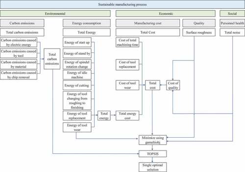
These five objective functions were solved simultaneously using the Gamultiobj algorithm (MATLAB). This algorithm finds Pareto front of multiple fitness functions using a Non-dominated Sorting Genetic Algorithm II (NSGA II). This algorithm is a fast and elitist multi-objective genetic algorithm. The algorithm uses Euclidean distance to select non-dominated solutions. Model’s structure, usefulness, optimization approach and metrics to select nondominated solutions are described in Deb et al. (2002). The best solution is determined using Technique for Order of Preference by Similarity to Ideal Solution (TOPSIS) which widely used to determine the best solution from a set of Pareto optimal solutions such as in Pawanr et al. (2019). TOPSIS is one of multi criteria decision making techniques which used to find a solution based on the smallest distance from the ideal positive solution and the farthest distance from the ideal negative solution (Hwang et al., 1993).

Our model development process is based on the relationship between the time required by the machining process and the power required to produce a unit product. This relationship is an essential consideration that will be used as a model development reference to ensure that the developed model is sufficiently close to a real system. Several previous models have considered the relationship between processing time and power per unit product (Shin et al., 2019; Tian et al., 2019; Yi et al., 2015; Zhang et al., 2017; Zhang et al., 2016). Figure 2 presents the relationship between the processing time and power per unit product derived in this study. This details the processing time and power, particularly the time and power required to change the tool between the roughing pass and finishing pass. Based on Figure 2 a mathematical model related to the objective functions per unit product and decision variables considered in this study was formulated. The notations used in this paper are listed in Appendix 1.

Figure 2. Relationship between processing time and the power per unit product.

2.1. Total machining time$\left(t_{total}\right)$

According to Figure 2, the total machining time is defined as one cycle time from startup to the finishing pass per unit product. The total machining time consists of a constant time and variable time. The constant time consists of the startup time and standby time. The variable time consists of the spindle rotation change time, idle time, machining time, time for tool changing from roughing to finishing, and total tool changing time.

2.1.1. Spindle rotation change time$\left(t_{src}\right)$

According to Figure 2, the spindle rotation change time consists of the acceleration and deceleration times for both the roughing and finishing passes. The spindle rotation change time per unit product is defined in Equation (1(1) $t_{src}=t_{sra\left(r\right)}+t_{srd\left(r\right)}+t_{sra\left(f\right)}+t_{srd\left(f\right)}$(1) ; Hu et al., 2019). Equations (2)(2) $t_{sra\left(r\right)}=\frac{2\pi \left(2\frac{v_{r,1}}{D_1}\right)}{60{\alpha }_a}$(2) to (5) define the acceleration and deceleration times for the roughing and finishing processes.

(1) $t_{src}=t_{sra\left(r\right)}+t_{srd\left(r\right)}+t_{sra\left(f\right)}+t_{srd\left(f\right)}$(1)

(2) $t_{sra\left(r\right)}=\frac{2\pi \left(2\frac{v_{r,1}}{D_1}\right)}{60{\alpha }_a}$(2)

(3) $t_{srd\left(r\right)}=\frac{-2\pi \left(2\frac{v_{r,n}}{D_1}\right)}{60{\alpha }_d}$(3)

(4) $t_{sra\left(f\right)}=\frac{2\pi \left(2\frac{v_f}{D_1}\right)}{60{\alpha }_a}$(4)

(5) $t_{srd\left(f\right)}=\frac{-2\pi \left(2\frac{v_f}{D_1}\right)}{60{\alpha }_d}$(5)

2.1.2. Idle time$\left(t_i\right)$

The idle time of the machining process can be divided into three stages based on the tool movement during the machining process, as shown in Figures 3 and 4. The first stage of the idle time consists of tool movement along the 1 r path. The second stage of idle time consists of tool movement after completing the first roughing pass (paths 3 r-4 r-5 r). The first stage of idle time occurs once for each machining process per unit product, whereas the second stage of idle time occurs for roughing passes two to $n$. Based on Figure 4, this paper proposes additional time for the finishing tool return (path 3 f) as the third stage of idle time. This idle time is defined in Equation (6)(6) $t_i=t_{i1}+t_{i2}+t_{i3}$(6) and the idle times of stages one, two, and three are defined in Equations (7)(7) $t_{i1}=\frac{\sqrt{{\left(Z_{Ot}-e_z\right)}^2+{\left(X_{Ot}-\frac{D_1}{2}-d_{r1}\right)}^2}}{v_0}$(7) , (8(8) $t_{i2}=\sum _{i=2}^{n-1}\left(\frac{\frac{e_x}{cos\alpha }+L-\frac{e_x}{tan\alpha }+e_z+e_x+d_{r,i}}{v_0}\right)$(8) ), and (9(9) $t_{i3}=\frac{\sqrt{{\left(Z_{Ot}+L\right)}^2+{\left(X_{Ot}-\left(\frac{D_1}{2}-{\sum }_{i=1}^n{d}_{r,i}-d_f\right)\right)}^2}}{v_0}$(9) ), respectively.

(6) $t_i=t_{i1}+t_{i2}+t_{i3}$(6)

(7) $t_{i1}=\frac{\sqrt{{\left(Z_{Ot}-e_z\right)}^2+{\left(X_{Ot}-\frac{D_1}{2}-d_{r1}\right)}^2}}{v_0}$(7)

(8) $t_{i2}=\sum _{i=2}^{n-1}\left(\frac{\frac{e_x}{cos\alpha }+L-\frac{e_x}{tan\alpha }+e_z+e_x+d_{r,i}}{v_0}\right)$(8)

(9) $t_{i3}=\frac{\sqrt{{\left(Z_{Ot}+L\right)}^2+{\left(X_{Ot}-\left(\frac{D_1}{2}-{\sum }_{i=1}^n{d}_{r,i}-d_f\right)\right)}^2}}{v_0}$(9)

Figure 3. Tool movement in roughing pass.

Figure 4. Tool movement in finishing pass.

2.1.3. Machining time$\left(t_m\right)$

The machining time is the specific time used by the tool to cut a workpiece. According to Figure 3, the machining time of the first roughing pass is defined by path 2 r. The machining time for the finishing pass is presented in Figure 4, as indicated by path 2 f. The machining time formulations used in this study are presented in ; (Arif et al., 2014; Bouzid, 2005; Chen & Tsai, 1996). The machining time equation for the multi-pass turning process consists of n roughing and finishing passes. Specifically, the machining time model for the roughing passes is defined in Equation (10) and the machining time for the finishing passes is defined in Equation (11). The machining time per unit product for n roughing and finishing passes is defined in Equation (12).

(9) $t_{mr}=\sum _{i=1}^n\frac{60\pi D_{i}L}{1000v_{r,i}{f}_{r,i}}$(9)

(9) $t_{mf}=\frac{60\pi D_{n+1}L}{1000v_f{f}_f}$(9)

(9) $t_m=t_{mr}+t_{mf}$(9)

2.1.4. Time for tool changing from the roughing to the finishing pass$\left(t_{trf}\right)$

According to Figure 3, there are three stages of tool changing from the roughing to the finishing pass. The first stage is the time required for tool movement after the nth roughing pass (B) to the tool home (Ot). The second stage is the fixed time required to change the roughing tool to the finishing tool with a value of $k_{trf}$. According to Figure 4, the third stage is the time required for tool movement from Ot to C. The time required for tool changing from the roughing to the finishing pass per unit product is defined in Equation (13)(13) $t_{trf}=t_{trf1}+k_{trf}+t_{trf2}$(13) . Equations (14)(14) $t_{trf1}=\frac{\sqrt{{\left(Z_{Ot}+L\right)}^2+{\left(X_{Ot}-\left(\frac{D_1}{2}-{\sum }_{i=1}^n{d}_{r,i}\right)\right)}^2}}{v_0}$(14) and (15(15) $t_{trf2}=\frac{\sqrt{{\left(Z_{Ot}-e_z\right)}^2+{\left(X_{Ot}-\left(\frac{D_1}{2}-{\sum }_{i=1}^n{d}_{r,i}\right)\right)}^2}}{v_0}$(15) ) present the formulas for the first and third tool change times, respectively.

(13) $t_{trf}=t_{trf1}+k_{trf}+t_{trf2}$(13)

(14) $t_{trf1}=\frac{\sqrt{{\left(Z_{Ot}+L\right)}^2+{\left(X_{Ot}-\left(\frac{D_1}{2}-{\sum }_{i=1}^n{d}_{r,i}\right)\right)}^2}}{v_0}$(14)

(15) $t_{trf2}=\frac{\sqrt{{\left(Z_{Ot}-e_z\right)}^2+{\left(X_{Ot}-\left(\frac{D_1}{2}-{\sum }_{i=1}^n{d}_{r,i}\right)\right)}^2}}{v_0}$(15)

2.1.5. Time for tool replacement$\left(t_{tr}\right)$

During the machining process for p products, the tool must be sharpened or replaced. The tool replacement time per unit product is related to the tool life. The time of tool replacement per unit product is determined by multiplying the time for tool replacement per edge by the total number of edges per unit product. The time for tool replacement for the multi-pass turning process is defined in Equation (16)(16) $t_{tr}=t_e\left(\frac{t_m}{T}\right)$(16) . Tool life (Equation 17(17) $T=\theta T_r+\left(1-\theta \right)T_f$(17) ) has two components, namely the tool life for roughing and that for finishing, as defined in Equations (18)(18) $T_r=\sum _{i=1}^n\frac{60Co}{v_{r,i}^p{f}_{r,i}^q{d}_{r,i}^r}$(18) and (19(19) $T_f=\frac{60Co}{v_f^p{f}_f^q{d}_f^r}$(19) ), respectively.

(16) $t_{tr}=t_e\left(\frac{t_m}{T}\right)$(16)

(17) $T=\theta T_r+\left(1-\theta \right)T_f$(17)

(18) $T_r=\sum _{i=1}^n\frac{60Co}{v_{r,i}^p{f}_{r,i}^q{d}_{r,i}^r}$(18)

(19) $T_f=\frac{60Co}{v_f^p{f}_f^q{d}_f^r}$(19)

Based on these time elements, the total time required for the machining process per unit product is defined in Equation (20)(20) $t_{total}=t_{su}+t_{sb}+t_{tscr}+t_i+t_m+t_{trf}+t_{tr}$(20) .

(20) $t_{total}=t_{su}+t_{sb}+t_{tscr}+t_i+t_m+t_{trf}+t_{tr}$(20)

2.2. Total energy consumptions$\left(E_{total}\right)$

Our model formulation for total energy consumption is based on Figure 3. Based on the considered decision variables, energy consumption is divided into two categories. Energy consumption is not influenced by the decision variables for startup and standby energy consumption, but it is influenced by the other decision variables. The second category includes spindle rotation change, idle machine, machining, tool changing from the roughing to the finishing pass, tool replacement, and tool wear energy consumption. The startup energy consumption $\left(E_{su}\right)$ is the energy required during the startup time. According to Figure 3, by assuming that the power increase is linear, the energy consumption is determined to be the product of half of the startup time and startup power. The start-up energy consumption is defined in Equation (21)(21) $E_{su}=\frac{1}{2}{P}_{su}.t_{su}$(21) . The standby energy consumption $\left(E_{sb}\right)$ is the energy required during standby time, as shown in Equation (22)(22) $E_{sb}=P_{sb}{t}_{sb}$(22) .

(21) $E_{su}=\frac{1}{2}{P}_{su}.t_{su}$(21)

(22) $E_{sb}=P_{sb}{t}_{sb}$(22)

The spindle rotation changes energy consumption $\left(E_{src}\right)$ is the energy required for acceleration and deceleration. It consists of four elements: the acceleration energy consumption of the roughing pass, deceleration energy consumption of the roughing pass, acceleration energy consumption of the finishing pass, and deceleration energy consumption of the finishing pass. The energy consumption for spindle rotation change is defined in Equation (23)(23) $E_{src}=E_{sra\left(r\right)}+E_{srd\left(r\right)}+E_{sra\left(f\right)}+E_{srd\left(f\right)}$(23) . The elements of this energy consumption are defined in Equations (24)(24) $E_{sra\left(r\right)}=\frac{1}{2}{P}_{sra\left(r\right)}{t}_{sra\left(r\right)}$(24) to (27). The idle machine energy consumption $\left(E_i\right)$ can be determined by multiplying the idle power by the idle time, as shown in Equation (28)(28) $E_i=P_i{t}_i$(28) .

(23) $E_{src}=E_{sra\left(r\right)}+E_{srd\left(r\right)}+E_{sra\left(f\right)}+E_{srd\left(f\right)}$(23)

(24) $E_{sra\left(r\right)}=\frac{1}{2}{P}_{sra\left(r\right)}{t}_{sra\left(r\right)}$(24)

(25) $E_{srd\left(r\right)}=\frac{1}{2}{P}_m{t}_{srd\left(r\right)}$(25)

(26) $E_{sra\left(f\right)}=\frac{1}{2}{P}_{sra\left(f\right)}{t}_{sra\left(f\right)}$(26)

(27) $E_{srd\left(f\right)}=\frac{1}{2}{P}_m{t}_{srd\left(f\right)}$(27)

(28) $E_i=P_i{t}_i$(28)

The machining energy consumption $\left(E_m\right)$ is the energy required during workpiece cutting. The machining energy consumption $\left(E_m\right)$ is determined by multiplying the machining power (P_m) by the machining time (t_m). As shown in Figure 2, P_tool is the power required to remove material. If the material removal rate (MRR) is assumed to be constant, then P_tool is also constant (Du et al., 2020; Pawanr et al., 2021). P_tool has a functional relationship with MRR in terms of the specific energy used for cutting operations (k; Du et al., 2020; Nur et al., 2015). As shown in Figure 2, P_tool is one component of P_m. The machining energy consumption consists of the energy consumption of the roughing and finishing passes. Equation (29)(29) $E_m=E_{mr}+E_{mf}$(29) defines the machining energy consumption, and Equations (30)(30) $E_{mr}=\sum _{i=1}^n{P}_m{t}_{mr,i}$(30) and (31(31) $E_{mf}=P_m{t}_{mf}$(31) ) represent the machining energy consumption of the roughing and finishing passes, respectively.

(29) $E_m=E_{mr}+E_{mf}$(29)

(30) $E_{mr}=\sum _{i=1}^n{P}_m{t}_{mr,i}$(30)

(31) $E_{mf}=P_m{t}_{mf}$(31)

The energy consumption for tool changing from the roughing to the finishing pass $\left(E_{trf}\right)$ is determined by multiplying the power and time required for changing the roughing tool to the finishing tool, as shown in Equation (32)(32) $E_{trf}=P_{trf}{t}_{trf}$(32) . Tool replacement energy consumption occurs when the tool module is active and the power is in the standby condition (Arif et al., 2014). The tool replacement energy consumption $\left(E_{tr}\right)$ is then calculated as the product of the standby power, total number of cutting edges per unit product, and tool replacement time per edge, as shown in Equation (33(33) $E_{tr}=P_{sb}{t}_e\left(\frac{t_m}{T}\right)$(33) ; Lu et al., 2016). The tool wear energy consumption $\left(E_{tw}\right)$ is defined as the tool energy footprint per edge per piece, which represents the energy contained in the tool, energy consumed for tool manufacturing, and energy consumed for tool coating (Arif et al., 2014). Equation (34)(34) $E_{tw}=P_{tw}\frac{t_m}{T}$(34) defines the tool-wear energy consumption (Lu et al., 2016).

(32) $E_{trf}=P_{trf}{t}_{trf}$(32)

(33) $E_{tr}=P_{sb}{t}_e\left(\frac{t_m}{T}\right)$(33)

(34) $E_{tw}=P_{tw}\frac{t_m}{T}$(34)

Based on these energy consumption elements, the total energy consumption for the machining process per unit product is defined in Equation (35)(35) $E_{total}=E_{su}+E_{sb}+E_i+E_{trf}+E_{tscr}+E_m+E_{tr}+E_{tw}$(35) .

(35) $E_{total}=E_{su}+E_{sb}+E_i+E_{trf}+E_{tscr}+E_m+E_{tr}+E_{tw}$(35)

2.3. Surface roughness$\left(R_a\right)$

The product quality following the turning process must meet standard specifications. One of the product qualities considered in the turning process is surface roughness, which is an important quality characteristic (Phadke, 1989). There are two methods for considering surface roughness in the turning process model: the objective function and the constraint function (Jiang et al., 2019; Lu et al., 2016; Schultheiss et al., 2017). In a previous study, the surface roughness function was expressed as a regression function that was obtained experimentally (Jiang et al., 2019). However, we adopt the function in Equation (36)(36) $R_a=0.77\left(r_f-\frac{{r_f}^2}{f_f}si{n}^{-1}\left(\frac{f_f}{2r_f}\right)-\frac{r_f}{2}\sqrt{1-\frac{f_f^2}{4{r_f}^2}}\right)$(36) to represent surface roughness, which was taken from Stahl et al. (Ståhl et al., 2011).

(36) $R_a=0.77\left(r_f-\frac{{r_f}^2}{f_f}si{n}^{-1}\left(\frac{f_f}{2r_f}\right)-\frac{r_f}{2}\sqrt{1-\frac{f_f^2}{4{r_f}^2}}\right)$(36)

2.4. Total noise$\left(B_{total}\right)$

The total noise generated by the turning process affects worker health. In a previous study, the total noise was not included in the turning process model. The total noise objective function used in this study adopts a quadratic function formula taken from Cirtu et al. (1976) and Olaru et al. (2017). In these two studies, a total noise objective function for the multi-pass turning process was not formulated. In this study, total noise has two components, namely noise originating from the roughing and finishing passes. The formulas for the total noise objective function and the components are presented in Equations (37)(37) $B_{total}=\sum _{i=1}^n{B}_{r,i}+B_f$(37) to (39).

(37) $B_{total}=\sum _{i=1}^n{B}_{r,i}+B_f$(37)

(38) $B_{r,i}=a_{ns}{P}_m+b_{ns}\left(\frac{v_{r,i}}{f_{r,i}}\right)+c_{ns}\left(P_m\times \left(\frac{v_{r,i}}{f_{r,i}}\right)\right)+n.B_m,i=\mathrm{1..}n$(38)

(39) $B_f=a_{ns}{P}_m+b_{ns}\frac{v_f}{f_f}+c_{ns}\left(P_m\times \frac{v_f}{f_f}\right)+B_m$(39)

2.5. Total cost$\left(C_{total}\right)$

The total cost consists of machining, tool replacement, tool wear, and idle machine costs (Liu et al., 2016). Other studies have considered total energy costs (Bagaber & Yusoff, 2019; Pangestu et al., 2021; Tian et al., 2019). However, previous studies did not include the cost of quality loss. We adopted Taguchi’s quality loss function to calculate the cost of quality loss caused by surface roughness and total noise. The machining cost $\left(C_m\right)$ is formulated based on direct and overhead labor costs, which are multiplied by the total machining time. The machining cost formula is defined in Equation (40)(40) $C_m=k_o{t}_{total}$(40) . The idle machine cost $\left(C_i\right)$ is the product of the direct and overhead labor costs multiplied by the idle machine time. The idle machine cost formula is defined in Equation (41)(41) $C_i=k_o{t}_i$(41) . The tool replacement cost $\left(C_{tr}\right)$ is the product of the direct and overhead labor costs and the tool replacement time. The tool replacement cost is defined in Equation (42)(42) $C_{tr}=k_0\left(t_e\left(\frac{t_m}{T}\right)\right)$(42) . The tool wear cost $\left(C_{tw}\right)$ is the product of the tool cost and the number of cutting edges per unit product, as defined in Equation (43)(43) $C_{tw}=k_t\left(\frac{t_m}{T}\right)$(43) . The total energy cost $\left(C_e\right)$ is dependent on the cost of the electricity used during the multi-pass turning process per unit product. The total energy cost is the product of the electricity cost coefficient and total energy, as shown in Equation (44)(44) $C_e=x_e\times E_{total}$(44) .

(40) $C_m=k_o{t}_{total}$(40)

(41) $C_i=k_o{t}_i$(41)

(42) $C_{tr}=k_0\left(t_e\left(\frac{t_m}{T}\right)\right)$(42)

(43) $C_{tw}=k_t\left(\frac{t_m}{T}\right)$(43)

(44) $C_e=x_e\times E_{total}$(44)

In this research, the quality cost $\left(C_q\right)$ is represented by loss to society in term of personal health and economic loss in term of surface roughness. Those losses are converted into monetary values using Taguchi loss function in which both the total noise and surface roughness are smaller are better characteristics. The quality cost of surface roughness is the product of the quality cost constant related to surface roughness and the square of the surface roughness, as shown in Equation (45)(45) $C_{q1}=k_{q1}\times R_a^2$(45) . The quality cost of the total noise is the product of the quality cost constant related to the total noise and the square of the total noise, as shown in Equation (46)(46) $C_{q2}=k_{q2}\times B_{total}^2$(46) . The quality cost is the sum of the quality cost of the surface roughness and the quality cost of the total noise, as shown in Equation (47)(47) $C_q=C_{q1}+C_{q2}$(47) .

(45) $C_{q1}=k_{q1}\times R_a^2$(45)

(46) $C_{q2}=k_{q2}\times B_{total}^2$(46)

(47) $C_q=C_{q1}+C_{q2}$(47)

Based on these cost elements, the total cost for the multi-pass turning process per unit product is formulated in Equation (48)(48) $C_{total}=C_m+C_i+C_{tr}+C_{tw}+C_e+C_q$(48) .

(48) $C_{total}=C_m+C_i+C_{tr}+C_{tw}+C_e+C_q$(48)

2.6. Total carbon emissions$\left(C{E}_{total}\right)$

The total carbon emission model is based on a previous study that did not consider the multi-pass turning process (Li et al., 2013; Liu et al., 2016). The total carbon emission consists of the carbon emissions related to electrical energy consumption, cutting tools, raw material consumption, and chip disposal. The carbon emission of electrical energy consumption $\left(C{E}_{el}\right)$ is expressed in Equation (49)(49) $C{E}_{el}=CE{F}_{el}\times E_{total}$(49) as the product of a constant related to the carbon emissions caused by electrical energy consumption and the total energy. The carbon emission of the cutting tool $\left(C{E}_{tool}\right)$ stems from the production of the cutting tool, as indicated in Equation (50)(50) $C{E}_{tool}=\frac{t_m}{T}\times \left(CE{F}_{tool}+W_{tool}\right)$(50) . The carbon emission of the raw materials $\left(C{E}_{mr}\right)$ is expressed as a function of the mass of the material removed during the roughing and finishing passes, as shown in Equations (51)(51) $C{E}_{mr}=CE{F}_{mr}\times M_{chip}$(51) to (54). Equation (55)(55) $C{E}_{chip}=CE{F}_{chip}\times M_{chip}$(55) represents the carbon emission from chip disposal. Based on these carbon emissions elements, the total carbon emissions formula for the multi-pass turning process per unit product is defined in Equation (56)(56) $C{E}_{total}=C{E}_{el}+C{E}_{tool}+C{E}_{mr}+C{E}_{chip}$(56) .

(49) $C{E}_{el}=CE{F}_{el}\times E_{total}$(49)

(50) $C{E}_{tool}=\frac{t_m}{T}\times \left(CE{F}_{tool}+W_{tool}\right)$(50)

(51) $C{E}_{mr}=CE{F}_{mr}\times M_{chip}$(51)

(52) $M_{chip}=M_{chip\left(r,i\right)}+M_{chip\left(f\right)}$(52)

(53) $M_{chip\left(r,i\right)}={10}^{-6}.\pi DL\left(d_t-d_f\right)\rho$(53)

(54) $M_{chip\left(f\right)}={10}^{-6}.\pi DL\rho$(54)

(55) $C{E}_{chip}=CE{F}_{chip}\times M_{chip}$(55)

(56) $C{E}_{total}=C{E}_{el}+C{E}_{tool}+C{E}_{mr}+C{E}_{chip}$(56)

2.7. Objective and constraint functions

Based on the model development for machining parameters discussed in Subsections 2.2 to 2.6, the objective functions for the proposed model are the total energy (f₁; Equation (35)(35) $E_{total}=E_{su}+E_{sb}+E_i+E_{trf}+E_{tscr}+E_m+E_{tr}+E_{tw}$(35) ), surface roughness (f₂; Equation (36)(36) $R_a=0.77\left(r_f-\frac{{r_f}^2}{f_f}si{n}^{-1}\left(\frac{f_f}{2r_f}\right)-\frac{r_f}{2}\sqrt{1-\frac{f_f^2}{4{r_f}^2}}\right)$(36) ), total noise (f₃; Equation (37)(37) $B_{total}=\sum _{i=1}^n{B}_{r,i}+B_f$(37) ), total costs (f₄; Equation (48)(48) $C_{total}=C_m+C_i+C_{tr}+C_{tw}+C_e+C_q$(48) ), and total carbon emission (f₅; Equation (56)). The optimal machining parameters must be appropriate for the constraint functions. The constraint functions used in this study are the depth of the cut, cutting speed, feed rate, tool life, cutting force, power, stable cutting region, and chip-tool interface temperature. The constraints related to the solution space are the cutting speed, feed rate, and depth of cut in the form of lower and upper bounds. The tool life constraint is required to achieve optimal manufacturing cost and product quality. The cutting force constraint is required to avoid the uncontrollable deflection of tools and workpieces. The cutting power constraint is required to achieve optimal energy consumption. The stable cutting region constraint is required to prevent vibration and adhesion. The chip-tool interface temperature must be limited to improve tool life. The higher the temperature, the shorter the tool life. The depth of cut and feed rate in the roughing pass are typically greater than those in the finishing pass. Each of these constraints is applied in both the roughing and finishing passes of the turning process. These parameter relationship constraints are suitable for our model. The constraint functions adopted in this study refer to those in previous studies (Arif et al., 2014; Lu et al., 2016), as shown in Equations (57)(57) $v_{rL}\le v_{r,i}\le v_{rU}$(57) to (77).

2.8. The roughing pass constraints

The cutting speed

(57) $v_{rL}\le v_{r,i}\le v_{rU}$(57)

The feed rate

(58) $f_{rL}\le f_{r,i}\le f_{rU}$(58)

The depth of cut

(59) $d_{rL}\le d_{r,i}\le d_{rU}$(59)

The tool life

(60) $T_{rL}\le T_r\le T_{rU}$(60)

The cutting force

(61) $k_1{f}_{r,i}^{\mu }{d}_{r,i}^{\vartheta }\le F_U$(61)

The cutting power

(62) $\frac{k_1{v}_{r,i}{f}_{r,i}^{\mu }{d}_{r,i}^{\vartheta }}{6120\eta }\le P_U$(62)

The stable cutting region

(63) $v_{r,i}^{\lambda }{f}_{r,i}{d}_{r,i}^v\ge S_c$(63)

The chip-tool interface temperature

(64) $k_2{v}_{r,i}^{\tau }{f}_{r,i}^{\phi }{d}_{r,i}^{\delta }\le Q_U$(64)

2.9. The finishing pass constraints

The cutting speed

(65) $v_{fL}\le v_f\le v_{fU}$(65)

The feed rate

(66) $f_{fL}\le f_f\le f_{fU}$(66)

The depth of cut

(67) $d_{fL}\le d_f\le d_{fU}$(67)

The tool life

(68) $T_{fL}\le T_f\le T_{fU}$(68)

The cutting force

(69) $k_1{f}_f^{\mu }{d}_f^{\vartheta }\le F_U$(69)

The cutting power

(70) $\frac{k_1{v}_f{f}_f^{\mu }{d}_f^{\vartheta }}{6120\eta }\le P_U$(70)

The stable cutting region

(71) $v_f^{\lambda }{f}_f{d}_f^v\ge S_c$(71)

The chip-tool interface temperature

(72) $k_2{v}_f^{\tau }{f}_f^{\phi }{d}_f^{\delta }\le Q_U$(72)

2.10. The parameter relationships

The cutting speed

(73) $v_f\ge k_3{v}_{r,i}$(73)

The feed rate

(74) $f_{r,i}\ge k_4{f}_f$(74)

The depth of cut

(75) $d_{r,i}\ge k_5{d}_f$(75)

The total deep of cut

(76) $d_t=d_f+\sum _{i=1}^n{d}_{r,i}$(76)

The number roughing passes

(77) $n_L\le n\le n_U,\hspace{0.17em}n=\mathrm{i}\mathrm{n}\mathrm{t}\mathrm{e}\mathrm{g}\mathrm{e}\mathrm{r}$(77)

3. Numerical examples and analysis

The parameter values used for the numerical example in this study were taken from previous studies (Cirtu et al., 1976; Hu et al., 2019; Lu et al., 2016; Olaru et al., 2017; Tian et al., 2019). The workpiece used in the numerical example is made of carbon steel C45. The diameter $\left(D\right)$ of the workpiece is 80 mm and the length $\left(L\right)$ is 200 mm. The total cutting depth $\left(d_t\right)$ of the workpiece is 10 mm. The cutting tool specifications are listed in Table 2 and the constants related to the tool are listed in Table 3. Tables 4 - 8 list the parameters related to the machining time, total energy, surface roughness, total noise, total cost, total carbon emission, and constraint functions. All of these parameters were substituted into the equations representing the objective functions and constraints of the model. We assumed in this numerical example that the operator wears the protective personal equipment to reduce the effects of noise and prevent the occurrence of accidents. Additional environmental conditions like temperature, humidity, and vibration will be considered in a future study.

Table 2. Tool specifications (modified from Lu et al., 2016)

Parameter	Roughing	Finishing
Hardness	69–81 HRC	69–81 HRC
Tool lead angle	45°	45°
Rake angle	20°	20°
Inclination angle	5°	5°
Radius	1.2 mm	0.8 mm

Table 3. Constants related to the tool (modified from Lu et al., 2016)

Parameter	Roughing	Finishing
$C_0$	$6\times {10}^{11}$	$6\times {10}^{11}$
$p$	5	5
$q$	1.75	1.75
$r$	0.75	0.75

Table 4. Parameter values related to the machining process (modified from Lu et al., 2016)

Notation	Value	Notation	Value
$\alpha$	45°	$v_0$	800 m/min
${\alpha }_a$	39.78	$X_{Ot}$	100 mm
${\alpha }_d$	−38.79	$Z_{Ot}$	100 mm
$\theta$	0.5	$t_e$	0.75 min/edge
$e_x$	1 mm	$t_{su}$	0.06 second
$e_z$	1 mm	$t_{sb}$	4 second

Table 5. Parameter values related to energy consumption

Notation	${\mathit{P}}_{\mathit{s}\mathit{u}}$	${\mathit{P}}_{\mathit{s}\mathit{b}}$	${\mathit{P}}_{\mathit{s}\mathit{r}\mathit{a}}$	${\mathit{P}}_{\mathit{m}}$	${\mathit{P}}_{\mathit{i}}$	${\mathit{P}}_{\mathit{t}\mathit{r}\mathit{f}}$	${\mathit{P}}_{\mathit{t}\mathit{w}}$
Value	1600 W	300 W	1500 W	1300 W	1100 W	600 W	1600 W

Table 6. Parameter values related to noise (modified from Cirtu et al., 1976; Olaru et al., 2017)

Notation	${\mathit{a}}_{\mathit{n}\mathit{s}}$	${\mathit{b}}_{\mathit{n}\mathit{s}}$	${\mathit{c}}_{\mathit{n}\mathit{s}}$	${\mathit{B}}_{\mathit{m}}$
Value	0.17	$-1.4\times {10}^{-5}$	$0.6\times {10}^{-5}$	78.7

Table 7. Parameter values related to total cost (Tian et al., 2019)

Notation	${\mathit{k}}_{\mathit{t}}$	${\mathit{k}}_{\mathit{o}}$	${\mathit{k}}_{\mathit{q}\mathbf{1}}$	${\mathit{k}}_{\mathit{q}\mathbf{2}}$	${\mathit{x}}_{\mathit{e}}$
Value	0.15 $/edge	0.002 $/sec	0.001 $	1 $\times {10}^{-5}$ $	5.8 $\times {10}^{-4}$ $/Joule

Table 8. Parameter values related to carbon emission (Tian et al., 2019)

Notation	$\mathit{C}E{F}_{el}$	$\mathit{C}E{F}_{tool}$	${\mathit{W}}_{\mathit{t}\mathit{o}\mathit{o}\mathit{l}}$	$\mathit{C}E{F}_{mr}$	$\mathit{C}E{F}_{chip}$	$\mathit{\rho }$
Value	0.6747 kgCO2/kWh	29.6 kgCO2/kg	9.5 gr	16.13 kgCO2/kg	0,361 kgCO2/kg	7.1 g/cm^3

There were two stages to find the single optimal solution to minimize $\left(f_1,f_2,f_3,f_4,f_5\right)$ subject to Equations (57)(57) $v_{rL}\le v_{r,i}\le v_{rU}$(57) to (77). The first stage was to find the Pareto frontiers set for all five objective functions. In the second stage is to find the Pareto point to get the single optimal solution. Finding the Pareto point to get the single optimal solution is difficult (Costa & Lourenço, 2017). Some of the methods applied are hypervolume under the Pareto front (Lu and Anderson-Cook, 2013). In this study, the single optimal solution will be found using TOPSIS method. The TOPSIS method for selecting a single optimal solution from a set of Pareto points was also carried out by Chen et al. (2022) and Faghiri et al. (2022).

The first stage that to find the Pareto frontiers set, the proposed model was solved using the Gamultiobj function in MATLAB 2020a (MATLAB, 2020). The gamultiobj algorithm is also used for multi objective optimization including Sellami et al. (2020) and Kallio and Siroux (2021). Four setting parameter values were used to run the Gamultiobj algorithm to find the Pareto frontiers. The four parameter settings are run for number of roughing passes (n) equal to 3,4 and 5. The first setting parameter value for the number of roughing passes (n) = 3 because of the total cutting depth of the workpiece is 10 mm. Meanwhile, the upper bound of the depth of cut in roughing passes and finishing pass is 3 mm. The finishing pass is determined once, so it takes a minimum of 3 roughing passes before the finishing pass. Table 9 shows parameter values related to constraint functions and Table 10 shows setting parameter values in Gamultiobj algorithm.

Table 9. Parameter values related to constraint functions (Lu et al., 2016)

Notation	Value	Notation	Value	Notation	Value
$\mu$	0.75	$d_{fL}$	1 mm	$k_5$	1
$\vartheta$	0.95	$d_{fU}$	3 mm	$n_L$	3
$\eta$	0.85	$f_{rL}$	0.1 mm/rev	$n_U$	9
$\lambda$	2	$f_{rU}$	0.9 mm/rev	$P_U$	5000 W
$v$	−1	$F_U$	4903.33 kgf	$Q_U$	1000°C
$\tau$	0.4	$f_{fL}$	0.1 mm/rev	$S_C$	140
φ	0.2	$f_{fU}$	0.9 mm/rev	$T_L$	1500 sec
$\delta$	0.105	$k_1$	108	$T_U$	2700 sec
$d_t$	10 mm	$k_2$	132	$v_{fL}$	50 m/min
$d_{rL}$	1 mm	$k_3$	1	$v_{fU}$	500 m/min
$d_{rU}$	3 mm	$k_4$	2.5

Table 10. Setting parameter values in gamultiobj algorithm

Parameters	Values
	Setting #1	Setting #2	Setting #3	Setting #4
Population size	200	250	300	300
Initial population range	[−10,10]	[−100,100]	[−1000,1000]	[−10,10]
Probability of crossover	0.80	0.60	0.70	0.80
Probability of migration	0.20	0.15	0.25	0.20
Pareto front population fraction	0.35	0.30	0.25	0.35
Maximum number of generations	1200	1300	1400	1200

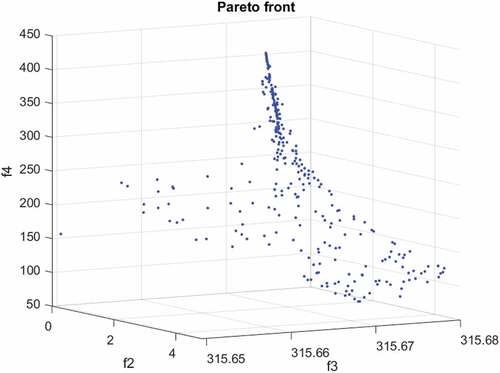
In this paper, the calculation and the results of the Pareto frontier are only for the first setting parameter value and for the number of roughing passes (n) = 3. There were 200 points of Pareto front corresponding to non-dominated solutions for the first setting and n = 3. Ideally, with five objective functions, the Pareto front graph should be shown in five dimensions (5D). Since it is impossible to draw the Pareto graph in 5D, we show the Pareto graph in two dimensions (2D) and three dimensions (3D) for all possible combinations. The number of combinations for both 2D and 3D Pareto fronts graph are 10. Four Pareto front graph (Figures 5 to 8) are shown consecutively in the next section, while the rest of combination are provided in Appendix 2. Figure 5 presents 2D of the Pareto front graph and the tradeoff between the total energy (f₁) and total noise (f₃). Figure 6 presents 2D of the Pareto front graph and the tradeoff between the surface roughness (f₂) and total cost (f₄). Figure 7 presents 3D of the Pareto front and the tradeoff between the total energy (f₁), surface roughness (f₂), and total noise (f₃). Figure 8 presents 3D of the Pareto front graph and the tradeoff between surface roughness (f₂), total noise (f₃), and total cost (f₄).

Figure 5. Pareto front for ${\mathit{f}}_{\mathbf{1}}\mathrm{a}\mathrm{n}\mathrm{d}{f}_3$.

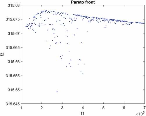
Figure 6. Pareto front for ${\mathit{f}}_{\mathbf{2}}\mathrm{a}\mathrm{n}\mathrm{d}{f}_4$.

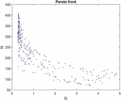
Figure 7. Pareto front for ${\mathit{f}}_{\mathbf{1}},f_2,\mathrm{a}\mathrm{n}\mathrm{d}{f}_3$.

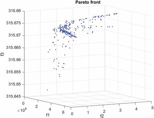
Figure 8. Pareto front for ${\mathit{f}}_{\mathbf{2}},f_3,\mathrm{a}\mathrm{n}\mathrm{d}{f}_4$.

After identifying the non-dominated solutions (Pareto front) using the Gamultiobj algorithm, the next stage is to determine a single best solution using the TOPSIS method. There were 200 points corresponding to non-dominated solutions (Pareto front), among which the best solution was identified using TOPSIS. There are seven steps in the TOPSIS method to determine a single optimal solution. Tables 11-18 show the process of finding a single optimal solution using TOPSIS for the first setting parameter value and the number of roughing passes (n) equals 3.

1. Create an evaluation matrix, $\left(a_{ij}\right)A\times F$, consisting of A alternatives and F criteria. In this case, A are 200 points corresponding to non-dominated solutions and F are objective functions.

2. Normalize evaluation matrix using this formula ${\alpha }_{ij}=\frac{a_{ij}}{\sqrt{{\sum }_{i=1}^{200}{\left(a_{ij}\right)}^2}}$

• (3) Calculate the weighted normalized decision matrix, ${\chi }_{ij}={\alpha }_{ij}\ast {\omega }_j$.

Table 11. Matrix A alternatives and F criteria

	f1	f2	f3	f4	f5
A1	626,612.881	0.277	315.674	364.508	425,912.242
A2	321,669.264	1.229	315.677	187.171	220,154.330
…	…	…	…	…	…
A30	665,750.575	0.299	315.674	387.268	452,316.618
A31	693,731.137	0.295	315.674	403.540	471,195.082
…	…	…	…	…	…
A199	599,716.924	0.285	315.674	348.867	407,765.540
A200	616,377.864	0.384	315.674	358.556	419,005.025

Table 12. Normalize matrix A alternatives and F criteria

	f1	f2	f3	f4	f5
A1	0.1047	0.0106	0.0707	0.1047	0.1045
A2	0.0538	0.0472	0.0707	0.0538	0.0540
…	.	…	…	…	…
A30	0.1113	0.0115	0.0707	0.1113	0.1110
A31	0.1160	0.0113	0.0707	0.1159	0.1156
…	.	…	…	…	…
A199	0.1002	0.0109	0.0707	0.1002	0.1000
A200	0.1030	0.0148	0.0707	0.1030	0.1028

Table 13. Weighted normalize matrix $\left({\chi }_{ij}\right)$

	f1	f2	f3	f4	f5
A1	0.0209	0.0011	0.0071	0.0209	0.0418
A2	0.0108	0.0047	0.0071	0.0108	0.0216
…	.	…	…	…	…
A30	0.0223	0.0011	0.0071	0.0223	0.0444
A31	0.0232	0.0011	0.0071	0.0232	0.0462
…	.	…	…	…	…
A199	0.0200	0.0011	0.0071	0.0200	0.0400
A200	0.0206	0.0015	0.0071	0.0206	0.0411

Table 14. Maximum and minimum alternative

	f1	f2	f3	f4	f5
${\mathrm{A}}_{\mathrm{j}}^{+}$	0.0232	0.0188	0.0071	0.0232	0.0462
${\mathrm{A}}_{\mathrm{j}}^{-}$	0.0038	0.0011	0.0071	0.0038	0.0079

Table 15. Euclidean distance between the target

	d^+	d^−		d^+	d^−		d^+	d^−
A1	0.0186	0.0417	A30	0.0178	0.0449	A199	0.0193	0.0395
A2	0.0334	0.0173	A31	0.0177	0.0471	A200	0.0185	0.0408

Table 16. TOPSIS scores

	Si		Si		Si
A1	0.6916	A30	0.7156	A199	0.6716
A2	0.3408	A31	0.7270	A200	0.6888

Table 17. Minimum objective function values for setting #1 and n = 3

	Minimum value of objective functions
	f1	f2	f3	f3	f5
A31	693,731.137	0.295	315.674	403.540	471,195.082

Table 18. Decision variables values for setting #1 and n = 3

	Decision variables
	vr1	vr2	vr3	vf	fr1	fr2	fr3	ff	dr1	dr2	dr3	df
A31	50.012	50.200	50.460	50.765	0.284	0.270	0.272	0.102	2.954	2.954	2.954	1.136

Where ${\omega }_j=\frac{w_j}{{\sum }_{j=1}^5{w}_j}$, $\sum _{j=1}^5{\omega }_j=1$, where weight for f₁ = 0.20, f₂ = 0.10, f₃ = 0.10, f₄ = 0.20 and f₅ = 0.40

• (4) Determine the maximum $\left(A_j^{+}\right)$ and the minimum $\left(A_j^{-}\right)$ alternative for each criterion:

$A_j^{+}=ma{x}_{i=1}^{200}{\chi }_{ij},A_j^{-}=mi{n}_{i=1}^{200}{\chi }_{ij}$

• (5) Calculate the Euclidean distance between the target alternative and the maximum $\left(d_i^{+}\right)$ and minimum $\left(d_i^{-}\right)$ alternative: $d_i^{+}=\sqrt{\sum _{j=1}^5{\left({\chi }_{ij}-{\chi }_j^{+}\right)}^2}$, $d_i^{-}=\sqrt{\sum _{j=1}^5{\left({\chi }_{ij}-{\chi }_j^{-}\right)}^2}$

• (6) For each alternative calculate the similarity to the minimum alternative using $S_i=\frac{d_i^{-}}{d_i^{-}+d_i^{+}}$. The results are TOPSIS scores.

• (7) Find the maximum TOPSIS score. The maximum TOPSIS score is 0.7270 in A31.The maximum score TOPSIS score is correspondence with the optimal single solution.

Another combination of setting parameter values and the number of roughing passes (n) run in the similar method and stage. The first stage is to find the Pareto front and the second stage is to find a single optimal solution with TOPSIS. Table 19 shows the minimum objective function values of twelve runs for all combinations of four setting parameter values and number of roughing passes (n) equal to 3,4, and 5. Decision variables and minimum objective function values for all combinations are shown in Appendix 3.

Table 19. Minimum objective function values

n	Setting #	Minimum value of objective function (unit)
		f1 (Joule)	f2 (μm)	f3 (dBA)	f4 ($)	f5(KgCO2)
3	1	693,731.137	0.295	315.674	403.540	471,195.082
	2	730,090.821	0.280	315.673	424.684	495,719.297
	3	703,671.030	0.279	315.673	409.319	477,894.118
	4	697,487.052	0.304	315.674	405.723	473,722.563
4	1	495,965.751	0.285	393.938	288.587	337,748.265
	2	619,725.739	0.315	393.936	360.558	421,248.699
	3	674,179.007	0.312	393.937	392.225	457,981.263
	4	755,235.909	0.289	393.936	439.362	512,670.216
5	1	511,346.501	0.308	472.606	297.607	348,116.406
	2	526,719.268	0.283	472.605	306.547	358,488.573
	3	547,142.796	0.288	472.605	318.424	372,263.340
	4	530,452.464	0.290	472.605	308.717	361,002.225

It is more difficult to determine the effect of setting parameters and number of roughing passes (n) on the optimal solution. Based on Table 19 and Figures 9-13, if analyzed based on parameter settings, the first parameter setting gives optimal results for the objective functions f₁,f₄, and f₅. Suppose analyzed based on the number of roughing passes, the number of roughing passes (n) equals 4 providing optimal results for the objective functions f₁,f₃,f₄, and f₅. Generally, the minimum values of the five objective functions are associated with the first parameter setting, and the number of roughing passes (n) equals 4. The interesting results are emerged in the objective function, mainly the f₃ (noise). From the total noise with roughing pass (n) = 4, the average noise for the roughing and finishing passes is 78.788 dBA. This noise value is below the maximum noise limit of 85 dBA based on the Indonesia National Standard (SNI 16-7063-2004), for an operator works without using ear protection.

Figure 9. Effect of setting and n on f_1.

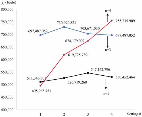
Figure 10. Effect of setting and n on f_2.

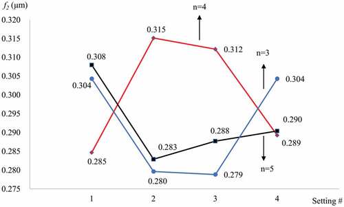
Figure 11. Effect of setting and n on average f_3.

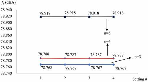
Figure 12. Effect of setting and n on f_4.

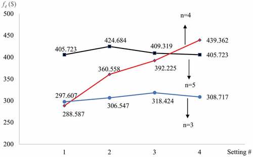
Figure 13. Effect of setting and n on f_5.

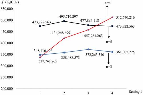
Finally, the single optimal solution for the five objective functions (total energy value, surface roughness, total noise, total cost, and carbon emission) was associated with the first parameter setting, and the number of roughing passes (n) equals 4. It is defined as follows: the total energy value is 495,965.751 Joule, surface roughness is 0.285 μm, total noise is 393.938 dBA, total cost is $ 288.587, and carbon emission is 337,748.265 $kgC{O}_2$. The values of the decision variables were suitable with $v_{r1}=50.003m/min$, $v_{r2}=50.020m/min$, $v_{r3}=50.005m/min$, $v_{r4}=50.005m/min$, $v_f=50.233m/min$, $f_{r1}=0.580mm/rev$, $f_{r2}=0.801mm/rev$, $f_{r3}=0.881mm/rev$, $f_{r4}=0.774mm/rev$, $f_f=0.101mm/rev$, $d_{r1}=3.000mm$, $d_{r2}=3.000mm$, $d_{r3}=2.000mm,d_{r4}=1.000mm$, $\mathrm{a}\mathrm{n}\mathrm{d}{d}_f=1.000mm.$ This result is the single optimal solution. It is good to be recommended according to the numerical example in this model.

If this solution is to be implemented in a real manufacturing process, it will need to be additional coded on the CNC machine. This will make the CNC machine smarter, because it can change machining parameters from one roughing pass to another. The values of the decision variables for the feed rate $\left(f\right)$ and depth of cut $\left(d\right)$ for the roughing pass tend to be close to the upper bond. The value of the feed rate is close to nine and the value of the depth of cut is close to three. This condition minimizes the processing time. In contrast, the values of the decision variables for the feed rate $\left(f\right)$ and depth of cut $\left(d\right)$ for the finishing pass tend to be close to the lower bound. The values of the feed rate and depth of cut are both close to one to keep the value of the surface roughness smaller than $6.3\text{mum}$.

4. Conclusions and future research

In this study, a multi-objective optimization model was developed by considering five objective functions that represent environmental, economic, and social factors. This paper proposed novel ideas for examining machining process time and machining power in detail. Additionally, the objective functions adopted in this study consider the total noise and cost of quality. Based on optimization performed using the Gamultiobj algorithm and TOPSIS method, a single optimal solution was identified for the first parameter setting value and four roughing passes (n) equals 4. The limitations of this paper are the firstly, the formulas for the total noise objective function are derived from regression equations with different CNC turning machines, and secondly, the parameters used in the numerical example are taken from some papers. So, for future research it should be considered such as a case study on one machine system, because the results will be different for other CNC turning machines. However, this proposed model can be a reference to be applied to different CNC turning machines.

Acknowledgements

This work was supported by the MR-UNS PNBP under Grant 452/UN27.21/PN/2020.

Disclosure statement

No potential conflict of interest was reported by the author(s).

Additional information

Funding

This work was supported by the MR-UNS PNBP [452/UN27.21/PN/2020].

Notes on contributors

Eko Pujiyanto

Eko Pujiyanto received the B.S. degree in Mathematics in 1993 and the M.Eng. degree in Industrial Engineering in 1998, both from Bandung Institute of Technology, Bandung and Ph.D. degree in Mechanical Engineering in 2012 from Gadjah Mada University, Yogyakarta, Indonesia. He is currently a member of The Center for Research in Manufacturing System at Sebelas Maret University. His main research is the modeling and experimentation of manufacturing processes. His research interests include modeling and optimization of sustainable manufacturing process using statistical and computational, and data analysis and optimization using heuristics. In addition to research in the field of sustainable manufacturing modeling, he is also experimental-based research related to biomaterials using the Taguchi Method. The results of the multi-response experiment using the Taguchi method were optimized simultaneously with the multi-objective optimization tool. He has authored/coauthored several papers on these subjects.

References

- Allwood, J. M., Cullen, J. M., & Milford, R. L. (2010). Options for achieving a 50% cut in industrial carbon emissions by 2050. Environmental Science & Technology, 44(6), 1888–27. https://doi.org/10.1021/es902909k
- Ameur, T. (2021). Multi-objective particle swarm algorithm for the posterior selection of machining parameters in multi-pass turning. Journal of King Saud University - Engineering Sciences, 33(4), 259–265. https://doi.org/10.1016/j.jksues.2020.05.001
- Arif, M., Stroud, I. A., & Akten, O. (2014). A model to determine the optimal parameters for sustainable-energy machining in a multi-pass turning operation. Proceedings of the Institution of Mechanical Engineers, Part B: Journal of Engineering Manufacture, 228(6), 866–877. https://doi.org/10.1177/0954405413508945
- Aungkulanon, P., & Luangpaiboon, P. (2016). Vertical transportation systems embedded on shuffled frog leaping algorithm for manufacturing optimisation problems in industries. SpringerPlus, 5(1), 1–25. https://doi.org/10.1186/s40064-016-2449-1
- Bagaber, S. A., & Yusoff, A. R. (2019). Energy and cost integration for multi-objective optimisation in a sustainable turning process. Measurement: Journal of the International Measurement Confederation, 136, 795–810. https://doi.org/10.1016/j.measurement.2018.12.096
- Banister, D. (2019). The climate crisis and transport. Transport Reviews, 39(5), 565–568. https://doi.org/10.1080/01441647.2019.1637113
- Bouzid, W. (2005). Cutting parameter optimization to minimize production time in high speed turning. Journal of Materials Processing Technology, 161(3), 388–395. https://doi.org/10.1016/j.jmatprotec.2004.07.062
- Chen, L. G., Li, P. L., Xia, S. J., Kong, R., & Ge, Y. L. (2022). Multi-objective optimization for membrane reactor for steam methane reforming heated by molten salt. Science China Technological Sciences, 65(6), 1396–1414. https://doi.org/10.1007/s11431-021-2003-0
- Chen, M. C., & Tsai, D. M. (1996). A simulated annealing approach for optimization of multi-pass turning operations. International Journal of Production Research, 34(10), 2803–2825. https://doi.org/10.1080/00207549608905060
- Cirtu, N. D., Dimitriu, R., Hartley, D., & Golder, A. A (1976). Survey of the noise levels of metal-cutting machine tools. Proceedings of the sixteenth international machine tool design and research Conference, 363–369. https://doi.org/10.1007/978-1-349-81544-9_50
- Costa, N., & Lourenço, J. (2017). Reproducibility of nondominated solutions. Chemometrics and Intelligent Laboratory Systems, 168, 1–9. https://doi.org/10.1016/j.chemolab.2017.07.002
- Deb, K., Pratap, A., Agarwal, S., & Meyarivan, T. (2002). A fast and elitist multi-objective genetic algorithm: NSGA-II. IEEE Transactions on Evolutionary Computation, 6(2), 182–197. https://doi.org/10.1109/4235.996017
- Du, F., He, L., Huang, H., Zhou, T., & Wu, J. (2020). Analysis and multi-objective optimization for reducing energy consumption and improving surface quality during dry machining of 304 stainless steel. Materials, 13(21), 1–26. https://doi.org/10.3390/ma13214693
- Eslami, Y., Dassisti, M., Lezoche, M., & Panetto, H. (2019). A survey on sustainability in manufacturing organisations: Dimensions and future insights. International Journal of Production Research, 57(15–16), 5194–5214. https://doi.org/10.1080/00207543.2018.1544723
- Faghiri, S., Aria, H. P., & Shafii, M. (2022). Multi-objective optimization of acetone droplet impingement on phase change material in direct-contact discharge method. Journal of Energy Storage, 46, 103862. https://doi.org/10.1016/j.est.2021.103862
- Hu, L., Liu, W., Xu, K., Peng, T., Yang, H., & Tang, R. (2019). Turning part design for joint optimisation of machining and transportation energy consumption. Journal of Cleaner Production, 232, 67–78. https://doi.org/10.1016/j.jclepro.2019.05.297
- Hwang, C.-L., Lai, Y.-J., & Liu, T.-Y. (1993). A new approach for multiple objective decision making. Computers & Operations Research, 20(8), 889–899. https://doi.org/10.1016/0305-05489390109-V
- Jayal, A. D., Badurdeen, F., Dillon, O. W.,sJr., & Jawahir, I. S. (2010). Sustainable manufacturing: modeling and optimization challenges at the product, process and system levels. CIRP Journal of Manufacturing Science and Technology, 2(3), 144–152. https://doi.org/10.1016/j.cirpj.2010.03.006
- Jiang, Z., Gao, D., Lu, Y., & Liu, X. (2019). Optimization of cutting parameters for trade-off among carbon emissions, surface roughness, and processing time. Chinese Journal of Mechanical Engineering, 32(1), 1–18. (English Edition). https://doi.org/10.1186/s10033-019-0408-9
- Kallio, S., & Siroux, M. (2021). Exergy optimization of a multi-stage solar micro-cogeneration system. IET Renewable Power Generation, 1–12. https://doi.org/10.1049/rpg2.12372
- Khalilpourazari, S., Khalilpourazary, S., Çiftçioğlu, A. Ö., & Weber, G. (2020). Designing energy-efficient high-precision multi-pass turning processes via robust optimization and artificial intelligence. Journal of Intelligent Manufacturing, 321, 1621–1647. https://doi.org/10.1007/s10845-020-01648-0
- Li, C., Tang, Y., Cui, L., & Yi, Q. (2013). Quantitative analysis of carbon emissions of CNC-based machining systems. 10th IEEE international conference on networking, sensing and control, 869–874. https://doi.org/10.1109/ICNSC.2013.6548852
- Liu, Z. J., Sun, D. P., Lin, C. X., Zhao, X. H., & Yang, Y. (2016). Multi-objective optimization of the operating conditions in a cutting process based on low carbon emission costs. Journal of Cleaner Production, 124, 266–275. https://doi.org/10.1016/j.jclepro.2016.02.087
- Lu, L., & Anderson-Cook, C. M. (2013). Adapting the Hypervolume Quality Indicator to Quantify Trade-offs and Search Efficiency for Multiple Criteria Decision Making Using Pareto Fronts. Qual. Reliab. Engng. Int, 29, 1117–1133. https://doi.org/10.1002/qre.1464
- Lu, C., Gao, L., Li, X., & Chen, P. (2016). Energy-efficient multi-pass turning operation using multi-objective backtracking search algorithm. Journal of Cleaner Production, 137, 1516–1531. https://doi.org/10.1016/j.jclepro.2016.07.029
- MATLAB. (2020). Version 9.8 (R2020a). Natick, Massachusetts: The MathWorks Inc.
- Nur, R., Kurniawan, D., Noordin, M. Y., & Izman, S. (2015). Optimizing power consumption for sustainable dry turning of treated aluminum alloy. Procedia Manufacturing, 2, 558–562. https://doi.org/10.1016/j.promfg.2015.07.096
- Olaru, S. C., Slǎtineanu, L., Silitrǎ, M., Mihalache, A. N., & Coteatǎ, M (2017). Investigation of the sound intensity level in the case of a universal lathe. MATEC Web of Conferences, 112, 1–6, https://doi.org/10.1051/matecconf/201711201025
- Pangestu, P., Pujiyanto, E., & Rosyidi, C. N. (2021). Multi-objective cutting parameter optimization model of multi-pass turning in CNC machines for sustainable manufacturing. Heliyon, 7(2), e06043. https://doi.org/10.1016/j.heliyon.2021.e06043
- Pawanr, S., Garg, G. K., & Routroy, S. (2019). multi-objective optimization of machining parameters to minimize surface roughness and power consumption using TOPSIS. 7th CIRP Global Web Conference, Procedia CIRP 86, 116–120. https://doi.org/10.1016/j.procir.2020.01.03
- Pawanr, S., Garg, G. K., & Routroy, S. (2021). Modelling of variable energy consumption for CNC machine tools. Paper Presented at the Procedia CIRP, 98, 247–251. https://doi.org/10.1016/j.procir.2021.01.038
- Perdomo, I. L. F., Quiza, R., Haeseldonckx, D., & Rivas, M. (2020). Sustainability-focused multi-objective optimization of a turning process. International Journal of Precision Engineering and Manufacturing - Green Technology, 7(5), 1009–1018. https://doi.org/10.1007/s40684-019-00122-4
- Phadke, M. S. (1989). Quality engineering using robust design (pp. 40–50). Prentice Hall.
- Rao, R. V., & Kalyankar, V. D. (2013). Multi-pass turning process parameter optimization using teaching-learning-based optimization algorithm. Scientia Iranica, 20(3), 967–974. https://doi.org/10.1016/j.scient.2013.01.002
- Schultheiss, F., Johansson, D., Bushlya, V., Zhou, J., Nilsson, K., & Ståhl, J. (2017). Comparative study on the machinability of lead-free brass. Journal of Cleaner Production, 149, 366–377. https://doi.org/10.1016/j.jclepro.2017.02.098
- Sellami, A., Ali, M. B., & Kairouani, L. (2020). Pareto-optimization of msf-ot/tvc desalination plant using surface response methodology and genetic algorithm. Desalination and Water Treatment, 204, 10–21. https://doi.org/10.5004/dwt.2020.26229
- Shin, S. M., Kim, Y. M., & Meilanitasari, P. (2019). A holonic-based self-learning mechanism for energy-predictive planning in machining processes. Processes, 7(10), 739. https://doi.org/10.3390/pr7100739
- Ståhl, J. E., Schultheiss, F., & Hägglund, S. (2011). Analytical and experimental determination of the ra surface roughness during turning. Procedia Engineering, 19, 349–356. https://doi.org/10.1016/j.proeng.2011.11.124
- Tian, C., Zhou, G., Zhang, J, & Zhang, C. (2019). Optimization of cutting parameters considering tool wear conditions in low-carbon manufacturing environment. Journal of Cleaner Production, 226, 706–719. https://doi.org/10.1016/j.jclepro.2019.04.113
- Yi, Q., Li, C., Tang, Y, & Chen, X. (2015). Multi-objective parameter optimization of CNC machining for low carbon manufacturing. Journal of Cleaner Production, 95, 256–264. https://doi.org/10.1016/j.jclepro.2015.02.076
- Zhang, H., Deng, Z., Fu, Y, Lv, L., & Yan, C. (2017). A process parameters optimization method of multi-pass dry milling for high efficiency, low energy and low carbon emissions. Journal of Cleaner Production, 148, 174–184. https://doi.org/10.1016/j.jclepro.2017.01.077
- Zhang, Z., Tang, R., Peng, T., Tao, L., & Jia, S. (2016). A method for minimizing the energy consumption of machining system: integration of process planning and scheduling. Journal of Cleaner Production, 137, 1647–1662. https://doi.org/10.1016/j.jclepro.2016.03.101
- Zhong, Q., Tang, R., & Peng, T. (2017). Decision rules for energy consumption minimization during material removal process in turning. Journal of Cleaner Production, 140, 1819–1827. https://doi.org/10.1016/j.jclepro.2016.07.084