A review of response surface methodology for biogas process optimization

Abstract

This paper aimed at reviewing current researches on the use of Response Surface Methodology in the optimisation of Biogas processes. It explored the performance of RSM in biogas process optimization, the most effective technique and the attendant effective software used in such processes. It attempted to review literature in the area. 55 articles were systematically reviewed. The online databases included were Google Scholar, Scopus and other statistics-based optimization research databases with keywords from Response Surface Methodology in Biogas Optimization. The review finds that RSM proves to be an effective statistical tool. It has achieved optimum objectives for biogas production: increased biodegradability, optimum biogas yield and methane production, increased Total Solid and reduced Volatile Solids and an increased COD removal. The key advantage of RSM was found to be a reduced number of experimental trials, making it time and cost-effective. 37 process parameters have been optimised using RSM, over the last two decades. Five of these parameters are dominant. Namely,: Temperature, pH, Retention time, Pre-treatment and Loading rate. The major challenges associated with the use of RSM in biogas production process optimization are the limited experimental range. Techniques to combine RSM with other optimization methods such as the Taguchi, Kriging or the Artificial Neural Network (ANN) are being developed to address these challenges. Design Expert software is the most used software because of its low cost of use. However, Statistica offers a better efficiency.

Keywords:

• biogas optimization
• response surface methodology
• review
• anaerobic digestion

PUBLIC INTEREST STATEMENT

As the world moves towards renewable energies for a more sustainable environment, diverse clean energy resources are being utilised. One of these is biogas, generated through anaerobic digestion. Biogas is obtained from organic materials, thus biogas generation is not only a good source of energy but also a waste management technique. However, as any other biological process, anaerobic digestion does not reach its maximum potential. This is why for decades; scientists and researchers have been working on mechanisms that would result in optimum biogas production. Various optimisation methods and techniques have been developed over the years. One of these techniques is the Response Surface Methodology (RSM). The Response Surface Methodology is a five-step method developed to study the impact of factors on a specific variable and to estimate the optimum condition. It is from this background that the authors decided to review this optimization method.

1. Introduction

For centuries, fossil fuel has been the world’s main source of energy. However, due to the emission of greenhouse gases (GHGs), one of the main causes of global warming, the negative impact of fossil fuel use outweighs its benefits (Bessou et al., 2011). GHG emissions, coupled with other problems such as environmental pollution (related to the use of fossil fuel), increased consumption, declining land fertility, inefficient waste management, and deforestation which are the results of mismanagement of natural resources all over the globe, have enjoined the United Nations (UN) to put in place measures to mitigate them (Mkruqulwa et al., 2019; Nevzorova & Karakaya, 2020). The seventeen (17) Sustainable Development Goals (SDGs) aim at ensuring a better and a sustainable future for the world. Goal seven (7) focuses on the energy sector; it aims at achieving global access to clean and affordable electricity by 2030 (United Nations, 2015). Energy access is crucial for food production, security, increased financial income, health and climate change.

Renewable energies, example, hydropower, solar power, wind power, and biofuel are the main interests of the future energy sector (Mkruqulwa et al., 2019). Biogas production is most likely to be preferred, not only because of its advantages in terms of cleanliness and sustainability but also because it is produced from organic waste and therefore, it does not result in loss of food or biodiversity (Balat & Balat, 2016; Vasavan et al., 2018). Biogas can be an important component of the solution to meet the goals of the United Nations for sustainable development (Memon & Memon, 2020). It can be used to generate electricity and reduce greenhouse gas emissions. Biogas is a combination of methane (CH₄), carbon dioxide (CO₂) and hydrogen sulphide (H₂S), ammonia (NH₃), hydrogen (H₂) and minor amounts of other gases such as carbon monoxide (CO), nitrogen (N₂) and oxygen (O₂; Anunputtikul & Rodtong, 2004; Jorgensen, 2009; Mkruqulwa et al., 2019). Biogas is produced by a biological process called anaerobic digestion (AD).

Anaerobic digestion, as defined by (Mukumba et al., 2016) and (Abdeshahian et al., 2016), is a biological process that takes place in the absence of oxygen and results in the production of methane through the decomposition of biomass. Biomass which is considered as an organic matter, is a biodegradable portion of materials such as agriculture residues (vegetal and animal), forest residues and waste (industrial and municipal; Umana et al., 2020). Organic materials are made up of carbon, oxygen, hydrogen and nitrogen (Umana et al., 2020). Anaerobic digestion is a good technology for waste management because it maximizes energy production and minimizes the cost of treatment of organic materials (municipal solid waste, food waste, animal manure, agricultural residues, sewage, industrial waste and human excrement; Abdeshahian et al., 2016; Shen et al., 2015). It is also a great solution to wastewater pollution which is one of the most important environmental problems in the world today (Buaisha et al., 2020).

The third law of thermodynamics, however, states that no system has 100% efficiency. This explains why for centuries, humanity has been working to increase the efficiency of chemical and biochemical processes (to achieve 100% efficiency). In that attempt, “process optimization” techniques have been generated. Process optimization has significant importance in industrial processes and it is a well-accepted part of any industry, especially biotechnological firms where the slightest change in a production process can have a significant impact on the product (Reddy et al., 2008).

Since the discovery of biogas, there have been several pieces of research and experiments to improve the efficiency of anaerobic digestion. These studies have led to improvements in both production process and biogas quality (methane content increment and GHG reduction; Enitan-folami et al., 2016). The process of optimising the biogas production parameters is complex due to the many interactive effects of these parameters (Sathish & Vivekanandan, 2016). Response surface methodology (RSM), for instance; a mathematical and statistical set of techniques used to both design and build empirical models, examine the impact of the inputs and estimate the optimal conditions is one such method (Muthuvelayudham et al., 2006; Rastega et al., 2011; Sarabia & Ortiz, 2009). The purpose of RSM is to maximize a response (dependent variable) affected by several input variables (independent variables; Bradley, 2009).

In an attempt to obtain maximum efficiency in biological processes, various optimisation methods and techniques have been developed over the years. One of these techniques is the Response Surface Methodology (RSM). The Response Surface Methodology is a five-step method developed to study the impact of factors on a specific variable and to estimate the optimum condition. Several parameters such as temperature, pre-treatment, pH can impact biogas production, thus, could be adjusted to optimize the quantity and quality of biogas. This research reviews current research on the use of Response Surface Methodology in the optimisation of Biogas processes. It explores the performance of RSM in biogas process optimisation; the most effective technique/methodology and the attendant effective software used in such processes. A total of 55 articles, published from 2000 to 2022, were systematically reviewed and included in the database.

2. Methodology

The study was guided by the process of bibliometric studies outlined by Akpoti et al. (Akpoti et al., 2019). The literature database on Response Surface Methodology in Biogas optimization was developed through a systematic search in online databases (using Google Scholar and Scopus). A Boolean search by keywords and phrases were used to query through scientific research engines and platforms. Initial search includes strictly biogas process parameters optimization. Then we enlarged the database to statistical-based optimization research that includes Response Surface Methodology. Keywords and expressions included biogas, process parameters, optimization and Response Surface Methodology. All articles dealing with optimization of biogas process parameters through response surface methodology from site-specific, sub-regional, country level to global were included in the database. Each article was reviewed and the database was organized according to the pre-established checklist to collect metadata (Table 1). The approach included all “relevant” publications between the period 2000 and 2021. However, we referred to a few articles prior to the year 2000 that are important to understanding concepts or methods. We intentionally excluded the theoretical and mathematical formulations of the methods reported in the papers assessed for readability and easy understanding. In total, 55 articles were systematically reviewed and included in the database. These papers concerned solely those published between 2000 and 2021. A systematic review was conducted on the collected data (Figure 1), and results are presented and discussed.

Figure 1. Methodology adapted in this article.

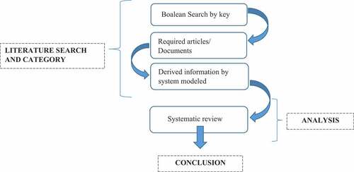
Table 1. Checklist of meta-data for systematic review (adapted from (Akpoti et al., 2019))

Items	Definition
Title	Title of the article or document under review
Objective	Objective of the study
Methodology	Method used to meet the study objective
Process parameters	Process parameters considered for optimization
Keys notes/summary	Important findings from the study and limitations
Criteria Software/Computer program	Information on model implementation and different software used
Authors	Author(s)
Document type	Journal article, book chapter, conference paper, etc.

3. Results and discussion

3.1. Concept of response surface methodology

Response surface methodology (RSM) is a mathematical and statistical set of techniques used to both design and build empirical models, examines the impact of the inputs and estimates the optimal conditions (Bradley, 2009; Muthuvelayudham et al., 2006; Rastega et al., 2011). It was pioneered in 1951 by Box and Wilson (Box & Wilson, 1951), to imitate experimental responses through second-degree polynomial (quadratic) models (Bashir et al., 2015; Bradley, 2009). RSM is designed to optimize a response that is affected by multiple variables (Montgomery, 2017).

Considering two independent variables (x₁ and x₂) and an output or response variable (y; equation 1(Equation\,1) $y=f\left(x_1,x_2\right)+\epsilon$(Equation\,1) ), the response (y) will depend on the two variables (x₁ and x₂):

(Equation\,1) $y=f\left(x_1,x_2\right)+\epsilon$(Equation\,1)

$\epsilon$ is the error margin that could be observed in response y. Hence, the response surface is the surface represented by equation 2(Equation\,2) $\eta =f\left(x_1,x_2\right)$(Equation\,2) below:

(Equation\,2) $\eta =f\left(x_1,x_2\right)$(Equation\,2)

With $\eta ,$ the response surface area and $x_1,x_2$, two independent variables.

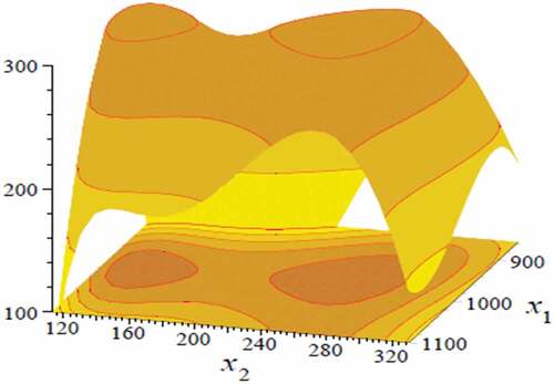
The response surface is represented graphically most of the time, either as contour plots or in a three-dimensional space (Bradley, 2009; Montgomery, 2017). Figure 2 indicates a typical representation of a response surface. RSM is applied for optimising process parameters in many field areas (chemical, biochemical, material science, wastewater treatment, etc.; Alikunju et al., 2017; Bashir et al., 2015; Beevi et al., 2014; H. B. Nielsen et al., 2007; Jung et al., 2015).

Figure 2. A graphical representation of an RSM response (Bradley, 2009).

A study by Bashir et al. (Bashir et al., 2015) found that 352 out of 3190 articles related to RSM application in optimizing process parameters in the different research areas (Chollom et al., 2019); with nearly ten (10) times increase in the number of articles were published between 2000 and 2013. This agrees with Aydar (Aydar, 2018) that RSM is one of the most popular analytical methods for optimization. In recent times, RSM has been used in several industries to optimize process parameters and to study the dynamic effects of input variables in biochemical and chemical reactions(Chelladurai et al., 2020). Breig and Luti (Breig & Luti, 2021) reviewed the application of response surface methodology in microbial cultures and conclude that: in addition to offering the possibility of investigating the parameters that affect the response and illustrating the relative magnitude and interactions between them, RSM is a very useful tool for determining the optimal conditions for increasing microbial production and for building mathematical models that predict the output variable as a function of combinations of parameter levels. RSM is a very useful tool.

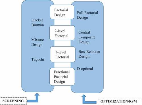
RSM, as illustrated by Figure 2, is a multi-stage method, which uses experimental designs for fitting first-order or second-order polynomial models (Bartz-Beieslstein et al., 2010). The most important step of RSM is the Design of Experiments (DoE). The success of the mathematical model for the correctness of the response surface construction is highly dependent on the selection of experimental design (Aydar, 2018). The DoE also aims at finding the variables with a higher impact on the response (in cases where the number of input variables is considerable; Aydar, 2018). Makela, in his review study, defined the experiment design (or design of experiment) as “a collection of tools used for studying the behavior of a system” (Makela, 2017). RSM is a combination of experimental designs and a strategy to develop a new dataset by first- or second-order polynomial equations in a systematic test method (Ramaraj & Unpaprom, 2019). RSM analysis is predominantly done with symmetrical experimental designs which are Doehlert Design (DD), Central Composite Design (CCD), the Box-Behnken Design (BBD), and a three-level full factorial design (Bezerra et al., 2008). Each of the experimental designs has its advantages and limits (Chollom et al., 2019).

RSM offers an advantage over traditional optimization methods concerning the number of experiments and the multifactorial interactivities over a response (Tetteh et al., 2017). Two other advantages of RSM are that: by allowing the identification of optimal conditions, RSM offers an assessment of the sensitivity of these optimum conditions to the variations of the experimental variables it quantifies the response-input variable relationship (Kilickap, 2010) and the possibility of making projections, which allow visual interpretations of that relationship (Rastega et al., 2011). The greatest advantage of RSM remains the time and cost savings due to the reduced number of experimental trials (Boyaci, 2005).

However, Bas and Boyaci (Bas & Boyaci, 2007) revealed the main limitation of RSM, namely its confinement to fitting the data to a second-order polynomial equation. Some complex data are not compatible with a second-order polynomial model. Breig and Luti (Breig & Luti, 2021) confirmed the challenge identified by Bas and Boyaci, and pointed at two other disadvantages in using RSM, which are: the limited experimental range of this methodology and the need to use the steepest descent technique to transfer the optimal area to supply the combinations of parameters when doing the preliminary approximation of parameters. Techniques for merging RSM and other optimization methods are being studied in order to overcome the challenges stated above (Breig & Luti, 2021).

3.2. Steps of response surface methodology

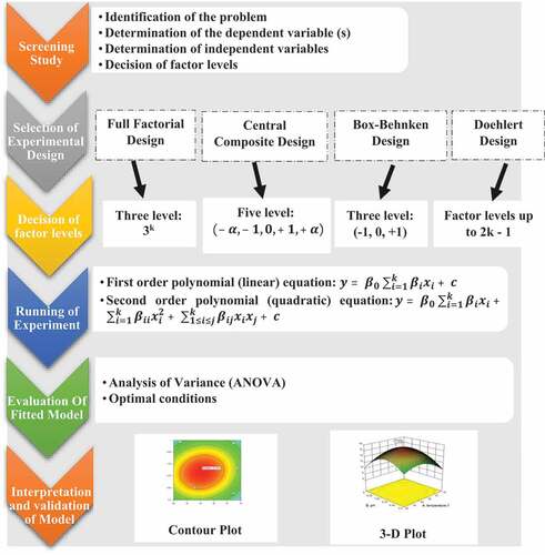
The response surface methodology is a statistical procedure for optimizing one or more responses affected by more than one factor (independent variable). RSM is based on surface placement, therefore, its success depends solely on understanding the topography of the response surface (e.g., maximum local, minimum local and ridgelines) and being able to identify the area where the optimal condition occurs (Bradley, 2009). It is a strong tool for process optimization, as it has been used to evaluate the overall effect of various factors on process parameters various fields of study: clinical and biological sciences, social sciences, nutrition sciences, physics and engineering sciences. The methodology is a heuristic optimization, meaning there is no certainty of reaching the optimal response in a finite time during an RSM optimization process (Bartz-Beieslstein et al., 2010). RSM, however, as mentioned earlier, follows specific steps to arrive at the desired result. Figure 3 presents these different steps while this section discusses them.

Figure 3. Steps of response surface methodology.

3.2.1. The screening study

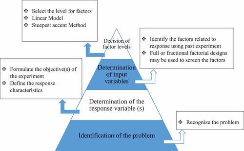
The screening study, as shown in Figure 4, consists of the identification of the problem, the determination of the response variable (s), the determination of input variables, and the decision of factor levels (Figure 4; Ranganath, 2015). After the determination of the response (s) and its input variables, the level of influence of each of the variables on the response(s) is estimated using linear and quadratic models such as full factorial or fractional factorial designs (Olivero et al., 1998).

Figure 4. Steps of the screening process.

Independent variables or factors are the variables that are subject to manipulations in order to study their impact on a specific response. The factor levels represent the number of settings of the factor that is considered in the experiment; they are the different values that the factor can assume (Bezerra et al., 2008). For example, an experiment to investigate the impact of pH on fermentation, where five (5) different pH values were considered; here pH is a factor and its five (5) values are the factor levels.

3.2.2. Selection of experimental design

According to the definition of Montgomery (Montgomery, 2017), a Statistical design of experiments refers to the planning process of the experiment in order to collect appropriate data and analyse them by statistical methods, allowing valid and objective conclusions to be drawn. The main purpose of the DoE is to find appropriate experimental designs, by selecting the points where the response will be monitored (Bradley, 2009). Montgomery (Montgomery, 2017) lists several desirable features to consider when deciding on a design for a response surface. The choice of an experimental design depends mostly on:

• The type of variables (quantitative or qualitative)

• The type of experiment (process or mixture)

• The number of variables

• The range of the study

• The limitations of the variables

A number of experimental designs exist (Figure 6), but only four are mostly used in RSM, namely: Central Composite Design (CCD), Box-Behnken Design (BBD), Full Factorial, and Optimal Designs. The choice of designs is also based on the required experimental points and the numbers of runs (Breig & Luti, 2021) As shown in Figure 5, the Central Composite Design (CCD) is the most used design followed by the Box-Behnken Design (BBD), then the Full Factorial and Optimal Designs. This section will discuss each of these experimental designs.

Figure 5. Proportional distribution of the experimental designs used in the articles read.

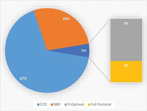
Figure 6. List of experimental designs.

4. The central composite design (CCD)

Also known as the Box-Wilson central composite design, it is the most commonly used experimental design for fitting polynomial equations (Montgomery, 2017). CCD is made up of a three-level factor (two-level full or fractional factorial design and a central point which is the middle level) augmented by a star point denoted $\alpha$ increasing the factor levels to 5 (Olawoye, 2016; Witek-Krowiak et al., 2014). The star point gives more flexibility to the experimental design by estimating the curvature (Nnaemeka et al., 2022; Nooraziah & Tiagrajah, 2014; Yılmaz & Şahan, 2020).

Even though CCD requires fewer runs than the full factorial design (FFD), it gives the same amount of information (Witek-Krowiak et al., 2014). Depending on the position of the star points, three different types of central composite designs are distinguished:

• The Circumscribed Central Composite (CCC) where the star points are located outside the experimental domain. CCC requires five levels per factor and is a rotatable design (the variance of response at any point is only dependent on the distance between that point and the center point) Handbook of Statistical Methods, 2013). Rotatability is also called iso-variance per rotation (Ait-Amir et al., 2015).

• The Inscribed Central Composite (CCI) is regarded as a CCC design reduced to fit within the experimental domain (Ait-Amir et al., 2015). It is used in situations where there are limits on factor levels; thus, it requires the same number of factor levels as CCC design and each factor level is by $\alpha$ Central Composite Designs (CCD), 2013). CCI is both rotatable and orthogonal.

• The Face-Centred Composite (CCF): star points are located at the middle of each face of the experimental domain with $\alpha =\pm 1$ (Ait-Amir et al., 2015). It requires three-factor levels and is an orthogonal design (the effect of any factor across the experimental domain, nullifies the effects of the other factors) Handbook of Statistical Methods, 2013).

According to Witek-Krowiak et al. (Witek-Krowiak et al., 2014), to choose the right type of CCD, it is very important to consider the region of operation and the region of interest. Table 2 describes the characteristics of the various CC designs where $N_f$, $N$ and $k$ are the numbers of trials per fractional factorial experiments, the total number of trials, and the number of factors, respectively.

Table 2. Characteristics of the CC designs

Type of Central Composite Design	Rotatability	Number of points at the center	$\alpha$	Experiment
Circumscribed	Rotatable	1	$\alpha =\sqrt[4]{N_f}$
Face-centered	Orthogonal	1	$\alpha =\sqrt{\frac{\sqrt{N_f\times N}-N_f}{2}}$
Inscribed	Rotatable and orthogonal	$\sqrt[4]{N_f}+4-2k$	$\alpha =\sqrt[4]{N_f}$

5. The box-behnken design (BBD)

BBD was created in 1960 by Box and Behnken as a replacement to the FFD, which required a large number of experiments (Witek-Krowiak et al., 2014). BBD is, therefore, more economical and more efficient than FFD especially when it comes to large experimental numbers (Bezerra et al., 2008) and slightly more labor efficient than CCD. The experimental points of BBD are located on a hypersphere halfway from the center point which offered it the advantage of pointing out the limits of the experimental boundaries (Bezerra et al., 2008; Ramaraj & Unpaprom, 2019).

The two major challenges with BBD are that it can only be used to fit the quadratic model and take a minimum of three-factor levels (Ramaraj & Unpaprom, 2019; Witek-Krowiak et al., 2014). BBD can be rotatable or near rotatable when there are more than three-factor levels and if points are added at the center (Ait-Amir et al., 2015; Guthrie et al., 2013).

6. The full factorial design (FFD)

Even though it is less used as compared to the CCD and the BBD, the full factorial design is one of the most common designs. This design only works with a minimum of two (2) and a maximum of five (5) independent variables (Bradley, 2009; Leiviska, 2013) because it requires a high number of experiments (Bezerra et al., 2008). The large number of experiments required is because the design takes into consideration all possible interactions between the factors (Witek-Krowiak et al., 2014). Although FFD can only fit second-order polynomials, Khattree and Rao (Khattree & Rao, 2003a) affirmed that it may have problems fitting second-order and higher models. Box and Behnken created the central composite design to counter the cost and time limitations related to FFD.

7. Optimal designs

Optimal design matrices are a non-orthogonal set of computer-based experimental designs which are used in cases where the other factorial and fractional factorial designs cannot be applied (Leiviska, 2013) and are distinguished by adding by the addition of alphabetical prefix:

• D-optimality design

• E-optimality design

• G-optimality design

• V-optimality design

• I-optimal design

• T-optimal design

In this paper, the D-optimal design is discussed. It is the most used optimal design (Atkinson & Fedorov, 1975; Khattree & Rao, 2003a; Rockafellar, 2015; Simons & Chernoff, 1976). Most optimal designs deal with the proper value of the matrix $X^{T}X$. The “D” in D-optimal stands for “Determinant”. That is, in the D-optimal design, the objective is to maximize the determinant $X^{T}X$ (De Aguiar et al., 1995; Bradley, 2009; Copelli et al., 2018) and minimize the variance of the parameters.

The advantage of the D-optimal design is that it can be used for any experimental purpose (screening, RSM), it can fit any model (first-order, second-order, cubic), and it works with a large number of experimental runs (“D-Optimal designs,” 2013). Table 3 below, summarizes the different experimental design characteristics.

Table 3. Different experimental designs and their characteristics

Experimental Design	Characteristics
DOEHLERT DESIGN	It allows a sequential approach to the response surface It simplifies the study of a restricted zone by changing the dimensions of the initial simplex It is associated with the loss of information due to alignments in the area	k is the factor number of the central point $c_p$ is the replicate number of the central point
OPTIMAL DESIGN	It is important when the experimental cost is high or there are constraints on factor settings It requires fewer runs than standard factorial designs The design space is constrained
FFD	It has an unrestricted number of factors and factor levels It is labor-intensive It is the most secured design
BBD	It can accommodate a minimum of three (3) factors It has 3 levels of factors (upper level, lower level, center point) It requires several experiments according to $N=2k\left(k-1\right)+c_p$ All levels of factors should be set only at three levels (−1, 0, +1) with equidistant intervals between these levels
CCD	It can accommodate a minimum number of two (2) factors It has five (5) levels of factors It requires an experiment number according to $N=k^2+2k+c_p$, All its factors are studied in five levels $\left(-\alpha ,-1,0,+1,+\alpha \right)$ It involves three types of composite designs (Circumscribed, face-centered, and inscribed)

7.0.3. Running of experiment

An experiment as defined by the Design Institute for Six Sigma (Hromi, 1957) is a procedure or analysis that results in the acquisition of data. After the input variables are found and the experimental design is selected, experiments must be planned. Experiments are very important; therefore, they have to be rationally planned (Olivero et al., 1998). The number of experiments depends on the type of experimental design selected (refer to Table 7). In microbial production, experiments are run in replicates for more precision and accuracy.

Table 4. Examples of optimum temperature

Substrate	Optimum Temperature	Optimum Response	Reference
Biomass from cassava and solid waste from vineyards	35 °C ± 0.5	346.28 mL CH4/g VS added	(Mkruqulwa et al., 2019)
Corn ethanol distillery wastewater	37 °C	551 mL CH4 g-1 VS added	(Gyenge et al., 2014)
Grass silage	37.3 °C	3410.25 CC	(Alfarjani et al., 2013)
Poultry dropping and pawpaw peels	36.84 °C	3991.77 10^−4 m^3/VS	(Dahunsi et al., 2016)
Rice straw	50 °C	0.72 m^3 biogas yield	(Sathish & Vivekanandan, 2014)
Co-digestion of Prosopis juliflora seeds, water hyacinth, dry leaves, and cow manure	35.557 °C	Actual methane yield (AMY) of 396.0 ± 6 L/kgVS, anaerobic biodegradability of 76.6%, and the TS reduction of 41.1%	(Vijin Prabhu et al., 2021)
Tannery wastewater	35.5–37 °C	200–217 mL biogas/g VS 108–118 mL CH4/g VS 69–74% VS, 54–57% TS 47–48% COD reduction	(Mpofu & Oyekola, 2019)
Waste food materials	44.03 °C	80% of CH4	(Pati et al., 2019)
Green algae	37 °C	346 ml biogas yield	(Zaidi et al., 2019)
Dairy effluents	35 °C	40% sludge ratio, with the removal of 47.7% volatile solids and 266.5 ml per gram of removed volatile solids	(Nouri et al., 2020)

Table 5. Examples of optimum pH

Substrate	Optimum pH	Optimum Response	Reference
Secondary Tannery sludge (STNS)	6.5–6.6	200–217 mL biogas/g VS 108–118 mL CH4/g VS 69–74% VS, 54–57% TS 47–48% COD reduction	(Mpofu & Oyekola, 2019)
Liquid swine manure and sugar beet molasses	5.32	31.9 L/d biogas production rate o 29.33% hydrogen content 1.52 mol-H2/mol-sugar hydrogen yield	(Wu et al., 2013)
De-oiled jatropha	6.5	307.4 ± 4.5 mL H2 cumulative hydrogen production	(G. G. Kumar et al., 2014)
Slaughterhouse wastewater (SWW)	6.84	85.03 and 72.10% Maximum TOC and TN removals 19.54 mg/L minimum TSS residual 116.56 mL/min maximum biogas yield	(Bustillo-lecompte & Mehrvar, 2017)
Flower waste	7.2	Highest biogas yield of 568 ml CH4/g Vs	(Gopal et al., 2021)
Co-digestion of Prosopis juliflora seeds, water hyacinth, dry leaves, and cow manure	7.034	Actual methane yield (AMY) of 396.0 ± 6 L/kgVS, anaerobic biodegradability of 76.6%, and the TS reduction of 41.1%	(Vijin Prabhu et al., 2021)
Co-digestion of waste food materials and cow dung	7.02	The response at the optimum conditions is 17.33 ml	(Pati et al., 2019)
Rice Straw	7.5	The highest level of biogas 0.72 m3	(Sathish & Vivekanandan, 2014)

Table 6. Optimum hydraulic retention times

Substrate	Optimum Hydraulic Retention Time	Optimum Response	Reference
SWW	15 h	5,800 mL/d biogas production 80.8% COD removal	(Chollom et al., 2019)
High-load compost leachate	46 h	84 % COD removal 76 mL/mg h biogas production rate	(Elyasi et al., 2015)
Wastewater from the bagasse-based pulp and paper industry	23 h	84.3% COD removal 230.9 mg/l h COD removal rate 21.2 l/d biogas production	(Taylor et al., 2015)
Volatile fatty acids	22 h	102 mL/L/h biogas production rate	(Amani et al., 2012)
Co-Digestion of Food Waste with Sewage Sludge	38.8 days	16% increase in biogas yield of 81.5% COD efficiency 69.2% VS efficiency	(Abdul Aziz et al., 2022)
Starchy sediment	30 days	403 ml/g TVS of biogas added 65.07% TVS removal	(Srivichai & Thongtip, 2021)
Corn-chaff and cow dung digestate	37 days	Highest biogas yield of 6.19 L	(Iweka et al., 2021)

Table 7. Examples of optimum pre-treatment conditions

Substrate	Pre-treatment Type	Optimum Pretreatment Conditions	Optimum Response	Reference
The organic fraction of municipal solid waste (OFMSW)	Biological Thermochemical	4.72 g/L NaOH dose 180 °C temperature 30.3 min pre-treatment time	169.5% enhanced biogas yield	(Bala & Mondal, 2019)
Excess sludge	Alkaline Mechanical	11.8 pH 21 days SRT	64, 84% Reduction in volatile solids 78.5% reduction in proteins and carbohydrates 15% enhanced gas production	(Murugan & Sivasamy, 2016)
Waste activated sludge	Photo-Fenton	725 g H2O2/kg TS 80 H2O2/Fe^2+ molar ratio 40 min irradiation time	75.7% total VS reduction 81.5% COD removal 0.29–0.31 m3/kg VSfed.d biogas production rate	(Heng et al., 2017)
Food waste	Alkaline, ultrasonication And thermal	pH 9 alkalinepre-treatment at 130 °C for 50 min Thermal pre-treatment 30 min ultra-sonication pre-treatment	The production of biogas increased by 100% with full utilisation of the COD in 25 days, with no significant downtime	(Menon et al., 2016;
Asparagus Stover	Alkaline	19d pre-treatment time 4.2%NaOH concentration 74 g dose of water	277.86 mL/g VS biogas yield	(Sun et al., 2017)

7.0.4. Selection of model

The response function (f) largely depends on the nature of relationship between the response and the independent variables and the class of experimental design selected must fit an experimental model. In the application of RSM in practice, it is required to build an experimental model for the actual response surface. The model is built on the actual data of the process or system and is a regression model (empirical model; Sarabia & Ortiz, 2009). A regression model uncovers the relationships between the response and the set of independent variables in a fixed data set and predict the optimal response to different combinations of the process variables (Nor & Wan, 2020). Regression models are generated using the least square method which is a multiple linear regression which minimizes the sum of squares distances between the actual and the predicted data (Nor & Wan, 2020; Sarabia & Ortiz, 2009).

Two types of experimental models are used in response surface optimization: the first-order multiple linear model or orthogonal model which is used when there are two independent variables as formulated in Equation 3(Equation\,3) $y=\hspace{0.17em}{\beta }_0+{\beta }_1{x}_1+{\beta }_2{x}_2$(Equation\,3) :

(Equation\,3) $y=\hspace{0.17em}{\beta }_0+{\beta }_1{x}_1+{\beta }_2{x}_2$(Equation\,3)

Where y is the response and $x_1$ and $x_2$ are the independent variables. This model only fits a 2-level Factorial and reduces the variance of the regression factors. However, most times, the curvature of the response surface is so strong that a first-order model is not adequate. Thus, the need for a second-order multiple linear model or quadratic model, which is the most, used in RSM problems. Equation 4(Equation\,4) $y={\beta }_0+\sum ki=1{\beta }_i{x}_i+\sum ki=1{\beta }_{ii}{x}_i^2+\sum ki=1\sum ki=2{\beta }_{ij}{x}_i{x}_j$(Equation\,4) presents a second-order model with k-independent variables (regressors) and β set of unknown parameters.

(Equation\,4) $y={\beta }_0+\sum ki=1{\beta }_i{x}_i+\sum ki=1{\beta }_{ii}{x}_i^2+\sum ki=1\sum ki=2{\beta }_{ij}{x}_i{x}_j$(Equation\,4)

Second-order models are more flexible. They can fit Central Composite Designs, Box-Behnken Designs and 3-level factorial Designs. It is also easier to estimate the unknown parameters β in quadratic models. These models are good in solving real response surface dilemmas.

7.0.5. Evaluation of the fitted model

It is necessary to check the fitness of a model for two main reasons: to guarantee that it gives an accurate approximation of the actual system and to Check that no assumptions in the least squares regression are violated (Sarabia & Ortiz, 2009). Two major ways of accessing the fitness of a model are discussed here: the Regression Analysis and the Analysis of Variance (ANOVA).

The analysis of variance (ANOVA) is a set of analytical tools and models that are used to find the differences between the means of a variable in a multi-variable experiment (Iversen & Norpoth, 1987). David M. Lane (Lane, 2015) refers to the Analysis of Variance as a statistical method used to differentiate between two or more means. It identifies and measures the impact of different input variables on a given response (Hoefsloot et al., 2009) and it is assumed that the value measured is a function of the overall mean, the impact of the measured variable on the system’s response and the residual error (Witek-Krowiak et al., 2014). The primary objective of the analysis of variance is to identify the factor that has the greatest impact on the results of the study (most significant) on the experimental response. It additionally determines the significance of the experimental results. ANOVA follows the same steps as a statistical t-test, except that the t score obtained is converted into a p-value for the ANOVA test (Sawyer, 2009). An ANOVA test could be “one-way” (the experimental design has only one factor) or “two-way” (the experiment is affected by two factors) while a factor could also be a “between-subject” factor (the factor levels are used on different subjects) or a “within-subject” factor (when different factor levels are used on the same subjects; Lane, 2015). The more complex case of multifactor designs with combinations of between-subject and within-subject factors have been discussed by (Chinneck, 2007), (Penny & Henson, 2007), (Sawyer, 2009) and (Lane, 2015). The model is considered to have a good fit to the dataset when it shows a non-significant lack of fit and a significant regression (Bezerra et al., 2008).

With the regression analysis, the fitness of a model is checked from its coefficient of correlation (R) and its coefficient of determination (R²). The coefficient of correlation (R) is the acceptability of the relationship between predicted and actual values obtained in a statistical experiment. The value obtained for the coefficient of correlation (R) explains the accuracy between the predicted and the actual values. The values of R lie between −1 and +1; a positive value of R translate a similar or identical relation between the two variables. A negative value, however, explains a dissimilarity. The coefficient of determination (R²) also called R square method is the fraction of the total variation of the dependent variable that is predicted from the independent variable. This method is used to predict the outcomes of a model. Since the coefficient of determination (R²) is the square of the coefficient of correlation (R), the values of R² lie between 0 and 1. A value of coefficient of determination of 0 means that the dependent variable is not predictable from the independent variable while a value of 1 translates that the dependent variable is predictable from the independent variable without any error. Values between 0 and 1 indicate the extent of predictability of the dependent variable.

7.0.6. Interpretation and validation of the model

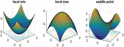
To achieve the optimal solution, the original design should take a specific direction. Linear models generate surfaces that are used to indicate that direction (Bezerra et al., 2008). The dimensions of the critical point can be computed by the first value of the derivative of the function (Bezerra et al., 2008): The first step involves calculating the first derivative and identifying all the zeros within the experimental region, then the possibility of the existence of a saddle point is explored through the calculation of the second derivative (Witek-Krowiak et al., 2014). If the two derivatives are equal to null, a graphical representation of the model will be used to determine the local extreme (Witek-Krowiak et al., 2014). The previous procedure is valid only for single response optimisation. However, the optimal region can be found by visual inspection of the surfaces while the visualisation of the predicted model equation can be obtained by plotting the response surface (contour and 3-D plot; Bezerra et al., 2008). The critical points of the second-order models can be defined as maximum, minimum, or saddle (Figure 7).

Figure 7. Different critical points on a response surface plot (Jin et al., 2017, July).

7.1. Process Parameters for anaerobic digestion

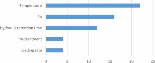
Although the volume and the quality of biogas mainly depend on the nature of the feedstock (Dobre et al., 2014; Qiao et al., 2011), other environmental factors also influence biogas production. These factors include: comminution, dry matter content, digestibility, stirring, and acidification pH, C/N ratio, digester temperature, retention time (hydraulic retention time; HRT and solids retention time; SRT), pressure in the digester, pH of the reactor (which depends on the temperature), organic loading rate (OLR), the volatile fatty acid (VFA) content … (Dobre et al., 2014; Rahim & Ahmed, 2015; Sukor, 2017). Thirty seven (37) parameters were identified in the articles reviewed (Appendix 2), but only the five (5) must occurring (Figure 8) of these parameters were considered and discussed in the current study.

Figure 8. Five active process parameters subjected to variations in articles of interest.

7.1.1. Digestion Temperature

Temperature is a very significant factor in methane formation as bacteria are highly responsive to temperature changes. A wide range of temperatures is possible, generally between 3°C and 70°C (Hoerz et al., 1999). Three temperature ranges are generally distinguished: the psychrophilic temperature range (10–20°C), the mesophilic temperature range (20–40°C), and the thermophilic temperature range (40–70°C). The selection of a temperature range is made after considering the nature of inoculums to be used (Sukor, 2017). The temperature affects the efficiency of the system, methane production, and fermentation (Rajati et al., 2014). Table 1 presents optimum temperatures obtain in reviewed papers. Based on the results in Table 4, it could be pointed that the optimum temperature for biogas production lies in the mesophilic temperature range with some extend to the thermophilic range (35–45°C). The temperature, however, depends on the type of feedstock and has a great effect on the Carbon-to-Nitrogen ratio: temperature affects the depletion of carbon and nitrogen that could cause an inhibitory effect on the anaerobic digestion.

7.1.2. pH

pH is one of the major parameters regulating anaerobic (Vijin Prabhu et al., 2021). The pH of the substrate is determinant of the quantity of methane produced. Based on the reviewed literature, as shown in Table 5, the optimal pH lies in between the acidic and the neutral range (pH 5–7). However, according to (Ozmen & Aslanzadeh, 2009), the pH of a substrate decreases during the fermentation process and increases after the fermentation process. It is thus concluded that for optimum anaerobic digestion and biogas production, the suitable pH should range between 5 and 7. A higher or lower pH could be detrimental to the whole process. An acid solution (hydrochloric acid (HCl), nitric acid (HNO3), sulfuric acid (H2SO4), or acetic acid (CH3COOH)) could be added to the substrate to increase the pH level while a basic solution (sodium hydroxide (NaOH), potassium hydroxide (KOH), ammonia (NH3), or ammonium hydroxide (NH4OH)) is added to decrease the pH level. However, the quantity of solution needed to increase or decrease the pH depends on the initial pH of the substrate. Co-digestion is also a good alternative to regulate the pH of substrates.

7.1.3. Hydraulic retention time

Hydraulic retention time refers to the theoretical duration for which a particle or volume of liquid added to a digester remains there (Nijaguna, 2006). It can be simplified as the length of time the volatile solid remains in the reactor (Dobre et al., 2014). It has a mathematical formula as:

(Equation\,5) $HRT=\frac{V_r}{V_s}\hspace{0.17em}(Days)$(Equation\,5)

Where V_r is the digester volume in m³ and V_s is the quantity of overlay loaded per unit of time in m³/t (Dobre et al., 2014). The hydraulic retention time has a significant effect on the digester’s performance (Ezekoye et al., 2011) and depends on two factors: the process temperature and the substrate type. Table 6 gives a summary of studied substrates and their obtained hydraulic retention times. From the reviewed articles, it is a clear difference between the hydraulic retention time of solid and liquid feedstock has been observed. The optimal hydraulic retention for liquid feedstock is shorter (hours) compared to that of solid feedstock (days). It is thus concluded that the optimal hydraulic retention time for liquid feedstock ranges between 15 and 46 hours while that of solid feedstock lasts between 30 and 40 days.

7.1.4. Pre-treatment

The presence of lignocellulose matter in the feedstock slows down the digestion process. That is why it is recommended to pre-treat substrate before anaerobic digestion (Bala & Mondal, 2019). Pretreatment is meant to break down complex matters into smaller and simpler substance (Bala & Mondal, 2019), thus increases the surface area and surface porosity of the substrate for an increased accessibility for microorganisms and therefore boost biogas production (Memon & Memon, 2020). Pretreated raw materials require lesser processing time than non-pretreated ones (Aziz et al., 2019). There are varieties of pretreatment techniques, which are categorized in groups; these are physical, chemical, thermal, mechanical, and biological pretreatment processes (Bala & Mondal, 2019). Some studies combine two or more pretreatment techniques (Murugan & Sivasamy, 2016; Olatunji et al., 2022). From the reviewed articles (Table 7), it was observed that there is no specific optimum pretreatment type or conditions for all raw materials (the optimum pretreatment condition of wheat straw is very different for that of cow dung). The pretreatment type and conditions depend on the type of raw materials

7.1.5. Organic loading/loading rate

The loading rate is the ratio at which organic matter is supplied to the digester (Jorgensen, 2009). It can also be defined as the number of feedstock introduced per unit volume of the digester capacity per day (Ozmen & Aslanzadeh, 2009). Overfeeding or underfeeding a digester can cause low biogas and methane production; this is why it is important to optimize the loading rate. The optimum loading rate is different for each type of feedstock. Table 8 summarizes a list of selected optimum loading rates.

Table 8. Examples of optimum loading rate

Substrate	Optimum Loading rate	Optimum Response	Reference
SWW	3.5 kg.m^−3.d^−1	5,800 mL/d biogas production 80.8% COD removal	(Chollom et al., 2019)
Palm oil mill effluent (pome)	15.6 g COD/L.d^−1	0.31 LCH4g-1 CODremoved methane yield 67.5% purity of methane	(Chan et al., 2015)
co-digestion of cabbage, cauliflower, and restaurant food waste	0.06 kg ofVS/m3 h for the CCF and FWmixture	High biodegradability (98%), a methane yield of475 mLSTP CH4/g VS	(Beniche et al., 2021)

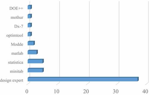
7.2. Some experimental design software

A wild range of statistical software are used today to perform the design of experiment (DOE) as shown in Figure 9. This paper discusses five (5) of these: Design Expert, Minitab, Statistica, Matlab, and Statgraphics Plus.

Figure 9. Statistical software used in the reviewed articles.

7.3. Design expert

The most widely used software (102 out of 200 papers used Design Expert) is a Stat-ease Inc. software package designed to conduct DOE. It supports a wide range of experiments (comparison testing, screening characterization, optimizing, designing robust parameters, and combining and mixing designs) in a user-friendly interface (Khattree & Rao, 2003b) and offers test models that allow the testing of as many as fifty (50) factors. An ANOVA is used to establish the importance of these factors. The impact of these factors on the outcomes is identified with the help of graphical tools.

The Design expert offers eleven (11) graphs that analyze the output of the residuals. The main interactive effects between factors as well as the effects of each of them can be determined by the software. The optimum operating parameters of processes can also be calculated with the help of an optimization feature (Purusottam, 2019). Unlike most software of the same kind, Design Expert provides response transformations for particular cases. The package costs less than $1000 for a single copy.

7.4. Minitab

Minitab is one of the oldest statistical software. It traces its origin from the mid-80s. This software package developed by Barbara F. Ryan can summarize data, produce graphs, and conduct regression analysis, analysis of variance, control charting. It can support basic factorial designs, fractional factorial designs, response surface designs, and Plackett–Burman designs. The response surface support includes Box-Behnken and all forms of central composite designs. However, Minitab does not support sequential experimentation data or data dealing with constrained process spaces.

It is very easy to convert a factorial design to a response surface design. The software also supports interaction graphs involving qualitative factors (very helpful when reading results from such analyses). Minitab has a very convenient optimization section which is easy to use and allows the user to specify the objectives for each response. The results are represented in tabular form and functions which are easy to interpret. The software also supports results overlay. It allows the user to define the axes as well as the optimum values for input parameters. Minitab also supports foldover designs (resolution III to resolution IV; Khattree & Rao, 2003b). The minimum cost for a single-user commercial license for Minitab is $1200 with no annual renewal fee.

7.5. Statistica

It is one of the most powerful and expensive suites of analytical software packages with costs exceeding $2000 and an annual renewal fee for complete modules. The software which was created by StatSoft company and purchased by Dell in 2014 provides a procedure for data analysis, data management, statistics, data mining, machine learning, text analysis, and data display (Anon, 2012). Even though it offers great capacities for design generations, it requires considerable study and practice for full utilization due to the lack of integration of the algorithm design options.

The software offers good tools and graphics for the determination of the source of lack of fit in statistical models. It has a different way of treating qualitative data as opposed to other software. It is also easy to generate foldover designs with Statistica which provides a “square plot” to visualize the results. Statistica provides understandable support for Box-cox transformations, but considerable manipulations of the spreadsheet are necessary before incorporating these transformations in an analysis (Khattree & Rao, 2003b).

The main Statistica package has simple statistics (t-test, correlation, descriptive statistics) and graphing capabilities (bar charts/histograms, trend charts, mean charts, scatter charts, box plots, probability plots, matrix plots) and other statistical capabilities (canonical, cluster, discriminant, factor, log-linear, non-linear, non-parametric, regression, reliability, survival and time series. There are no experimental design or quality control graphing capabilities; Stein et al., 1997). However, generating some experiments is more intensive with Statistica as compared to other software (Khattree & Rao, 2003b).

7.6. Matlab

The Matrix Laboratory (Matlab), developed by Mathworks, is a programming software in a high-level language designed to perform quick and easy calculations (Okereke & Keates, 2018). It provides an innovative interface for design, experimental exploration, and solutions to problems (Colgren, 2007). All data in Matlab are in a matrix form. There is no limitation to the number of rows and columns; the variables can have any number of columns and rows. These variables are called matrix variables and can be any variable in an actual situation (scalars, vectors, or matrices; Okereke & Keates, 2018). The software can be used in all areas of numerical mathematics, as it offers a large library of mathematical functions covering arrays and tables, 2D and 3D graphs and plots and algebra (Colgren, 2007). Matlab has built-in graphs to visualize data and features that create custom graphs. It is widely used in the fields of science and engineering (physics, chemistry, mathematics, and all engineering fields). It is also used in many other fields such as signal flow and communications, image and video editing, monitoring systems, test and measurement, IT finance, bioscience (Colgren, 2007). With its programming environment, Matlab offers support for improving the quality of coding, its ease of maintenance, and minimized failures. It also has tools for creating applications and can be integrated into external applications and languages such as C, Java, .Net and Microsoft Excel (Colgren, 2007).

7.7. Statgraphics

Statgraphics, developed in the early 1980s by renowned Dr. Neil W. Polhemus to teach advanced statistics, was the first computer-based data analysis software. It is a suite of five data analysis products, namely:

• Statgraphics Centurion 18: It is the latest version of the windows desktop software, capable of running more than procedures comprising data visualization, data analysis, ANOVA, design of experiments, statistical data control. Statgraphics Centurion costs a minimum of $765 a year for a single user license

• Statgraphics Stratus is a browser-based software that runs on PC, Mac, Linux, phones, and tablets for data analysis. The challenge is the need for internet access.

• Statgraphics Sigma Express is the Microsoft Excel add-in for quick access to Six Sigma systems on Microsoft Excel’s interface

• Statgraphics Statbeans is a set of JavaScript beans (these are reusable software components written in Java) that can be integrated into applications or slotted onto web pages

• Statgraphics Net Web Services designs for website programmers so they can easily run Statgraphics services straight from their homepages

Statgraphics has been employed in a variety of studies related to health and nutrition, chemistry, pharmacology, medical devices, automotive, mining, environmental studies, and more. It also has an R interface that allows users to extend the use of the software.

7.8. Multi response surface optimization

There are cases when more than one response is under study. These cases are called multi-response optimisation. One of the most popular and useful techniques for solving multi-response optimization problems is the simultaneous optimization method characterized by the concept of the desirability function (Akçay & Anagün, 2013; A. A. Kumar et al., 2013). The desirability function is defined by the following equations:

(Equation\,6) $D=\prod mi=1d_i\frac{1}{m}$(Equation\,6)

Where $d_i$ represents the desirability of i-th response (Witek-Krowiak et al., 2014).

$\text{Or}D\left(Y\right)=\left(d_1{\left(y_1\right)}^{k_1}\times d_2{\left(y_2\right)}^{k_2}\times \dots \times d_X{\left(y_X\right)}^{k_X}\right)1\sum i{k}_i(\text{Equation}\text{7})$

Where $y_i$ denotes the determined value of response i, $d_i\left(y_i\right)$ is the converted desirability value of the i-th response, and $k_i$ represents the relative importance of response i compared to others (Akçay & Anagün, 2013).

The technique was developed by Derringer and Suich in 1980 and consists of converting each response into a desirability function (A. Kumar et al., 2013). The desirability function ranges from $\hspace{0.17em}0\le d_i\le 1$; when $\hspace{0.17em}{d}_i=0$, it means that the response is in an unacceptable region; thus, its value is unacceptable. However, if $d_i=1$, it signifies that the response is at its maximum (Witek-Krowiak et al., 2014).

8. Conclusion

This paper provides a review of the Response Surface Optimization Technique. It concludes that Response surface methodology is a valuable statistics-based optimization method that has helped in many industries and various research fields, especially in the bio-energy field. A total of 55 articles, published from the year 2000 to the year 2022, have been studied using systematic review method. These articles used RSM to optimize biogas production. The review finds that RSM proves to be an effective statistical tool. It has achieved optimum objectives for biogas production: increased biodegradability, optimum biogas yield and methane production, increased Total Solid and reduced Volatile Solids and an increased COD removal.

The greatest advantage of RSM, from the study, is a reduced number of experimental trials, thus, making it time and cost-effective. For the studied papers, thirteen-seven (37) process parameters have been optimized using RSM, over the last two decades. Five (5) of these parameters run active through them as the key process parameters optimized using RSM. Namely,: Temperature, pH, Retention time, Pre-treatment and Loading rate. The reason for the limited use of other parameters is as a result of their lesser impact on the biogas production process. The study identifies the major challenges associated with the use of RSM in biogas production process optimization as a limited experimental range and the need for the steepest descent technique in transferring the optimal area to supply the combinations of parameters during preliminary approximation of parameters. In order to overcome these challenges, techniques to combine RSM with other optimization methods such as the Taguchi, Kriging or the Artificial Neural Network (ANN) are being developed. Design Expert software has been found to be the most used software because of its low cost of use. However, Statistica offers a better efficiency; great tools and graphics for the determination of the source of lack of fit in statistical models. It also uses diverse approaches in treating qualitative data as opposed to the other software.

Acknowledgements

The authors wish to acknowledge the constructive comments of colleagues Donald Kouman, Khadija Sarquah, and Ismail Kone who helped in the improvement of the manuscript.

Disclosure statement

No potential conflict of interest was reported by the author(s).

Additional information

Funding

The authors received no direct funding for this research.

Notes on contributors

Solal Stephanie Djimtoingar

Solal Stephanie Djimtoingar Stephanie, the main author has a Bachelor’s degree in Mechanical Engineering from the University of Mines and Technology and a Masters degree in Sustainable Energy Management from the University of Energy and Natural Resources, both in Ghana. She is currently pursuing a PhD in Sustainable Energy Engineering and Management at the University of Energy and Natural Resources. She specializes in bio-energy generation and waste management. This paper is the first from her PhD thesis, titled: “Evaluation and Optimization of Biogas Production from Calotropis Procera”, supervised by Prof. Nana Sarfo Derkyi Agyemang and Dr. Francis Atta Kuranchie. Joseph Yankyera Kusi is a PhD candidate in Sustainable Energy Engineering and Management at the University of Energy and Natural Resources. He has a Bachelor degree in Renewable Energy Engineering and a Master degree in Sustainable Energy Management, both from the University of Energy and Natural Resources.

Appendix A

Table A1. ~TC~

Substrate	Production method (aerobic or anaerobic digestion)	Process parameters	Dependent variable	Design Method	The objective of the study	Reference	Software
The organic fraction of municipal solid waste (MSW)	Anaerobic digestion	NaOH dose Temperature Time	Biogas yield Soluble Chemical Oxygen Demand Volatile Fatty Acid Phenolic content	Box-Behnken Design	To carry out effective pre-treatment of urban wastewater by biological and thermochemical means.	(Bala & Mondal, 2019)	Design-Expert
(2) Grass silage	Anaerobic digestion	Beating time Temperature	Biogas yield	Face-centered Composite Design	To investigate the effect of beating treatment on grass silage, and develop mathematical models to predict biogas productivity from grass silage.	(Alfarjani, Aboderheeba, & Benyounis, 2013)	Design-Expert
(3) Poultry dropping and pawpaw peels	Anaerobic digestion	Temperature (^0C): x1, pH Retention time (days) Total solids (g/kg) Volatile solids (g/kg): x5	Biogas yield	Central composite rotatable design	To assess the biogas production potential of Carica papaya peelings in co-digestion with poultry manure.	(Dahunsi, Oranusi, Owolabi, & Efeovbokhan, 2016)	Design-Expert
(4) Excess sludge	Anaerobic digestion	pH Sludge Retention Time (SRT)	Biogas yield	Central Composite Design	To study the impact of different pre-treatment techniques on biogas yield.	(Murugan & Sivasamy, 2016)	Minitab
(5) High-load compost leachate	Anaerobic digestion	Chemical Oxygen Demand (COD) of Affluent Hydraulic Retention Time COD/Nitrogen ratio	Chemical oxygen demand removal Biogas production rate	Central Composite Design	To study the treatability of windrow compost leachate using an ABR reactor and also to investigate the COD removal efficiency and biogas production rate (BPR).	(Elyasi, Amani, & Dastyar, 2015)	Dx-7
(6) Rice straw	Anaerobic digestion	Temperature, pH Substrate concentration Agitation time	Biogas yield	Central Composite Design	To improve the biogas yield of anaerobic digestion of rice straw.	(Sathish & Vivekanandan, 2014)	Design-Expert
(7) Saccharina japonica	Anaerobic digestion	Methanogenic inhibitor concentration Temperature	Volatile fatty acids yield Hydrogen production	Central Composite Design	To optimise the yield of volatile fatty acids from the anaerobic digestion of rice straw.	(Kwonsu Jung, Kim, & Park, 2015)
(8) Azolla pinnata biomass	Anaerobic digestion	Pinnata biomass loading Substrate Temperature	Biogas production Chemical Oxygen Demand reduction	Central Composite Design	To investigate anaerobic digestion of Azolla pinnata biomass to improve biogas production.	(V. Kumar, Kumar, Kumar, & Singh, 2020)	Design-Expert
(9) Waste activated sludge	Anaerobic digestion	Quantity of H2O2 Molar proportion of H2O2/Fe^2+ Exposure time	Decay and dehydration of waste activated sludge Elimination of Mixed liquor volatile suspended solids Reduction of capillary suction time Chemical Oxygen Demand and exposure Time Reduction	Central Composite Design	To determine the effects of the quantity of H2O2, H2O2/Fe^2+ molar ratio, and exposure time on the decay and dehydration of wastewater.	(Heng, Isa, Lim, & Ho, 2017)	Design-Expert
(10) Wheat straw	Anaerobic digestion	NH3 Concentration Duration of gas Solid-to-liquid ratio	Methane Yield	Central Composite Design	To optimise the pre-treatment of wheat straw by soaking it in aqueous ammonia to improve the methane yield.	(Lymperatou, Gavala, & Skiadas, 2019)	Design-Expert
(11) Food waste	Anaerobic digestion	Pre-treatment techniques like: Alkaline Ultrasonication Thermal	Food waste solubility Biogas Yield	Face-centered Composite Design	To improve the solubilisation of food waste for methane production.	(Menon, Ren, & Apostolos, 2015)	Minitab
(12) Raw vegetable wastes	Anaerobic digestion	WaP (Waste Plastic) Height to diameter (H/D) Ratio Water Content (WAC) Digestion Time (DT)	Biogas Yield	Central composite rotatable design	To evaluate some process parameters for efficient biogas production from raw plant waste and plastic waste.	(Mukhopadhyay, Sarkar, & Dutta, 2013)	Design-Expert
(13) Rice straw	Anaerobic digestion	Temperature Substrate concentration pH variables	Volatile fatty acids production	Box-Behnken Design	To optimise the yield of volatile fatty acids from the anaerobic digestion of rice straw.	(Kwonsu Jung Et Al., 2015)	Mothur
(14) Waste food materials	Anaerobic digestion	pH Temperature Solid-to-Water Ratio	Biogas production	Box-Behnken Design	To try to digest food waste and produce biogas using a new technique that does not directly involve bacteria	(Pati, Saroha, Behera, Mohapatra, & Mahanand, 2019)	Design-Expert
(15) Petroleum refinery effluent	Anaerobic digestion	Influent chemical oxygen demand Hydraulic Retention Time Up-flow velocity	Chemical Oxygen Demand Removal Biogas Production	Central Composite Design	To further investigate the phenomenon of oil refinery effluent removal in a UASB bioreactor.	(Rastega, Mousavi, Shojaosadati, & Sheibani, 2011)	Design-Expert
(16) Sewage sludge	Anaerobic digestion	Temperature Proportion of NaOH Time	Biogas Yield	Box-Behnken Design	To optimise the heat and alkali decomposition of sewage sludge for a better biogas yield	(Shehu Et Al., 2012)	Matlab
(17) Bagasse based pulp and paper industry wastewater	Anaerobic digestion	Chemical oxygen demand of influent hydraulic retention Time Temperature	Percentage of Chemical Oxygen Demand Removal Chemical Oxygen Demand Removal Rate Biogas Yield	Box-Behnken Design	To study the anaerobic degradation of bagasse effluent from the pulp and paper industry	(Taylor, Sridhar, Sivakumar, & Thirugnanasambandham, N.D.)	Design-Expert
(18) Asparagus stover	Anaerobic digestion	Pre-treatment time NaOH concentration Water dose	Biogas Production	Central Composite Design	To study the interactions between the factors and optimise the sodium hydroxide pre-treatment conditions when the asparagus cane sample is used as feedstock to increase the biogas yield.	(Sun, Liu, Cao, Li, & Wu, 2017)	Design-Expert
(19) Rice mill effluent	Anaerobic digestion	Temperature Alkalinity dose Flow rate	Chemical Oxygen Demand (COD) Removal Biogas Production	Box-Behnken Design	To study the efficiency of seed sludge for biogas generation from rice mill effluent using an anaerobic sludge up-flow bioreactor.	(Karichappan Thirugnanasambandham & Sivakumar, 2014)	Design-Expert
(20) Wastewater sludge	Anaerobic digestion	pH Temperature Incubation time	Dry Cell Weight		To effectively disrupt the flocs with an anionic surfactant, to improve the efficiency of the pre-treatment by using immobilised bacterial cells.	(Ushani, Kavitha, Johnson, Yeom, & Banu, 2016)	Design-Expert
(21) Palm oil mill effluent	Anaerobic digestion	Feed flow rate Up-flow Velocity	Total chemical oxygen demand (TCOD) removal, soluble chemical oxygen demand (SCOD) food-to sludge Solid Retention Time (SRT)	Face-centered Composite Design	To investigate the performance of a reactor in anaerobic digestion of pre-treated palm oil mill effluent.	(Zinatizadeh Et Al., 2006)	Design-Expert
(22) Secondary Tannery sludge (stns)	Anaerobic digestion	Temperature Initial pH	Biogas yield Total methane yield Reduction of volatile solids Decrease of total solids Reduction of Chemical Oxygen Demand		To improve the operating temperature of the reactor and the pH by using adapted inoculum in an attempt to reduce the expected inhibition of NH3, H2S and/or metals	(Mpofu & Oyekola, 2019)	Design-Expert
(23) Food waste and manure	Anaerobic dry co-digestion	Mixture ratio Particle size	Methane yield	Central Composite Design	To optimize the anaerobic dry co-digestion of food waste and manure.	(Cho Et Al., 2013)	Design-Expert
(24) Volatile fatty acids	Anaerobic syntrophic degradation	Propionate, butyrate, acetate, m/a Hydraulic retention time (HRT)	Volatile Fatty Acid removal Biogas Production Rate	Central Composite Design	To optimise methoxy polyp size, entrapment efficiency and percentage drug loading.	(Amani, Nosrati, & Mousavi, 2012)	Design-Expert
(25) Canola residues and cattle dung	Co digestion	Temperature Mixing time Inoculum percentage and Total Solid	Methane production	Box-Behnken Design	To optimise biogas production from canola residues and cattle manure.	(Safari, Abdi, Adl, & Kafashan, 2017)	Design-Expert
(26) Cow dung and coffee pulp	Co digestion	Coffee Pulp Cow Dung Incubation time Temperature	Biogas yield	Box-Behnken Design	To investigate the biogas generation potential of coffee pulp (CP) and cow dung (CD).	(Selvankumar & Govindaraju, 2017)	Design-Expert
(27) Liquid swine manure and sugar beet molasses	Co-fermentation	pH Hydraulic Retention Time Total Solids Content	Biogas Production Rate (BPR) Hydrogen Content (HC) Hydrogen Production Rate (HPR) Hydrogen yield (HY)	Central Composite Design	To study and optimise the operational conditions for the production of hydrogen from sugar beet molasses, co-fermented with pig manure.	(Wu, Lin, & Zhu, 2013)	Design-Expert
(28) Slaughterhouse Wastewater (SWW)	Combine Anaerobic-Aerobic Process	The flow rates The pH The influent Total Organic Carbon concentration	Overall water treatment efficiency (Total Organic Carbon and Total Nitrogen removal and minimized Total Suspended Solid) Biogas yield	Box-Behnken Design	To investigate the effects of influent pH, flow rate and TOC concentration, and their interactive effects on the efficiency of combined anaerobic-aerobic processes on biogas yield for slaughterhouse wastewater treatment	(Bustillo-Lecompte & Mehrvar, 2016)	Design-Expert
(29) Palm Oil Mill Effluent (POME)	Combine Anaerobic-Aerobic Process	Mixed Liquor Volatile Suspended Solids concentration in Anaerobic compartments Organic loading rates in Anaerobic Compartment	Reduction of organic matter (chemical oxygen demand (COD), biochemical oxygen demand (BOD) and total suspended solids (TSS) concentrations)	Central composite rotatable design (CCRD)	To design and monitor the anaerobic and aerobic thermophilic treatment of palm oil mill effluent in the integrated anaerobic-aerobic bioreactor with regards to the simultaneous effects of the three process parameters.	(Chan, Chong, & Law, 2014)	Design-Expert
(30) Digested and undigested poultry litter	Fermentation	Undigested poultry litter Concentration Yeast Extract Concentration pH	Single-cell protein production	Central Composite Design	To use undigested poultry litter (UPL) as a substrate for the generation of single-cell protein (SCP) through the use of a yeast extract.	(Jalasutram & Kataram, 2013)	Doe++
(31) Cold active β-galactosidase	Fermentation	pH whey tryptone	Cold active β-galactosidase production	Central Composite Design	To screen for the most relevant influencing factors affecting the production of cold-active β-galactosidase by a culture of Enterobacter ludwigii (MCC 3423) batches and to optimise further the levels of the relevant variables screened.	(Alikunju Et Al., 2017)	Design-Expert
(32) Spent tea leaves	Fermentation	Temperature, pre-treatment time Solid-to-liquid Ratio Dilute acid or alkaline ratio	Dilute acid and alkaline pre-treatment conditions of Spent tea leaves	Box-Behnken Design	To optimise the conditions for dilute acid and alkaline pre-treatment of spent tea leaves.	(Germec, Bader, & Turhan, 2018)	Design-Expert
(33) Acid pre-treated Food waste hydrolysate	Fermentation	Time of fermentation Immobilized bead ratio	Ethanol yield	Central Composite Design	To study ethanol production from acid-pre-treated food waste hydrolysate using Saccharomyces cerevisiae 74D694 immobilised under different conditions in a batch experiment.	(Paulraj & Debraj, 2017)	Statistica
(34) Laminaria japonica	Fermentation	Hydrochloric acid (HCL) Concentrations Heating temperatures Reaction times	Hydrogen production	Box-Behnken Design	To improve the production of fermentative hydrogen peroxide (FHP) from Laminaria japonica using combined pre-treatment techniques (acid þ thermal).	(Kyung-Won Jung, Kim, Kim, & Shin, 2011)	Design-Expert
(35) De-oiled jatropha	Fermentation	Substrate concentrations Temperatures pH	Biohydrogen production	Central Composite Design	To optimise the hydrogen fermentation process from de-oiled Jatropha waste	(G. Kumar, Sivagurunathan, Peter, & Lin, 2014)	Statistica
(36) Rhodobacter sphaeroides kku-ps5 (bio-hydrogen)	Fermentation	Initial pH Light Intensity Mo Concentration	Lab/PNSH bacterial ratio Initial Cell Concentration	Central Composite Design	To perform the bio-augmentation of Rhodobacter sphaeroides KKU-PS5 with Lactobacillus delbrueckii ssp to produce hydrogen.	(Laocharoen, Reungsang, & Plangklang, 2015)	Design-Expert
(37) Fresh compost leachate	Fermentation	Leachate volume Glucose concentration	Bio-Hydrogen Production	D-Optimal Design.	To study the applicability of bio-hydrogen generation using fresh compost leachate as a nutrient source.	(Liu Et Al., 2011)	Design-Expert
(38) Sugar cane molasses	Fermentation	Fermentation time pH Initial Total Reducing Sugar (TRS) Temperature Concentration in Sugar Cane Molasses	Ethanol Yield	Box-Behnken Design	To optimise the process parameters of ethanol production from sugarcane molasses by Zymomonas.	(Maiti, Rathore, & Srivastava, 2011)	Minitab
(39) Cyperus difformis	Fermentation	Solid/Liquid Ratio Concentration of NaOH Proportion of H2O2 Duration (H)	Sugar Yield	Box-Behnken Design	To examine the potential of yellow nutsedge for bioethanol generation.	(Ramaraj & Unpaprom, 2019)	Design-Expert
(40) Potato waste	Fermentation	Potato Waste Concentration pH Temperature Fermentation time	Biohydrogen production	Central Composite Design	To optimise biohydrogen production from potato waste	(Sekoai, Ayeni, & Daramola, 2017)	Statistica
(41) Mutant strain zjuel31410 of bacillus licheniformis	Fermentation	Temperature Fermentation time Shaking speed Inoculating volume Seed age Medium Volume	Elastase production Cell growth	Central Composite Design	To optimise the culture conditions of Bacillus licheniformis ZJUEL31410, and to analyse the effect of growth factors and elastin on elastase production and cell growth.	(Qi-He, Hui, Hai-Feng, Hui, & Guo-Qing, 2007)	Statistical Analysis Software
(42) Marine bacterium	Fermentation	F. Bombycis Soluble starch (NH4)2SO4	Macrolide Compound Production	Box-Behnken Design	To improve the production of a 24-membered ring macrolide compound.	(H. Chen Et Al., 2013)	Minitab
(43) succinogenes strain BE-1	fermentation	Glucose Yeast extract Magnesium carbonate	Succinic acid production	Central Composite Design	To investigate the optimisation of succinic acid fermentation with A. succino-genes strain BE-1	(Zhang, Li, Zhang, Wang, & Xing, 2012)	Design-Expert
(44) Cordyceps Militaris	Fermentation	Concentration of sucrose peptone MgSO4·7H2O	Yield of Endo-Polysaccharide	Box-Behnken Design	To optimise the fermentation environment that influenced the endo-polysaccharide yield of cultured Cordyceps militaris N102 mycelia.	(Liang, Zhang, Zhang, Zhang, & Lü, 2012)	Statistical Analysis Software
(45) Palm oil mill effluent (POME)	Fermentation (anaerobic)	The pH Temperature Chemical Oxygen Demand (COD)	Hydrogen production Hydrogen production rate	Central Composite Design	To determine the optimal conditions for hydrogen production and the maximum rate of hydrogen production from palm oil mill effluent.	(Cheong Et Al., 2022)
(46) Sugar Beet Pulp	Hydrolysis	The size of particles The enzyme proportions The time required to convert the Sugar Beet pulp pectin to Pectic Oligosaccharides	Enzymatic Pectic Oligosaccharides (POS) yield	Central Composite Design	To study the yield of POS (Enzymatic Pectic Oligosaccharides) from sugar beet pulp (SBP) depending on parameters such as enzyme concentration, particle size and conversion time.	(Babbar, Dejonghe, Sforza, & Elst, 2017)	Design-Expert
(47) Bacillus sp. Rky3	Hydrolysis	Corn Starch Yeast Extract Corn steep liquor Inoculum Size	Production of alkaline protease	Central Composite Design	To identify and optimize the significant variables for alkaline protease production using Bacillus sp. RKY3.	(Reddy, Wee, Yun, & Ryu, 2008)	Design-Expert
(48) Food Waste with Sewage Sludge	Anaerobic digestion	Hydraulic Retention time Sludge recycle ratio Water to feed ratio Sewage sludge to food waste ratio	Methane flow Chemical Oxygen Demand (COD) Volatile solids	Box-Behnken Design	To develop the simulation model to determine the feasibility of the biogas generation from the ACD of FW with SS and examining the effect of HRT, water to feed ratio (kg/kg), sludge recycle ratio and SS to FW ratio (kg/kg) on the methane flow, chemical oxygen demand (COD) and volatile solids (VS) removal efficiencies	(Abdul Aziz et al., 2019)	Design Expert v13
(49) Okra waste and pig manure	anaerobic co-digestion	Codigestion ratio Percentage of polypyrrole magnetite nanocomposites (Ppy/Fe3O4) Percentage of antagonists (humic acid and arsenic acid)	Biomethane yield P release	Central Composite Design	To analyze the influence of variables such as co- digestion, iron nanocomposite (PPy/Fe3O4), humic acid and arsenic oxide on biomethane yield and phos- phorus release from okra waste and pig manure	(Ugwu & Enweremadu, 2022)	Design Expert
(50) Green algae	Anaerobic digestion	Temperature Initial pH Nickel nanoparticles concentration	Biogas yield	Central Composite Design	To optimize nickel nanoparticles concentration for an optimum biogas yield	(Zaidi et al., 2019)	Design Expert
(51) Corn chaff and cow dung	Anaerobic co-digestion	Mixture ratio Hydraulic retention time	Biogas yield	Central Composite Design	To optimize biogas production from biomass wastes through anaerobic digestion using CCD of RSM, and python coding	(Iweka et al., 2021)
(52) Dairy industry effluent	Anaerobic digestion	Sludge percentage Temperature	Biogas yield Volatile solid removal		To study the interaction effect of sludge percentage and temperature at the level of one percent on the volumetric indices of biogas production	(Nouri et al., 2020)
(53) Prosopis juliflora seeds, water hyacinth, dry leaves, and cow manure	Anaerobic Co-digestion	pH Temperature	Methane yield Biodegradability TS reduction	Central Composite Design	To produce the biogas by anaerobic degradation of Prosopis juliflora pods, water hyacinth, dry leaves	(Vijin Prabhu et al., 2021)	Design Expert
(54) Flower waste	Anaerobic digestion	pH Temperature Substrate concentration Agitation time	Biogas yield		To augment the biogas production from flower waste through optimization and pretreatment techniques	(Gopal et al., 2021)

References

- Abdeshahian, P., Shiun, J., Shin, W., Hashim, H., & Lee, C. T. (2016). Potential of biogas production from farm animal waste in Malaysia. Renewable and Sustainable Energy Reviews, 60, 714–35. https://doi.org/10.1016/j.rser.2016.01.117
- Ait-Amir, B., Pougnet, P., & El Hami, A. (2015). Meta-model development. In A. El Hami & P. Pougnet (Eds.), Embedded Mechatronic Systems, 2, 151–179. Elsevier. https://doi.org/10.1016/b978-1-78548-014-0.50006-2
- Akçay, H., & Anagün, A. S. (2013). Multi response optimization application on a manufacturing Factory. Mathematical and Computational Applications, 18(3), 531–538. https://doi.org/10.3390/mca18030531
- Akpoti, K., Kabo-bah, A. T., & Zwart, S. J. (2019). Agricultural land suitability analysis: State-of-the-art and outlooks for integration of climate change analysis. Agricultural Systems, 173(February), 172–208. https://doi.org/10.1016/j.agsy.2019.02.013
- Alfarjani, F., Aboderheeba, A. K. M., & Benyounis, K. (2013). Modelling anaerobic digestion process for grass silage after beating treatment using design of experiment. In I. Dincer, C. O. Colpan, & F. Kadioglu (Eds.), Causes, Impacts and Solutions to Global Warming (pp. 675–695). Springer Science & Business Media. https://doi.org/10.1007/978-1-4614-7588-0
- Alikunju, A. P., Joy, S., Rahiman, M., Rosmine, E., Antony, A. C., Solomon, S., Saramma, K. M. A. V., & Mohamed, K. P. K. A. A. (2017). A statistical approach to optimize cold active β-galactosidase production by an arctic sediment pscychrotrophic bacteria, enterobacter ludwigii (MCC 3423) in cheese whey. Catalysis Letters. https://doi.org/10.1007/s10562-017-2257-4
- Amani, T., Nosrati, M., & Mousavi, S. M. (2012). Response surface methodology analysis of anaerobic syntrophic degradation of volatile fatty acids in an upflow anaerobic sludge bed reactor inoculated with enriched cultures. Biotechnology and Bioprocess Engineering, 17(1), 133–144. https://doi.org/10.1007/s12257-011-0248-7
- Anon. (2012). Statsoft Statistica: a guide - Statistics Views. Statsoft Company. https://www.statisticsviews.com/details/tools/13a69fb94dc/Statsoft-Statistica-a-guide.html
- Anunputtikul, W., & Rodtong, S. (2004). Laboratory scale experiments for biogas production from cassava tubers. School of Biology, Institute of Science, Suranaree University of Technology. http://sutir.sut.ac.th:8080/jspui/handle/123456789/1001
- Atkinson, A. C., & Fedorov, V. V. (1975). Optimal design : Experiments for discriminating between several models. Biometrika, 62(2), 289–303. https://doi.org/10.1093/biomet/62.2.289
- Aydar, A. Y. (2018). Utilization of response surface methodology in optimization of extraction of plant materials. Statistical Approaches with Emphasis on Design of Experiments Applied to Chemical Processes, 157–169. https://doi.org/10.5772/65616
- Aziz, M. A., Anuar, K., Elsergany, M., Anuar, S., Jorat, M. E., Yaacob, H., Ahsan, A., & Imteaz, M. A. (2019). Recent advances on palm oil mill effluent (POME) pretreatment and anaerobic reactor for sustainable biogas production. Renewable and Sustainable Energy Reviews, February, 109603. https://doi.org/10.1016/j.rser.2019.109603
- Bala, R., & Mondal, M. K. (2019). Study of biological and thermo-chemical pretreatment of organic fraction of municipal solid waste for enhanced biogas yield. Environmental Science and Pollution Research, 27(22), 27293–27304. https://doi.org/10.1007/s11356-019-05695-w
- Bartz-Beieslstein, T., Chiarandini, M., Paquete, L., & Preuss, M. (Ed.). (2010). Experimental methods for the analysis of optimization algorithms (pp. 311–336). Berlin: Springer.
- Bas, D., & Boyaci, I. H. (2007). Modeling and optimization i: Usability of response surface methodology. Journal of Food Engineering, 78(3), 836–845. https://doi.org/10.1016/j.jfoodeng.2005.11.024
- Bashir, M. J. K., Amr, S. S. A., Aziz, S. Q., Aun, N. C., Sethupathi, S., Technology, G., Tunku, U., & Rahman, A. (2015). Wastewater treatment processes optimization using response surface methodology (RSM) compared with conventional methods. Review and Comparative Study Department of Environmental Engineering, Faculty of Engineering School of Civil Engineering, Enginee. Middle-East Journal of Scientific Research, 23(2), 244–252. https://doi.org/10.5829/idosi.mejsr.2015.23.02.52
- Beevi, B. S., Jose, P. P., & Madhu, G. (2014). Optimization of process parameters affecting biogas production from organic fraction of municipal solid waste via anaerobic digestion. International Journal of Bioengineering and Life Sciences, 8(1), 43–48. waset.org/Publication/9997252
- Beniche, I., Hungría, J., El Bari, H., Siles, J. A., Chica, A. F., & Martín, M. A. (2021). Effects of C/N ratio on anaerobic co-digestion of cabbage, cauliflower, and restaurant food waste. Biomass Conversion and Biorefinery, 11(5), 2133–2145. https://doi.org/10.1007/s13399-020-00733-x
- Bessou, C., Ferchaud, F., Gabrielle, B., & Mary, B. (2011). Biofuels, greenhouse gases and climate change. Sustainable Agriculture Volume, 2, 365–468. https://doi.org/10.1051/agro
- Bezerra, M. A., Santelli, R. E., Oliveira, E. P., Villar, L. S., & Escaleira, L. A. (2008). Response surface methodology (RSM) as a tool for optimization in analytical chemistry. Talanta, 76(5), 965–977. https://doi.org/10.1016/j.talanta.2008.05.019
- Box, G. E. P., & Wilson, K. B. (1951). On the statistical attainment of optimum conditions. Journal of the Royal Statistical Society Series B, 13, 1–45. https://doi.org/10.1111/j.2517-6161.1951.tb00067.x
- Boyaci, I. H. (2005). A new approach for determination of enzyme kinetic constants using response surface methodology. Biochemical Engineering Journal, 25(1), 55–62. https://doi.org/10.1016/j.bej.2005.04.001
- Bradley, N. (2009). Response surface methodology. Comprehensive Chemometrics, 1, 345–390. https://doi.org/10.1016/B978-044452701-1.00083-1
- Breig, S. J. M., & Luti, K. J. K. (2021). Response surface methodology: A review on its applications and challenges in microbial cultures. Materials Today: Proceedings, 42, 2277–2284. https://doi.org/10.1016/J.MATPR.2020.12.316
- Buaisha, M., Balku, S., & Özalp-Yaman, Ş. (2020). Heavy metal removal investigation in conventional activated sludge systems. Civil Engineering Journal (Iran), 6(3), 470–477. https://doi.org/10.28991/cej-2020-03091484
- Bustillo-lecompte, C. F., & Mehrvar, M. (2017). Treatment of actual slaughterhouse wastewater by combined anaerobic–aerobic processes for biogas generation and removal of organics and nutrients: An optimization study towards a cleaner production in the meat processing industry. Journal of Cleaner Production, 141, 278–289. https://doi.org/10.1016/j.jclepro.2016.09.060
- Central Composite Designs (CCD). (2013). In NIST/SEMATECH e-Handbook of Statistical Methods. https://www.itl.nist.gov/div898/handbook/pri/section3/pri3361.htm
- Chan, Y., Chong, M., & Law, C. (2015). Optimization of thermophilic anaerobic-aerobic treatment system for Palm Oil Mill Effluent (POME). Frontiers of Environmental Science & Engineering, 9(2), 334–351. https://doi.org/10.1007/s11783-014-0626-4
- Chelladurai, S. J. S., Murugan, K., Ray, A. P., Upadhyaya, M., Narasimharaj, V., & Gnanasekaran, S. (2020). Optimization of process parameters using response surface methodology: A review. Materials Today: Proceedings, 37(Part 2), 1301–1304. https://doi.org/10.1016/j.matpr.2020.06.466
- Cheong, W. L., Jing Chan, Y., Joyce Tiong, T., Chan Chong, W., Kiatkittipong, W., Kiatkittipong, K., Mohamad, M., Hanita Daud, I. W. K. S., Mutiara Sari, M., & Wei Lim, J. (2022). Anaerobic Co-Digestion of Food Waste with Sewage Sludge. Simulation and Optimization for Maximum Biogas Production” Water, 14(7), 1075. https://doi.org/10.3390/w14071075
- Chinneck, J. W. (2007). Feasibility and Infeasibility in Optimization:: Algorithms and Computational Methods (Vol. 118). Springer Science & Business Media.
- Chollom, M. N., Rathilal, S., Swalaha, F. M., Bakare, B. F., & Tetteh, E. K. (2019). Comparison of response surface methods for the optimization of an upflow anaerobic sludge blanket for the treatment of slaughterhouse wastewater. Environmental Engineering Research, 25(1), 114–122. https://doi.org/10.4491/eer.2018.366
- Colgren, R. (2007). Introduction to MATLAB. Basic MATLAB®, Simulink®, and Stateflow®, 1–42. American Institute of Aeronautics and Astronautics. https://doi.org/10.2514/5.9781600861628.0001.0042
- Copelli, D., Falchi, A., Ghiselli, M., Lutero, E., Osello, R., Riolo, D., Schiaretti, F., & Leardi, R. (2018). Sequential “asymmetric” D-optimal designs: A practical solution in case of limited resources and not equally expensive experiments. Chemometrics and Intelligent Laboratory Systems, 178, 24–31. https://doi.org/10.1016/J.CHEMOLAB.2018.04.017
- Dahunsi, S. O., Oranusi, S., Owolabi, J. B., & Efeovbokhan, V. E. (2016). Comparative biogas generation from fruit peels of Fluted Pumpkin (Telfairia occidentalis) and its optimization. Bioresource Technology, 221, 517–525. https://doi.org/10.1016/j.biortech.2016.09.065
- De Aguiar, P. F., Bourguignon, B., Khots, M. S., Massart, D. L., Phan-Than-Luu, R., & Leardi, R. (1995). D-optimal designs. Chemometrics and Intelligent Laboratory Systems, 30(2), 199–210. https://doi.org/10.1016/0169-7439(94)00076-X
- Dobre, P., Nicolae, F., & Matei, F. (2014). Main factors affecting biogas production - an overview. Romanian Biotechnological Letters, 19(3), 9283–9296.
- Elyasi, S., Amani, T., & Dastyar, W. (2015). A comprehensive evaluation of parameters affecting treating high-strength compost leachate in anaerobic baffled reactor followed by electrocoagulation-flotation process. Water, Air, and Soil Pollution, 226(4). https://doi.org/10.1007/s11270-014-2279-0
- Enitan-folami, A. M., Adeyemo, J., Swalaha, F. M., & Kumari, S. (2016). Optimization of biogas generation using anaerobic digestion models and computational intelligence approaches. August 2019 https://doi.org/10.1515/revce-2015-0057
- Ezekoye, V., Ezekoye, B., & Offor, P. O. (2011). Effect of retention time on biogas production from poultry droppings and cassava peels. Nigerian Journal of Biotchnology, 22, 53–59. https://doi.org/10.4314/NJB.V22I0
- Gopal, L. C., Govindarajan, M., Kavipriya, M. R., Mahboob, S., Al-Ghanim, K. A., Virik, P., Ahmed, Z., Al-Mulhm, N., Senthilkumaran, V., & Shankar, V. (2021). Optimization strategies for improved biogas production by recycling of waste through response surface methodology and artificial neural network: Sustainable energy perspective research. Journal of King Saud University - Science, 33(1), 101241. https://doi.org/10.1016/j.jksus.2020.101241
- Guthrie, W., Filliben, A., & Tarvainen, T. (2013). NIST/SEMATECH e-handbook of statistical methods. Process Modeling.
- Gyenge, L., Ráduly, B., Crognale, S., Lányi, S., & Ábrahám, B. (2014). Cultivating conditions optimization of the anaerobic digestion of corn ethanol distillery residuals using response surface methodology +. Central European Journal of Chemistry, 12(8), 68–876. https://doi.org/10.2478/s11532-014-0542-2
- Handbook of Statistical Methods. (2013). In NIST/SEMATECH e-Handbook of Statistical Methods. https://www.itl.nist.gov/div898/handbook/pri/section7/pri7.htm#Rotatability
- Heng, G. C., Isa, M. H., Lim, J. W., Ho, Y. C., & Zinatizadeh, A. A. L. (2017). Enhancement of anaerobic digestibility of waste activated sludge using photo-Fenton pretreatment. Environmental Science and Pollution Research, 24(35), 27113–27124. https://doi.org/10.1007/s11356-017-0287-5
- Hoefsloot, H. C. J., Vis, D. J., Westerhuis, J. A., Smilde, A. K., & Jansen, J. J. (2009). 2.23 - Multiset data analysis: ANOVA simultaneous component analysis and related methods. In Steven D. Brown, T. Romá, & W. Beata (Eds.), Comprehensive Chemometrics (Vol. 2, pp. 453–472). Elsevier. https://doi.org/10.1016/B978-044452701-1.00054-5
- Hoerz, T., Krämer, P., Klingler, B., Kellner, C., Wittur, T., Klopotek, F. V., Krieg, A., & Euler, H. (1999). Biogas digest volume II biogas-Application and Product Development Information and Advisory Service on Appropriate Technology. German Agency for Technical Cooperation (GTZ). Eschborn. Germany.
- Hromi, J. D. (1957). Some concepts of experimental design. Corrosion, 13(11), 61–64. https://doi.org/10.5006/0010-9312-13.11.61
- Iversen, G. R., & Norpoth, H. (1987). Analysis of variance (quantitative applications in the social science). SAGE Publications. first
- Iweka, S. C., Owuama, K. C., Chukwuneke, J. L., & Falowo, O. A. (2021). Optimization of biogas yield from anaerobic co-digestion of corn-chaff and cow dung digestate: RSM and python approach. Heliyon, 7(11), e08255. https://doi.org/10.1016/j.heliyon.2021.e08255
- Jin, C., Ge, R., Netrapalli, P., Kakade, S. M., & Jordan, M. I. (2017, July). How to escape saddle points efficiently. In International Conference on Machine Learning (pp. 1724–1732). PMLR.
- Jorgensen, P. J. (2009). Biogas - green energy process. design. energy supply. environment (A. B. Nielsen & F. Bendixen, Eds.). Digisource Danmark A/S.
- Jung, K., Kim, W., Park, G. W., Seo, C., Chang, H. N., & Kim, Y. C. (2015). Optimization of volatile fatty acids and hydrogen production from Saccharina japonica: Acidogenesis and molecular analysis of the resulting microbial communities. Applied Microbiology and Biotechnology, 99(7), 3327–3337.
- Khattree, R., & Rao, C. R. (2003a). Industrial experimentation for screening. Handbook of Statistics, 22. https://www.biblio.com/9780444506146
- Khattree, R., & Rao, C. R. (2003b). Statistics in industry (Vol. 22). Gulf Professional Publishing. https://www.biblio.com/9780444506146
- Kilickap, E. (2010). Modeling and optimization of burr height in drilling of Al-7075 using Taguchi method and response surface methodology. The International Journal of Advanced Manufacturing Technology, 49(9–12), 911–923. https://doi.org/10.1007/s00170-009-2469-x
- Kumar, A., Kumar, V., & Kumar, J. (2013). Multi-response optimization of process parameters based on response surface methodology for pure titanium using WEDM process. The International Journal of Advanced Manufacturing Technology, 68(9–12), 2645–2668. https://doi.org/10.1007/s00170-013-4861-9
- Kumar, G., Sivagurunathan, P., Peter, S. K., & Lin, B. C. (2014). Modeling and optimization of biohydrogen production from de-oiled jatropha using the response surface method. Arabian Journal for Science and Engineering, 40(1), 15–22. https://doi.org/10.1007/s13369-014-1502-z
- Lane, D. M. (2015). Introduction to ANOVA (analysis of variance). In G. Ritzer (Ed.),The Blackwell Encyclopedia of Sociology. https://doi.org/10.1002/9781405165518.wbeosa055.pub2
- Leiviska, K. (2013). Introduction to experiment design. In Handbook of Experimental Methods for Process Improvement (pp. 1–16). Control Engineering Laboratory. https://doi.org/10.1007/978-1-4615-6025-8_1
- Makela, M. (2017). Experimental design and response surface methodology in energy applications: A tutorial review. Energy Conversion and Management, 151(September), 630–640. https://doi.org/10.1016/j.enconman.2017.09.021
- Memon, M. J., & Memon, A. R. (2020). Wheat straw optimization via its efficient pretreatment for improved biogas production. Civil Engineering Journal (Iran), 6(6), 1056–1063. https://doi.org/10.28991/cej-2020-03091528
- Menon, A., Ren, F., Jing-Yuan, W., & Giannis, A. (2016). Effect of pretreatment techniques on food waste solubilization and biogas production during thermophilic batch anaerobic digestion. Journal of Material Cycles and Waste Management, 18(2), 222–230. https://doi.org/10.1007/s10163-015-0395-6
- Mkruqulwa, U., Okudoh, V., & Oyekola, O. (2019). Optimizing methane production from Co ‑ digestion of cassava biomass and winery solid waste using response surface methodology republic of South Africa. Waste and Biomass Valorization, 11(9), 4799–4808. https://doi.org/10.1007/s12649-019-00801-y
- Montgomery, D. C. (2017). Design and analysis of experiments. John Wiley & Sons, Inc. 8th editio. https://doi.org/10.1002/9783527809080.cataz11063
- Mpofu, A. B., & Oyekola, P. J. W. O. O. (2019). Anaerobic digestion of secondary tannery sludge : optimisation of initial pH and temperature and evaluation of kinetics. Waste and Biomass Valorization. https://doi.org/10.1007/s12649-018-00564-y
- Mukumba, P., Makaka, G., & Mamphwell, S. (2016). Anaerobic digestion of donkey dung for biogas production. South African Journal of Science, 112(7–8), 1–4.
- Murugan, P. D. D., & Sivasamy, M. S. A. (2016). Optimization and biokinetic studies on pretreatment of sludge for enhancing biogas production. International Journal of Environmental Science and Technology, 14(4), 813–822. https://doi.org/10.1007/s13762-016-1191-0
- Muthuvelayudham, R. V., Jiang, T, C., Schuster, T., Li, G.-X., Daniel, P. T., & Lü, J. (2006). Fermentative production and kinetics of cellulase protein on Trichoderma reesei using sugarcane bagasse and rice straw. African Journal of Biotechnology, 5(20), 1873–1881. https://doi.org/10.1158/1535-7163.MCT-06-0063
- Nevzorova, T., & Karakaya, E. (2020). Explaining the drivers of technological innovation systems : The case of biogas technologies in mature markets. Journal of Cleaner Production, 259, 120819. https://doi.org/10.1016/j.jclepro.2020.120819
- Nielsen, H. B., Uellendahl, H., & Ahring, B. K. (2007). Regulation and optimization of the biogas process : Propionate as a key parameter. Biomass and bioenergy, 31(11-12), 820–830. https://doi.org/10.1016/j.biombioe.2007.04.004
- Nijaguna, B. (2006). Biogas Technology. New Age International. https://books.google.co.in/books?id=QfLDbf3qbcEC
- Nnaemeka, S., Christopher, U., Enweremadu, C., Nnaemeka Ugwu, S., & Chintua Enweremadu, C. (2022). Environmental technology (Print) (Optimization of iron-enhanced anaerobic digestion of agro-wastes for biomethane production and phosphate release Optimization of iron-enhanced anaerobic digestion of agro-wastes for biomethane production and phosphate release. https://doi.org/10.1080/09593330.2022.2061379
- Nooraziah, A., & Tiagrajah, V. J. (2014). A study on regression model using response surface methodology. Applied Mechanics and Materials, 666(September), 235–239. https://doi.org/10.4028/www.scientific.net/AMM.666.235
- Nor, W., & Wan, N. (2020). Response Surface Methodology (Rsm): Learn and Apply. School of Chemical and Energy Engineering, BMU,17/2/2020. February. https://www.researchgate.net/publication/339301705
- Nouri, N., Asakereh, A., & Soleymani, M. (2020). Investigating the interaction effects of inoculation and temperature on biogas production from dairy industry effluent in anaerobic digestion process. Iranian Journal of Biosystems Engineering, 52(1), 79–93. https://doi.org/10.12691/rse-5-1-5
- Okereke, M., & Keates, S. (2018). A brief introduction to MATLABTM. In Finite Element Applications. Springer Tracts in Mechanical Engineering, 9783319671246, 27–45. Springer, Cham. https://doi.org/10.1007/978-3-319-67125-3_2
- Olatunji, K. O., Ahmed, N. A., Madyira, D. M., Adebayo, A. O., Ogunkunle, O., & Adeleke, O. (2022). Performance evaluation of ANFIS and RSM modeling in predicting biogas and methane yields from Arachis hypogea shells pretreated with size reduction. Renewable Energy, 189, 288–303. https://doi.org/10.1016/j.renene.2022.02.088
- Olawoye, B. (2016). Comprehensive handout on Central Composite Design (CCD). July, 1–47. https://www.researchgate.net/publication/308608329_A_COMPREHENSIVE_HANDOUT_ON_CENTRAL_COMPOSITE_DESIGN_CCD
- Olivero, R. A., Nocerino, J. M., & Deming, S. N. (1998). Experimental design and optimization. In Chemometrics in Environmental Chemistry-Statistical Methods (pp. 73–122). Springer, Berlin, Heidelberg. https://doi.org/10.1007/978-3-540-49148-4-3
- Ozmen, P., & Aslanzadeh, S. (2009). Biogas production from municipal waste mixed with different portions of orange peel. University of Boras.
- Pati, A. R., Saroha, S., Behera, A. P., Mohapatra, S. S., & Mahanand, S. S. (2019). The anaerobic digestion of waste food materials by using cow dung : a new methodology to produce biogas. Journal of the Institution of Engineers (India): Series E, 100(1), 111–120. https://doi.org/10.1007/s40034-019-00134-4
- Penny, W., & Henson, R. (2007). Analysis of variance. Statistical Parametric Mapping: The Analysis of Functional Brain Images, 166–177. https://doi.org/10.1016/B978-012372560-8/50013-9
- Purusottam, M. (2019). Factors affecting Design of Experiment (DOE) and softwares of DOE. https://www.slideshare.net/DauRamChandravanshi1/factors-affecting-design-of-experiment-doe-and-softwares-of-doe/22
- Qiao, W., Yan, X., Ye, J., Sun, Y., Wang, W., & Zhang, Z. (2011). Evaluation of biogas production from different biomass wastes with/without hydrothermal pretreatment. Renewable Energy, 36(12), 3313–3318. https://doi.org/10.1016/j.renene.2011.05.002
- Rahim, O. M. A., & Ahmed, A. I. (2015). Biogas production from poultry manure. August.
- Rajati, H., Ardjmand, M., & Rajati, F. (2014). A review of biogas production methods from wastes and sewage and the process explanation. Archives of Hygiene Sciences, 3(3), 140–151.
- Ramaraj, R., & Unpaprom, Y. (2019). Optimization of pretreatment condition for ethanol production from cyperus difformis by response surface methodology. 3 Biotech, 9(6), 1–9. https://doi.org/10.1007/s13205-019-1754-0
- Ranganath, M. S. (2015). Surface roughness prediction model for CNC turning of EN-8 steel using response surface methodology. International Journal of Emerging Technology and Advanced Engineering, 5(6), 135–143. https://www.researchgate.net/publication/279061190_Surface_Roughness_Prediction_Model_for_CNC_Turning_of_EN-8_Steel_Using_Response_Surface_Methodology
- Rastega, S. O., Mousavi, S. M., Shojaosadati, S. A., & Sheibani, S. (2011). Optimization of petroleum refinery effluent treatment in a UASB reactor using response surface methodology. Journal of Hazardous Materials, 197, 26–32. https://doi.org/10.1016/j.jhazmat.2011.09.052
- Reddy, L. V. A., Wee, Y., Yun, J., & Ryu, H. 2008. Optimization of alkaline protease production by batch culture of Bacillus sp . RKY3 through Plackett – Burman and response surface methodological approaches. Bioresource technology, 99(7): 2242–2249. https://doi.org/10.1016/j.biortech.2007.05.006
- Rockafellar, R. T. (2015). Convex Analysis. Princeton University Press, 1983, 425–432. https://doi.org/10.1515/9781400873173-011
- Sarabia, L. A., & Ortiz, M. C. (2009). Response surface methodology. Comprehensive Chemometrics, 1(May), 345–390. https://doi.org/10.1016/B978-044452701-1.00083-1
- Sathish, S., & Vivekanandan, S. (2014). Optimization of different parameters affecting biogas production from rice straw : An analytical approach. International Journal of Simulation: Systems, Science and Technology,15, 78–84. https://doi.org/10.5013/IJSSST.a.15.02.11
- Sathish, S., & Vivekanandan, S. (2016). Parametric optimization for floating drum anaerobic bio-digester using response surface methodology and artificial neural network. Alexandria Engineering Journal, 55(4), 3297–3307. https://doi.org/10.1016/j.aej.2016.08.010
- Sawyer, S. F. (2009). Analysis of variance: the fundamental concepts. Journal of Manual & Manipulative Therapy, 17(2), 27E–38E. https://doi.org/10.1179/jmt.2009.17.2.27e
- Shen, Y., Linville, J. L., Urgun-demirtas, M., Mintz, M. M., & Snyder, S. W. (2015). An overview of biogas production and utilization at full-scale wastewater treatment plants (WWTPs) in the United States : Challenges and opportunities towards energy-neutral WWTPs. Renewable and Sustainable Energy Reviews, 50, 346–362. https://doi.org/10.1016/j.rser.2015.04.129
- Simons, G., & Chernoff, H. (1976). Sequential analysis and optimal design. Journal of the American Statistical Association, 71(353), 242. https://doi.org/10.2307/2285778
- Srivichai, P., & Thongtip, S. (2021). Optimization of mixing speed and retention time affecting biogas production from starchy sediment using response surface methodology. Songklanakarin Journal of Science and Technology, 43(3), 767–773. https://doi.org/10.14456/sjst-psu.2021.101
- Stein, P. G., Matey, J. R., & Pitts, K. (1997). A review of statistical software for the apple macintosh. American Statistician, 51(1), 67–82. https://doi.org/10.1080/00031305.1997.10473593
- Sukor, Z. (2017). Factors affecting production of biogas from organic solid waste via anaerobic digestion process : A review. Solid State Science and Technology, 25(1), 28–39. http://journal.masshp.net
- Sun, C., Liu, R., Cao, W., Li, K., & Wu, L. (2017). Optimization of sodium hydroxide pretreatment conditions to improve biogas production from asparagus stover. Waste and Biomass Valorization, 10(1), 121–129. https://doi.org/10.1007/s12649-017-0020-0
- Taylor, P., Sridhar, R., Sivakumar, V., & Thirugnanasambandham, K. (2015). Response surface modeling and optimization of upflow anaerobic sludge blanket reactor process parameters for the treatment of bagasse based pulp and paper industry wastewater. Desalination and Water Treatment, 57(2015), 37–41. March https://doi.org/10.1080/19443994.2014.999712
- Tetteh, E. K., Rathilal, S., & Chollom, M. N. (2017). Pre-Treatment of industrial mineral oil wastewater using response surface methodology. WIT Transactions on Ecology and the Environment, 216(23), 181–191. https://doi.org/10.2495/WS170171
- Ugwu, S. N., & Enweremadu, C. C. (2022). Optimization of iron-enhanced anaerobic digestion of agro-wastes for biomethane production and phosphate release. Environmental Technology, 1–18. https://doi.org/10.1080/09593330.2022.2061379
- Umana, U. S., Ebong, M. S., & Godwin, E. O. (2020). Biomass production from oil palm and its value chain. Journal of Human, Earth, and Future, 1(1), 30–38. https://doi.org/10.28991/hef-2020-01-01-04
- United Nations. (2015). Sustainable Development Goals. https://www.un.org/sustainabledevelopment/sustainable-development-goals/
- Vasavan, A., Goey, P., De, Oijen, J., & Van. (2018). Numerical study on the autoignition of biogas in moderate or intense low oxygen dilution nonpremixed combustion systems. https://doi.org/10.1021/acs.energyfuels.8b01388
- Vijin Prabhu, A., Antony Raja, S., Avinash, A., & Pugazhendhi, A. (2021). Parametric optimization of biogas potential in anaerobic co-digestion of biomass wastes. Fuel, 288(September), 119574. https://doi.org/10.1016/j.fuel.2020.119574
- Witek-Krowiak, A., Chojnacka, K., Podstawczyk, D., Dawiec, A., & Pokomeda, K. (2014). Application of response surface methodology and artificial neural network methods in modelling and optimization of biosorption process. Bioresource Technology, 160, 150–160. https://doi.org/10.1016/j.biortech.2014.01.021
- Wu, X., Lin, H., & Zhu, J. (2013). Optimization of continuous hydrogen production from co-fermenting molasses with liquid swine manure in an anaerobic sequencing batch reactor. Bioresource Technology, 136, 351–359. https://doi.org/10.1016/j.biortech.2013.02.109
- Yılmaz, Ş., & Şahan, T. (2020). Utilization of pumice for improving biogas production from poultry manure by anaerobic digestion: A modeling and process optimization study using response surface methodology. Biomass & Bioenergy, 138(January), 105601. https://doi.org/10.1016/j.biombioe.2020.105601
- Zaidi, A. A., Khan, S. Z., & Shi, Y. (2019). Optimization of nickel nanoparticles concentration for biogas enhancement from green algae anaerobic digestion. Materials Today: Proceedings, 39, 1025–1028. https://doi.org/10.1016/j.matpr.2020.04.762