The water hammer in the long-distance steam supply pipeline: a computational fluid dynamics simulation

Abstract

In this paper, a computational fluid dynamics (CFD) simulation based on FLUENT software was performed to analyze the flow and heat transfer of the accident pipeline network in the water hammer burst accident of a thermal power plant in Jiangsu Province, China. Furthermore, the CFD simulation is also performed on the modified pipeline network to verify the effect of pipe network modification. The simulation results from the original accident pipeline show that in the accident pipeline, the steam velocity can reach up to 50 m/s due to the aggregation of liquid water. And when the high-velocity steam strikes the pipe elbow, it will lead to a sharp pressure change and cause the burst accident finally. Then it can be concluded that in the modified pipeline network, the distribution of temperature, pressure, and velocity at the pipe burst place is more uniform and reasonable. In addition, the simulation is also used to analyze the variable working conditions, which ensures that the new design of the pipe network can be used in more complex conditions. The paper is expected to guide the design of other similar pipelines and ensure the safe production and operation of thermal power plants.

Keywords:

• water hammer
• condensation
• computational fluid dynamics
• working fluid

1. Introduction

Energy is one of the main drivers of human lives. Generally, most of the energy supply of modern society relies on the thermal conversion of various energy sources (Kothandaraman & Subramanyan, 2008; Morales-Rodriguez, 2012). As a classic version of energy utilization, the combined cooling, heating, and power system (Liu et al., 2019; Tang et al., 2022; Wu et al., 2021, 2020), also known as cogeneration, is widely used in industry. The working fluids of the cogeneration system are different in each subsystem. Water steam is the most common working fluid used in vapor power cycles. Meanwhile, water or various refrigerants are employed as the working fluid in the cooling and heating system (Cai et al., 2020; Hu, Liu, Li et al., 2018; Hu, Liu, Liu et al., 2018; Peng et al., 2016; Zhang et al., 2017; Zhou et al., 2019). Actually, the steam supply is also important for chemical plants, and pharmaceutical factories of industrial parks. The cogeneration power plant produces and transports the water steam for the factories via pipeline dozens of kilometers. The steam would experience phase transition during transportation (Peng et al., 2017; Riasi & Tazraei, 2017). In other words, the steam would condense as liquid water during the transportation process. This will cause the possible water hammer in the pipeline, which may happen on many occasions and bring great loss of people’s life and property (Bergant et al., 2006; Tian et al., 2008). In detail, the water hammer refers to a series of hydraulic impact phenomena in which the pressure changes alternately in the pipeline under the drastic changes in the working fluid flow rate in the pipeline (Beuthe, 1997; Dudlik & Prasser, 2009; Joukowski, 1898).

Actually, the water hammer in the pipeline originates from the microscopic condensation of vapor, which is the result of thermophysical properties of working fluid and state properties of surroundings. For the condensation of vapor, extensive works have been reported. And the mechanism of phase transition is also can be revealed via various methods (Chen et al., 2015; Kubrak et al., 2021; Urbanowicz et al., 2021). However, the water hammer is still unavoidable in engineering and needs further investigation.

Early researchers mainly focused on theoretical aspects in the field of water hammers. Allievi (Allievi, 1925) obtained the universal theory of water hammer and solved the problem of indirect water hammer. Wood and Lowy et al. (Wood, 1937) proposed a graphical method in the 1930s. Then, Schnyder (Chaudhry, 2014) proposed a method to include the resistance loss in the graphical analysis. As for the experiments, Gruel et al. (Gruel et al., 1981) measured the impact force generated when a large steam bubble collapsed in a vertical pipe. The steam condensation-induced water hammer in a vertical pipe filled with steam is studied by Zaltsgendler et al (Zaltsgendler et al., 1996). Wang et al. (Wang et al., 2018) conducted a steam-water direct contact condensation experiment in a horizontal tube and discussed the water hammer induced by multiple steam condensations at different water temperatures and steam mass flow rates. Boran et al. (Boran et al., 2018) proposed a numerical model based on the Lax-Wendroff format to predict the transient pressure caused by a valve closing in a gravitational pipe with continuous air entrainment.

Except for the theoretical and experimental studies, more and more researchers have employed computational fluid dynamics (CFD) software to analyze water hammer. Gulawani et al. (Gulawani et al., 2006) used the thermal phase-change model of computational fluid X (CFX) to simulate the direct contact condensation phenomenon. Shah et al. (Shah et al., 2010) used Fluent to perform CFD simulation on the direct condensation of supersonic steam in supercooled water. The simulation results obtained were in good agreement with the published experimental data. Jeon et al. (Jeon et al., 2011) used the volume of fluid (VOF) model in Fluent to simulate the condensation of steam bubbles in water and obtained simulation results close to experimental data. Patel et al. (Patel et al., 2014) used NEPTUNE_CFD and Open FOAM to simulate the process of direct contact condensation under low steam flow conditions. The direct contact condensation process of pool steam is studied.

Based on the above literature review, it can be drawn that the previous research on water hammer mainly focused on small-scale experiments and simulations, with relatively few practical engineering applications. However, the related theories and methods have become more mature, laying the foundation for large-scale practical engineering. As said before, water hammer in steam pipes is a huge hazard, increasing the importance of research on the occurrence of water hammer and prevention of water hammer in steam pipes in large steam pipe networks. Therefore, this paper conducted a CFD simulation based on the ANSYS Fluent on a thermal power plant steam pipeline that suffered a water hammer (burst) accident in Jiangsu Province, China. Firstly, the results obtained from the accident pipeline simulation verify the position of the steam hammer phenomenon and explain the reason for the accident. Besides, the CFD simulation is performed on the modified pipeline network as well to verify the effect of pipe network modification. At last, this paper carries out calculations of modified pipe network operation under different working conditions. The results indicate that the new design of the pipe network can be used in more complex conditions. It is expected that this paper can provide guidance for the design of other similar pipelines and ensure the safe production and operation of thermal power plants.

2. Methodology and simulation details

As mentioned before, there is a burst pipe accident that happened at the steam pipeline of a thermal power plant in Jiangsu Province. Accordingly, given the large amounts of condensed water that were extracted from the burst pipe, it can be inferred that the water hammer caused by the phase change of steam may cause this steam pipeline burst accident. During long-distance steam transportation, if the condensed water accumulates at one place of the pipeline, the formation and collapse of cavitation in the pipe occur frequently, causing the water hammer to be more likely to cause the pipe to burst. To seek the real reason for this accident, a computational fluid dynamics (CFD) simulation based on ANSYS Fluent is performed to analyze the flow and heat transfer as well as the steam-phase change of the pipe network. It is noted that the 3D CFD simulations are required to accurately predict the transient flow properties in this work (Khamoushi et al., 2020).

2.1. Establishment and assumptions of the model

Before the simulation analysis, the geometric model of the accident pipe section is established according to the surveying and mapping data, as shown in Figures 1 and 2.

Figure 1. Model details of the burst pipe.

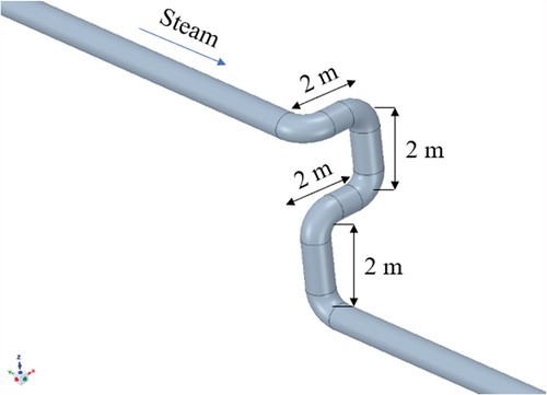
Figure 2. Front view of the pipe outlet.

Meanwhile, the establishment of the calculation model is based on the following assumptions:

1. The flow process is a three-dimensional steady-state process;

2. Ignoring the thickness of the wall, the boundary condition of the wall is set to a constant heat flux density (calculated according to the temperature difference between the inside and outside of the tube and the thermal conductivity of the wall insulation material);

3. Both gas and liquid phases are continuous fluids;

4. The steam does not contain non-condensable gas.

2.2. Mesh division and boundary conditions

2.2.1. Meshing

This paper uses the Meshing software to divide the mesh into the type of hexahedral. The mesh near the wall is encrypted with the consideration of the great change of temperature and velocity of the fluid caused by the steam condensation near the pipe wall. Table 1 lists the quality information of the mesh. And the details of the grids are shown in Figures 3 and 4.

Figure 3. Section and wall grid division diagram of the pipeline.

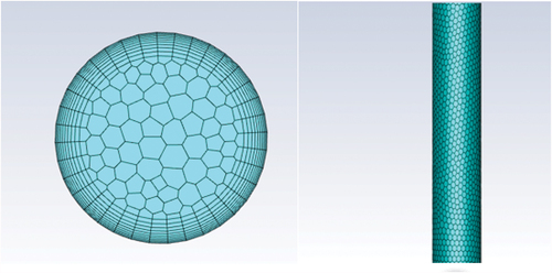
Figure 4. Details of the grid at the burst pipe.

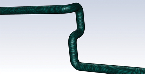
Table 1. Quality information of mesh

Mesh metric	Value
Orthogonal Quality	0.98451
The Max skewness	0.45812
Average skewness	3.25424e-2
Average aspect ratio	7.471
Average element quality	0.5122
Number of cells	2,833,124

2.2.2. Boundary condition setting

1. The import and export conditions of the model are set as follows:

Inlet: Given the mass flow rate (138.6 t/h) and temperature (553.15 K) of the inlet water steam. The steam velocity is evenly distributed on the inlet section. And the steam volume fraction at the inlet is 1. Note that the velocity is set to be uniformly distributed. Then, the relative turbulence intensity is calculated at the inlet according to the velocity and the pipe diameter.

Outlet: Given the steam pressure of the outlet section. The mass flow rate of the pipe outlet section is equal to the mass flow rate at the inlet.

1. The wall insulation condition is calculated as follows:

It is known that the thermal power plant adopts the following insulation methods: the outer wall of the pipe is covered with two insulation layers, while the insulation materials are aluminum silicate and asbestos wool. The thickness of the insulation layer is 80 mm. The thermal conductivity of aluminum silicate is about λ₁ = 0.1 W/(m·K), while the thermal conductivity of asbestos wool is λ₂ = 0.2 W/(m·K). The heat dissipated by the pipe network through the wall to the outside can be expressed as,

(1) $\mathrm{\varnothing }=\frac{2\pi l\left(t_{in}-t_{out}\right)}{\frac{ln\left(\frac{d_2}{d_1}\right)}{{\lambda }_1}+\frac{ln\left(\frac{d_3}{d_2}\right)}{{\lambda }_2}}$(1)

Therefore, the heat dissipation per unit area of the pipe can be obtained by dividing the calculated heat by the surface area. In this paper, the heat flux through the pipe is obtained at 228 W/m², which is used as the calculation boundary condition.

2.3. Model selection

2.3.1. Multiphase flow model

It is very important to track the phase interface to ensure the accuracy of the calculation and the reliability of the conclusion because the research object is the gas-liquid two-phase flow. The common multiphase flow models include the volume of fluid (VOF), Mixture model, and Eulerian model. The VOF model used here is contributed to the following reasons:

1. The VOF model can capture the phase-liquid interface and achieve high-precision simulation in phenomena such as stratified flow, free-surface flow, and large bubble flow. While the Mixture and Euler models are applied to sedimentation, particle suspension, and fluidized bed.

2. There is an obvious gas–liquid interface in a water hammer, and the vapor phase and the liquid phase do not mix. Thus, the VOF model that can be traced on the surface is selected as the multiphase flow model.

2.3.2. VOF model control equation

Based on the conservation laws of mass, energy, and momentum, the governing equations of the VOF model in this paper are as follows:

2.3.2.1. Continuity equation

(2) $\mathrm{\nabla }\cdot \left({ }_q{\alpha }_q{\rho }_q\right)=S_q+{\sum }_{p=1}^n\left(\stackrel{\cdot }{m_{pq}}-\stackrel{\cdot }{m_{qp}}\right)$(2)

where ${\alpha }_{\mathrm{q}}$ is the volume fraction of the q-phase fluid, ${\mathrm{S}}_{\mathrm{q}}$ is the volume source term, and ${\dot{\mathrm{m}}}_{\mathrm{p}\mathrm{q}}$ and ${\dot{\mathrm{m}}}_{\mathrm{q}\mathrm{p}}$ represent the mass transfer from the p phase to the q phase and the mass transfer from the q phase to the p phase, respectively. P phase and q phase mean the different phases in a phase transition process. In this work, p and q phases represent the phase gas and liquid.

Meanwhile, the volume fraction of each phase satisfies the following formula,

(3) $\left\{\begin{array}{c}{\sum }_{q=1}^n{\alpha }_q=1\\ {\sum }_{p=1}^n{\alpha }_p=1\end{array}\right.$(3)

2.3.2.2. The setting of physical properties

For the problem solved by the VOF model, the physical properties in the transport equation are determined according to the volume fraction of each phase (Ansys, 2018). Taking the density and viscosity in a two-phase flow as examples,

(4) $\left\{\begin{array}{c}\rho ={\alpha }_l{\rho }_l+{\alpha }_g{\rho }_g\\ \mu ={\alpha }_l{\mu }_l+{\alpha }_g{\mu }_g\end{array}\right.$(4)

There are only two forms of gas and liquid phases in this study, so the relationship between the gas and liquid phases can be expressed as,

(5) ${\alpha }_g=1-{\alpha }_l$(5)

2.3.2.3. Momentum equation

Each phase in the VOF model shares a set of momentum equations as,

(6) $\mathrm{\nabla }\cdot \left(\rho \stackrel{\rightharpoonup }{vv}\right)=-\mathrm{\nabla }\rho +\mathrm{\nabla }\cdot \left[\mu \left(\mathrm{\nabla }\stackrel{\rightharpoonup }{v}+\mathrm{\nabla }{\stackrel{\rightharpoonup }{v}}^T\right)\right]+\rho g+{\stackrel{\rightharpoonup }{F}}_v$(6)

ρ is the reference density, which specifically refers to the average value of the density in the entire space.

2.3.2.4. Energy equation

Only two forms of gas and liquid phases in this study, so the relationship between the gas and liquid phases can be expressed as,

(7) $\mathrm{\nabla }\cdot \left(\rho \stackrel{\rightharpoonup }{v}E\right)=\mathrm{\nabla }\cdot \left(k_{eff}\mathrm{\nabla }T\right)+S_h$(7)

k_eff means equivalent heat transfer coefficient; S_h is all volume heat source terms including radiation.

Moreover, the VOF model takes total energy and temperature as the mass average variables,

(8) $E={\sum }_{q=1}^n{\alpha }_q{\rho }_q{E}_q/{\sum }_{p=1}^n{\alpha }_q{\rho }_q$(8)

Eq is determined on the specific heat of phase q and the shared temperature.

2.3.3. Phase transition model

Lee model is a mechanical model based on physics, which is often used in VOF model. In this model, liquid-vapor mass transfer (evaporation and condensation) is controlled by the vapor-phase transport equation (Welch & Wilson, 2000), which is expressed by,

(9) $\mathrm{\nabla }\cdot \left({\alpha }_g{\rho }_g{\stackrel{\rightharpoonup }{V}}_g\right)={\dot{m}}_{lg}-{\dot{m}}_{gl}$(9)

Where v is the vapor phase; α_g is the vapor phase (gas) volume fraction; ρ_g is the vapor-phase density; ${\vec{V}}_g$ is the vapor phase velocity; ${\dot{m}}_{lg}and{\dot{m}}_{gl}$ are the mass transfer rates of evaporation and condensation, respectively.

The mass transfer rate of evaporation and condensation is calculated by the saturation temperature.

When T_l > T_sat (evaporation process):

(10) ${\dot{m}}_{lg}=coeff\cdot {\alpha }_l{\rho }_l\frac{\left(T_l-T_{sat}\right)}{T_{sat}}$(10)

When T_g<T_sat (condensation process):

(11) ${\dot{m}}_{gl}=coeff\cdot {\alpha }_g{\rho }_g\frac{\left(T_{sat}-T_g\right)}{T_{sat}}$(11)

coeff is an adjustment coefficient, which is defined as the reciprocal of the relaxation time and the value is 0.1. ${\alpha }_v$ and ${\rho }_v$ are the phase volume fraction and density, respectively.

2.3.4. Turbulence model

In terms of turbulence model selection, the k-epsilon model is the most widely used in industrial flow calculations. This model has a moderate amount of calculation and comparable accuracy and can be divided into three models (i.e. standard, RNG, and Realizable). The standard k-epsilon model ignores the intermolecular viscosity and is only suitable for completely turbulent flows. The RNG k-epsilon model can calculate low Reynolds number turbulence. However, it takes into account the rotation effect and the calculation accuracy of a strong swirl is low. Compared with the previous two models, the Realizable k-epsilon model contains another turbulent viscosity formula and corrected the dissipation rate. It can obtain good results for flow types such as swirl flow, channel flow, boundary layer flow with a directional pressure gradient (Welch & Wilson, 2000).

The object of this research is the high Reynolds number turbulence of high-temperature water vapor in the pipeline. Based on the characteristics of the above models, the Realizable k-epsilon turbulence model is selected to ensure the accuracy of wall-flow calculations.

2.3.5. Simulation condition

In summary, this paper mainly uses the VOF condensation model to simulate the condensation phenomenon in the process of steam transportation in a steady state. Table 2 lists the base condition of the CFD simulation.

Table 2. The base condition of the CFD simulation

Items	Value
Enviorment temperature	280.15 K
Steam inlet temperature	553.15 K
Steam inlet velocity	97.2, 138.6, 180 t/h
Steam inlet volume fraction	1.0
Steam inlet pressure	0.8433 Mpa
Pipe Inner Diameter	0.6 m
Insulation thickness	0.16 m
Total pipeline length before modification	821.85 m
Total pipeline length after modification	2629.8 m

2.4. Numerical method verification

The pressure-velocity correlation algorithm is the Coupled algorithm. The momentum equation and energy equation are discretely solved using the second-order upwind format, the pressure is discretely solved using the PRESTO! format and the interface between phases are reconstructed using the HRIC method. The error of energy is set to 10⁻⁶. And the error of other variables is set as 10⁻³. In the verification of grid independence, the thickness of the grid of the attached boundary layer is calculated using six thickness sizes of 1 cm, 3 cm, 4 cm, 6 cm, 7 cm, and 10 cm. The change in average heat transfer rate varies with the grid is shown in Figure 5. When the thickness of the attached grid is 6 cm and 7 cm with the number of grids are 2.83 million and 3 million, it is only a 0.78% difference (127,013.67 W vs 128005.41 W) between the heat transfer rate. Therefore, the grid size of the boundary layer in the subsequent calculation is 6 cm and the number of grids generated is 2.83 million.

Figure 5. The results of grid Independence verification.

3. Results and discussion

Based on the above models, this paper performs the analysis on the flow and heat transfer of the accident pipeline to further investigate the two-phase flow of the pipeline. Firstly, the simulation is conducted on the accident pipeline without modification to monitor the accumulation of condensed water for exploring the true cause of the pipe burst accident. Then, the modified and optimized pipeline network is analyzed again to verify the necessity of pipeline rectification and to explore the flow in the pipeline under different working conditions.

3.1. Accident pipeline simulation results

The total length of the accident pipeline before the modification is 821.85 m. According to the actual data provided by the enterprise, it is calculated that under the condition of an ambient temperature of 7°C, the wall heat dissipation is 352 kW and the temperature difference between inlet and outlet is about 4°C. Besides, the pressure drop in the pipe is about 35 kPa. Accordingly, the heat dissipation per unit length is 428.30 W/m and the temperature difference per unit length is 0.005°C/m. The pressure drop per unit length is about 43.41 Pa/m.

Figure 6 shows the distribution of condensation water in the pipeline. It can be seen that there is an obvious phenomenon of condensation water accumulation at the pipe elbow, which is almost the same as the location of the burst pipeline.

Figure 6. Distribution cloud diagram of condensate water inside the pipeline.

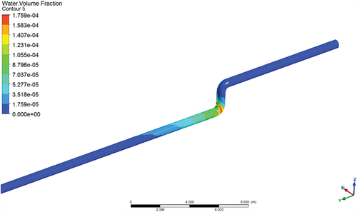
Then, a high-precision simulation is performed on the relevant details of the accident pipeline to obtain the water-phase volume fraction of the location where the condensed water appeared. The simulation result is shown in Figure 7. The highlighted part in the figure is the generated condensate.

Figure 7. Volume fraction diagram of water phase at steam condensation.

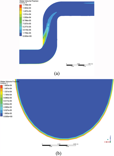
3.2. Specific analysis for the water hammer causes

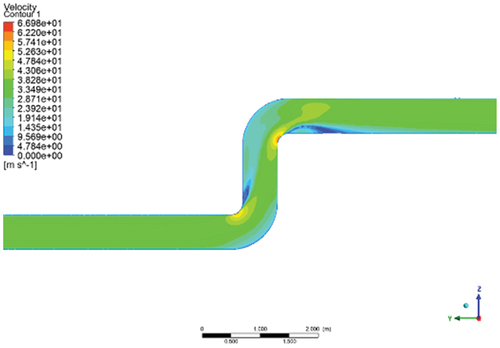
Referring to Figures 6 and 7, it can be seen that a liquid water film is formed on the lower wall of pipes in the original accident pipe network. The condensed water cannot be effectively discharged and accumulates at the burst tube under the action of flow. In detail, it is calculated that the total amount of condensed water formed by this pipeline is about 324 kg/h. Accordingly, the steam condensed to water and accumulated in the pipeline, which changes the velocity distribution in the pipe (as shown in Figure 8), which deteriorates the flow in the pipe and blocks the normal flow of steam in the pipe.

Figure 8. Velocity cloud diagram at condensation place.

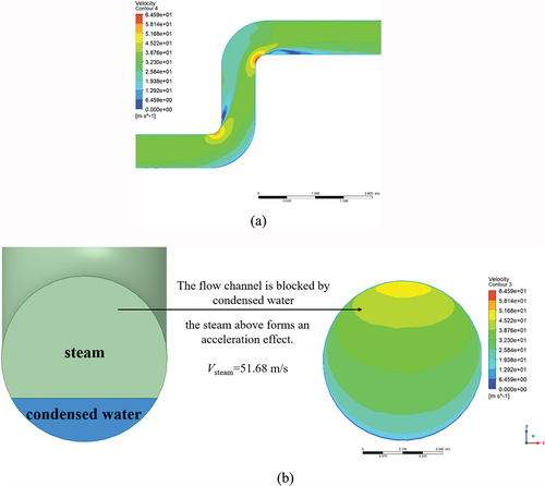
Near the vicinity of the burst pipe, due to the obvious accumulation of condensed water, the original steam flow channel is blocked, and the steam flow rate has a relatively obvious acceleration effect. Specifically, according to the original data, the steam velocity has surged from about 31 m/s to about 51 m/s. The flow in the pipe becomes a gas–liquid two-phase flow, which easily forms large air pockets and causes separation of the liquid column. At last, the water hammer will occur when the liquid column is recombined, eventually leading to a pipe burst accident.

To better explain the causes of pipe bursting, according to the relevant references, this study also calculated the sudden change of pressure during the water hammer process based on the Joukovsky water hammer pressure formula (Welch & Wilson, 2000; Xu et al., 2017),

(12) $\mathrm{\Delta }P=\rho a\left(V_0-V\right)$(12)

$\rho$ is the density of the liquid, a is the water hammer propagation velocity; V₀ is the initial velocity of the fluid, and V is the fluid velocity where the water hammer occurs.

According to the above empirical formula analysis, the sudden change of pressure caused by water hammer is mainly determined by the fluid density, the propagation velocity of the water hammer wave, the initial flow velocity, and the fluid velocity where the water hammer occurs. In this study, the proportion of condensed water in the flow channel directly determines the acceleration effect of steam. Table 3 shows the relationship between the proportion of condensed water in the flow channel and the change of water hammer pressure under the set conditions.

Table 3. The relation between water hammer pressure and proportion of condensate in pipeline

Proportion of condensed water (%)	Condensate flow(kg/h)	The steam flow rate (m/s)	Pressure change (MPa)
0	0.00	31.23	0
0.10	233.27	34.70	3.47
0.20	262.43	39.04	7.81
0.30	299.92	44.62	13.39
0.40	349.91	52.05	20.82
0.50	419.89	62.47	31.23
0.60	524.87	78.08	46.85

According to the water hammer pressure formula, the change in the water hammer pressure of the pipeline can be obtained when the amount of condensed water (the share of the condensed water in the flow passage) is different. As shown in Table 3, a large proportion of condensed water in the pipeline will cause a large steam velocity and water hammer pressure. Then, the possibility of pipeline water hammer also increases. It can be found that the amount of condensed water in this accident reached 324 kg/h, and the pressure increase reached nearly 20MPa at the same time, directly leading to the water hammer explosion accident.

3.3. Pipe network calculation after modification

After the burst pipeline accident, the original accident pipeline has been modified and the modified pipeline network has not experienced any bursts. Therefore, this section performs a simulation for the modified pipe network. The total length of the modified pipe network is 2629.8 m. It is calculated that the wall heat dissipation is 1127 kW and the overall pressure drop is about 101 kPa. The pressure drop and the heat dissipation per unit length before and after the modification are calculated as well, and the details are listed in Table 4. Referring to Table 4, the pressure drop per unit length after modification is lower than that before (38.64 Pa/m vs 43.41 Pa/m), which is mainly contributed to reducing the elbow part of the pipeline network. While the heat dissipation per unit length remains almost unchanged because of the same pipe insulations.

Table 4. Pressure drop and heat dissipation per unit length before and after the modification

	Simulation length	Pressure drop per unit length	Heat dissipation per unit length
Before the modification	821.25 m	43.41 Pa/m	0.428 kW/m
After the modification	2629.8 m	38.64 Pa/m	0.428 kW/m

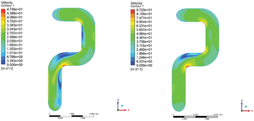
To confirm the effect of the modification, this paper conducts a detailed analysis of the pipeline after modification as well. The condensed water in the pipeline and the velocity distribution at the pipe burst place are shown in Figures 9 and 10. It can be seen that the phenomenon of condensed water accumulation inside the pipeline has been improved greatly. In addition, the speed distribution at the burst place is more uniform. The maximum flow velocity here is significantly lower than that before the modification, which greatly reduces the risk of water hammer and further verifies the benefits brought by the network modifications.

Figure 9. Distribution cloud diagram of condensate water inside the pipeline after modification.

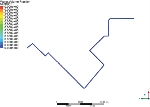
Figure 10. Velocity cloud diagram at pipe burst place.

3.4. Analysis of the modified pipeline network under variable conditions

In practical production, the working conditions of the water-steam pipe network are often restricted by external conditions. Thus, it is necessary to carry out calculations of pipe network operation under different working conditions. Accordingly, the steam flow rates of 97.2 t/h (70% reference conditions) and 180 t/h (130% reference conditions) are set to investigate the flow conditions of the pipeline and compared with the given reference conditions (138.6 t/h). The simulation results are shown in Figures 11–14.

Figure 11. Pressure cloud diagram at the burst tube place (side view) under different inlet mass flows (a) 97.2 t/h and (b) 180 t/h.

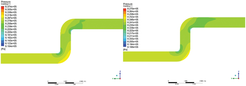
Figure 12. Velocity cloud diagram at the burst tube place (side view) under different inlet mass flows (a) 97.2 t/h and (b) 180 t/h.

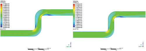
Figure 13. Pressure cloud diagram at the burst tube place (front view) under different inlet mass flows (a) 97.2 t/h and (b) 180 t/h.(a) 97.2 t/h. (b) 180 t/h.

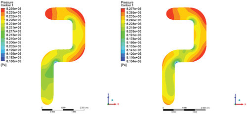
Figure 14. Velocity cloud diagram at the burst tube place (front view) under different inlet mass flows (a) 97.2 t/h and (b) 180 t/h.

As the pressure cloud diagrams (Figures 11 and 13) show, the pressure near the wall is significantly higher than the pressure in the mainstream area. As the velocity cloud diagrams (Figures 12 and 14) show, there are strong disturbances near the elbow with strong and high-speed motion. The steam will collide with the wall here and cause the flow to be turbulent. Moreover, it is also concluded that the pressure drop of the pipeline will change significantly when the flow rate changes. In detail, as Table 2 shows, the pressure drop of the normal flow after optimizing the pipeline is about 38.64 Pa/m. When the inlet mass flow is reduced by 30% (i.e. 97.2 t/h), the pressure drop is about 23.45 Pa/m, which is less than the normal pressure drop by 64.8%. When the inlet mass flow is increased by 30% (i.e. 180 t/h), the pressure drop increases to 69.45 Pa/m, which is higher than the normal pressure drop by 44.3%. In short, the stress load at the elbow of the pipe network will increase accordingly at a high steam flow rate. Thus, the control of the steam flow rate in the pipe must strictly follow the pipeline design standards.

4. Conclusions

This study carries out the flow and heat transfer analysis of a thermal power plant pipeline network that has suffered a burst pipe accident. The CFD method is employed and the analysis is performed for both the original and modified pipeline network. Based on the simulation results, the conclusions can be summarized as follows:

1. In the original accident pipeline, there are so many elbows that the pressure drop per unit pipeline is increased. The liquid water, condensed from the steam during the transportation process, occurs on the lower wall of the elbow near the accident and changes the velocity and temperature distribution in the pipe. In the accident pipeline, it is found that the steam velocity can reach up to 50 m/s, which is much beyond the steam velocity at the pipeline inlet. When the high-velocity gas strikes the elbow, it will lead to a sharp pressure change, which will ultimately endanger the safe operation of pipeline equipment.

2. In the modified pipeline network, there is no obvious phenomenon of condensed water accumulation because of the reduction of the elbow. It restrains the drastic changes in the flow field and makes the distribution of temperature, pressure, and velocity at the pipe burst place more uniform and reasonable.

3. The results of the modified pipeline network under variable conditions show that, when other conditions remain, the steam flow rate and the pipeline pressure drop are positively correlated. In other words, a greater flow rate will increase the load on the pipe network elbow, which indicates that the load should be kept as stable as possible in actual production.

In further work, the methodology used for phenomenon simulation can be combined with the flow or pressure measurements from one station, and then they can be used to localize possible defects in the system for actual operation simply and safety (Keramat et al., 2022).

Data availability statement

The data used to support the findings of this study are included in the article.

Disclosure statement

No potential conflict of interest was reported by the author(s).

Additional information

Funding

This work is supported by National Natural Science Foundation of China (No. 51506013) and Fundamental Research Funds for the Central Universities (2020CDJQY-A051).

References

- Allievi, L. (1925). Theory of water-hammer. Typography R. Garroni.
- Ansys, I. (2018). ANSYS fluent user’s guide, release 19.0. ANSYS Inc, Canonsburg.
- Bergant, A., Simpson, A. R., & Tijsseling, A. S. (2006). Water hammer with column separation: A historical review. Journal of Fluids and Structures, 22(2), 135–17. https://doi.org/10.1016/j.jfluidstructs.2005.08.008
- Beuthe, T. (1997). Review of two-phase water hammer. Proceedings of the Annual Conference-Canadian Nuclear Society, Canadian Nuclear Association.
- Boran, Z., Wuyi, W., & Mengshan, S. (2018). Experimental and numerical simulation of water hammer in gravitational pipe flow with continuous air entrainment. Water, 10(7), 928. https://doi.org/10.3390/w10070928
- Cai, S., Li, Q., Liu, C., & Zhou, Y. (2020). Evaporation of R32/R152a mixtures on the Pt surface: A molecular dynamics study. International Journal of Refrigeration, 113(1), 156–163. https://doi.org/10.1016/j.ijrefrig.2020.02.007
- Chaudhry, M. (2014). Applied hydraulic transients. Springer
- Chen, T., Ren, Z., Xu, C., & Loxton, R. (2015). Optimal boundary control for water hammer suppression in fluid transmission pipelines. Computers & Mathematics with Applications, 69(4), 275–290. https://doi.org/10.1016/j.camwa.2014.11.008
- Dudlik, A., & Prasser, H. M. (2009). Water hammer and condensation hammer scenarios in power plants using new measurement system. Forschung im Ingenieurwesen, 73(2), 67–76. https://doi.org/10.1007/s10010-009-0100-9
- Gruel, R. L., Huber, P. W., & Hurwitz, W. M. (1981). Piping response to steam-generated water hammer. Journal of Pressure Vessel Technology, 103(3), 219–225. https://doi.org/10.1115/1.3263394
- Gulawani, S. S., Joshi, J. B., Shah, M. S., Ramaprasad, C. S., & Shukla, D. S. (2006). CFD analysis of flow pattern and heat transfer in direct contact steam condensation. Chemical Engineering Science, 61(16), 5204–5220. https://doi.org/10.1016/j.ces.2006.03.032
- Hu, J., Liu, C., Li, Q., & Shi, X. (2018). Molecular simulation of thermal energy storage of mixed CO2/IRMOF-1 nanoparticle nanofluid. International Journal of Heat and Mass Transfer, 125, 1345–1348. https://doi.org/10.1016/j.ijheatmasstransfer.2018.04.162
- Hu, J., Liu, C., Liu, L., & Li, Q. (2018). Thermal energy storage of R1234yf, R1234ze, R134a and R32/MOF-74 nanofluids: A molecular simulation study. Materials, 11(7), 1164. https://doi.org/10.3390/ma11071164
- Jeon, S. S., Kim, S. J., & Park, G. C. (2011). Numerical study of condensing bubble in subcooled boiling flow using volume of fluid model. Chemical Engineering Science, 66(23), 5899–5909. https://doi.org/10.1016/j.ces.2011.08.011
- Joukowski, N. (1898). Memoirs of the imperial academy society of St. Petersburg. Proceedings of the American Water Works Association, 24, 341–424
- Keramat, A., Duan, H.-F., Pan, B., & Hou, Q. (2022). Gradient-based optimization for spectral-based multiple-leak identification. Mechanical Systems and Signal Processing, 171, 108840. https://doi.org/10.1016/j.ymssp.2022.108840
- Khamoushi, A., Keramat, A., & Majd, A. (2020). One-dimensional simulation of transient flows in non-newtonian fluids. Journal of Pipeline Systems Engineering and Practice, 11(3), 04020019. https://doi.org/10.1061/(ASCE)PS.1949-1204.0000454
- Kothandaraman, C. P., & Subramanyan, S. (2008). Fundamentals of heat and mass transfer. New Age International.
- Kubrak, M., Malesińska, A., Kodura, A., Urbanowicz, K., Bury, P., & Stosiak, M. (2021). Water hammer control using additional branched HDPE pipe. Energies, 14(23), 8008. https://doi.org/10.3390/en14238008
- Liu, L., Li, Q., Ju, F., Dong, X., & Yu, X. (2019). Numerical simulation and analysis of the vertical and double pipe soil - air heat exchanger. Thermal Science, 23(6 Part B), 3905–3916. https://doi.org/10.2298/TSCI170730001L
- Morales-Rodriguez, R. (2012). Thermodynamics - fundamentals and its application in science. Books on Demand
- Patel, G., Tanskanen, V., & Kyrki-Rajamki, R. (2014). Numerical modelling of low-Reynolds number direct contact condensation in a suppression pool test facility. Annals of Nuclear Energy, 71, 376–387. https://doi.org/10.1016/j.anucene.2014.04.009
- Peng, T., Li, Q., & Liu, C. (2016). Accelerated aqueous nano-film rupture and evaporation induced by electric field: A molecular dynamics approach. International Journal of Heat and Mass Transfer, 94, 39–48. https://doi.org/10.1016/j.ijheatmasstransfer.2015.11.053
- Peng, T., Li, Q., Xu, L., He, C., & Luo, L. (2017). Surface interaction of nanoscale water film with SDS from computational simulation and film thermodynamics. Entropy, 19(11), 620. https://doi.org/10.3390/e19110620
- Riasi, A., & Tazraei, P. (2017). Numerical analysis of the hydraulic transient response in the presence of surge tanks and relief valves. Renewable Energy, 107, 138–146. https://doi.org/10.1016/j.renene.2017.01.046
- Shah, A., Chughtai, I. R., & Inayat, M. H. (2010). Numerical simulation of direct-contact condensation from a supersonic steam jet in subcooled water. Chinese Journal of Chemical Engineering, 18(4), 577–587. https://doi.org/10.1016/S1004-9541(10)60261-3
- Tang, J., Zhang, Q., Zhang, Z., Li, Q., Wu, C., & Wang, X. (2022). Development and performance assessment of a novel combined power system integrating a supercritical carbon dioxide Brayton cycle with an absorption heat transformer. Energy Conversion and Management, 251, 114992. https://doi.org/10.1016/j.enconman.2021.114992
- Tian, W., Xiao, Z., Xiao, Z., & Xiao, Z. (2008). Numerical simulation and optimization on valve-induced water hammer characteristics for parallel pump feedwater system. Annals of Nuclear Energy, 35(12), 2280–2287. https://doi.org/10.1016/j.anucene.2008.08.012
- Urbanowicz, K., Stosiak, M., Towarnicki, K., & Bergant, A. (2021). Theoretical and experimental investigations of transient flow in oil-hydraulic small-diameter pipe system. Engineering Failure Analysis, 128, 105607. https://doi.org/10.1016/j.engfailanal.2021.105607
- Wang, L., Yue, X., Chong, D., Chen, W., & Yan, J. (2018). Experimental investigation on the phenomenon of steam condensation induced water hammer in a horizontal pipe. Experimental Thermal and Fluid Science, 91, 451–458. https://doi.org/10.1016/j.expthermflusci.2017.10.036
- Welch, S. W. J., & Wilson, J. (2000). A volume of fluid based method for fluid flows with phase change. Journal of Computational Physics, 160(2), 662–682. https://doi.org/10.1006/jcph.2000.6481
- Wood, F. (1937). The application of heaviside’s operational calculus to the solution of problems in water hammer. Trans ASME, 59, 707–713.
- Wu, C., Xu, X., Li, Q., Li, X., Liu, L., & Liu, C. (2021). Performance assessment and optimization of a novel geothermal combined cooling and power system integrating an organic flash cycle with an ammonia-water absorption refrigeration cycle. Energy Conversion and Management, 227, 113562. https://doi.org/10.1016/j.enconman.2020.113562
- Wu, C., Xu, X., Li, Q., Li, J., Wang, S., & Liu, C. (2020). Proposal and assessment of a combined cooling and power system based on the regenerative supercritical carbon dioxide Brayton cycle integrated with an absorption refrigeration cycle for engine waste heat recovery. Energy Conversion and Management, 207, 112527. https://doi.org/10.1016/j.enconman.2020.112527
- Xu, J., Xie, J., He, X., Cheng, Y., & Liu, Q. (2017). Water drop impacts on a single-layer of mesh screen membrane: Effect of water hammer pressure and advancing contact angles. Experimental Thermal and Fluid Science, 82, 83–93. https://doi.org/10.1016/j.expthermflusci.2016.11.006
- Zaltsgendler, E., Tahir, A., & Leung, R. K. (1996). Condensation-induced water hammer in a vertical upfill pipe. Transactions of the American Nuclear Society.
- Zhang, H., Liu, C., Xu, X., & Li, Q. (2017). Mechanism of thermal decomposition of HFO-1234yf by DFT study. International Journal of Refrigeration, 74, 397–409. https://doi.org/10.1016/j.ijrefrig.2016.10.020
- Zhou, Y., Li, Q., & Wang, Q. (2019). Energy storage analysis of UIO-66 and water mixed nanofluids: An experimental and theoretical study. Energies, 12(13), 2521. https://doi.org/10.3390/en12132521