Predicting cervical cancer biopsy results using demographic and epidemiological parameters: a custom stacked ensemble machine learning approach

Abstract

The human papillomavirus (HPV) is responsible for most cervical cancer cases worldwide. This gynecological carcinoma causes many deaths, even though it can be treated by removing malignant tissues at a preliminary stage. In many developing countries, patients do not undertake medical examinations due to the lack of awareness, hospital resources and high testing costs. Hence, it is vital to design a computer aided diagnostic method which can screen cervical cancer patients. In this research, we predict the probability risk of contracting this deadly disease using a custom stacked ensemble machine learning approach. The technique combines the results of several machine learning algorithms on multiple levels to produce reliable predictions. In the beginning, a deep exploratory analysis is conducted using univariate and multivariate statistics. Later, the one-way ANOVA, mutual information and Pearson’s correlation techniques are utilized for feature selection. Since the data was imbalanced, the Borderline-SMOTE technique was used to balance the data. The final stacked machine learning model obtained an accuracy, precision, recall, F1-score, area under curve (AUC) and average precision of 98%, 97%, 99%, 98%, 100% and 100%, respectively. To make the model explainable and interpretable to clinicians, explainable artificial intelligence algorithms such as Shapley additive values (SHAP), local interpretable model agnostic explanation (LIME), random forest and ELI5 have been effectively utilized. The optimistic results indicate the potential of automated frameworks to assist doctors and medical professionals in diagnosing and screening potential cervical cancer patients.

Keywords:

• cervical cancer
• diagnosis
• Explainable Artificial Intelligence
• machine learning
• ANOVA
• stacking

Public Interest Statement

Cervical Cancer is a dangerous disease and causes a large number of deaths all around the world. If the cancer is screened at an early stage, treatments are available. Artificial Intelligence and machine learning are normally used for disease screening. In this research, we use Explainable Artificial Intelligence techniques to predict the biopsy results. Explainable Artificial Intelligence makes the model more precise and interpretable. A custom multi-layer stacking model is used to cervical cancer classification in this study. This article involves multi-disciplinary research and aids researchers from Computer Science, Biomedical and Medical back grounds. The models can be further used to diagnose other dangerous diseases such as COVID-19, AIDS, monkey pox and others. We understand the importance of various epidemiological and demographic parameters in cervical cancer diagnosis such as age, intra-uterine devices, contraceptives and others. The models can be deployed in all hospitals to screen potential cervical cancer patients.

1. Introduction

Cervical cancer effects a lot of women worldwide and causes a large number of fatalities in under developed countries (L Yang et al., 2020). As of 2021, an estimated case of 14,280 has been recorded by the United States of America alone (Arbyn et al., 2022). Human papillomavirus (HPV) is responsible for this deadly cancer in most cases (more than 95%) (Cohen et al., 2019). This gynaecological cancer develops over time, and normal cells require years to progress from a non-cancerous lesion to a dreaded cancer cell. Nonetheless, it is well accepted that a preliminary diagnosis of malignant lesions can prevent cancer growth in approximately 90% of cervical cancer patients (Zhu et al., 2022). HPV vaccines are also available in most countries. Regular screening programs such as cytology, pap smear and digital colposcopy tests can help prevent this cancer (Arbyn et al., 2022). Furthermore, the affected tissues can be successfully removed if it is identified at an early stage. Later stage symptoms include increased vaginal discharge, postcoital bleeding, pelvic pain and excessive bleeding during menstruation (Z Alam et al., 2022). However, none of the above symptoms is observed in this dangerous disease’s early stages. Furthermore, in many underdeveloped countries, large-scale screening programs’ facilities are insufficient and scarce. Patients also have poor adherence to regular testing due to a lack of understanding of the disease (Brüggmann et al., 2022).

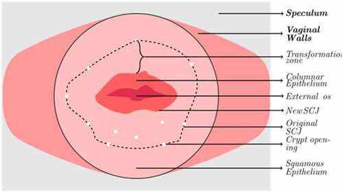
Currently, this cancer diagnosis involves two tests: First, the patient is required to undergo a cytology test called the pap smear or Papanicolaou’s test (da Silva et al., 2022). In this test, cells are gently removed from the cervix and the surrounding regions with a tiny brush to be examined under a powerful microscope. Cell abnormalities and cancer cells can be easily identified using this method. The next step is to conduct a thorough colposcopy exam (Ren et al., 2022). The protocol for this procedure involves four significant steps. The first step involves the observation of columnar and squamous epithelium using a saline solution under the influence of a magnifier lens. Abnormalities in the tissue are observed in the squamous epithelium. Generally, it is pink in colour. Crypt apertures and nabothian follicles are the critical points of interest. These artefacts define the transformation zone’s external boundary. The SQJ characterizes the inner perimeter. The full view of the region of interest is sometimes impossible to view from a source since the SQJ may retract into the canal. The columnar epithelium has a dark red appearance with complicated patterns. A green filter can then be attached to the colposcope to enhance the vision of the vasculature by maximizing the contrast. Reticulated and hair-pin-shaped capillaries are the two structures observed in this stage. These unique patterns can only be found in specific regions in the cervix, as described in Figure 1. In the next step, the cervix is observed under the influence of acetic acid solution (5%). This idiosyncratic procedure was first performed by Hans Hinselmann in 1925 (Yoon et al., 2022). The epithelium tissues are observed once again. The clinicians can easily distinguish the change in the appearance of the squamous and columnar epithelium tissues due to the presence of acid. During this phase, precancerous lesions might also be seen. The last step involves the physician applying Lugol’s solution to the cervix. This procedure is called as the Schiller’s test (Jaya & Latha, 2022). The healthy cervical and vaginal tissues become black or brown. Abnormal entities such as cervical polyps do not get stained by the iodine solution. As a result, the test strengthens the ability to distinguish between normal and aberrant transformation zone regions. The abnormal development of cells on the cervix characterizes cervical cancer. The biopsy result of colposcopy is used to diagnose cervical cancer in most cases. However, they can lead to false positive and negative results (Beer, 2021). The inaccurate results are dangerous since the patient does not receive appropriate treatments and can lead to a severe prognosis.

Figure 1. Internal structure of the cervix.

Several studies have found significant changes in the risk of contracting cancer at various age levels. This cancer can be easily prevented, yet most women are unaware of the aetiology, health risks, prevention and management of cervical cancer due to their background and education levels. Cervical cancer is rare in developed countries, and low-income nations account for almost 95% of cervical cancer mortality (Alquran et al., 2022). Another prominent reason is the HPV infection, which spreads through sexual contact. As a result, the age during first sexual contact, the number of sexual partners, and the use of contraceptives have all been linked to cervical cancer (Al-Hashem et al., 2021). If these factors are managed, the occurrence of this malignant tumour can be minimized. Regular cervical cancer screening can prevent infections and is also an effective measure for clinical management of potential cancer patients (Arbyn et al., 2022; Terasawa et al., 2022). There is also a pressing need to identify alternative approaches to diagnosing early-stage cancer. Obstetrics and socio-demographic profiles have been widely used to find patients at risk of contracting this carcinoma. Furthermore, the genetic, epidemiological and clinical data have various interesting patterns that can be easily understood by Artificial Intelligence (AI).

Artificial Intelligence is one of the most trending subjects in today’s world (Alsharif et al., 2021). It comprises various sub-disciplines such as modelling, simulation, statistics, machine learning, deep learning and algorithms (Alqudah, Qazan, et al., 2021). Machine learning (ML) is a subset of AI which involves training a dataset and predicting results. It also substantially contributes to academic and clinical research (Khanna et al., 2022). Medicine, Engineering, biomedical, sociology, psychology and many other domains use ML in their applications. According to published studies, ML is already utilized in face recognition, drug development, automated robots, drone engineering, big data engineering, customer prediction and many more (Alqudah & Alqudah, 2022a; Masad et al., 2021, A Alqudah et al., 2021). It is extensively used in battling the recent pandemic too (Alqudah & Alqudah, 2021a). The ML framework used in this research for predicting biopsy results in cervical cancer patients can lead to a better and more trustworthy diagnosis. The outcomes obtained by these models can be further compared with the results obtained by the actual biopsy test for better validation.

The following are the article’s key findings and contributions:

• A comprehensive review of various existing machine learning applications that detect cervical cancer.

• A deep exploratory data analysis which identifies vital patterns in the patient’s epidemiological and demographic data.

• The utilization of various ML models to ensure the trustworthiness of the results obtained. These models are further “STACKED” on various levels to increase the accuracy.

• The effect of Borderline-SMOTE (Synthetic Minority Oversampling Technique) (A data balancing technique) on the results obtained by the models.

• The utilization of Explainable Artificial Intelligence (SHAP, LIME, random forest and ELI5) for better explainability and interpretability. These techniques make the models more understanding to clinicians and hospital staff.

• Further information about the various factors critical in diagnosing cervical cancer from a medical perspective.

The dataset considered for this research was acquired from Hospital Universitario de Caracas, Venezuela (Fernandes et al., 2017). This data consists of 35 risk factors and biopsy results of 859 patients tested for this dangerous disease. A stacked machine learning methodology was adapted in this study to predict biopsy results of patients tested for cervical cancer (Džeroski & Ženko, 2004). These models were efficiently trained with data and analyzed using several evaluation metrics. Data balancing was performed using a “Borderline-SMOTE” technique before model training (Han et al., 2005). In the beginning, the data was subjected to pre-processing too. The results of specific cervical cancer tests such as Hinselmann’s and cytology were also considered for this research. The several stages of this carcinoma, along with the survival rate, are described in Table 1. The rest of the article is as follows: A review of similar literature is conducted in section 2. Section 3 describes materials and methods, followed by results in section 4. The article concludes in section 5.

Table 1. Cervical cancer various stages

Stage	Symptoms	Five-year survival rate
Stage 0	Carcinoma present in situ. The cervix’s innermost membrane contains malignant cells	97–100%
Stage 1	Cervical cancer that is localized to the cervix itself.	81–96%
Stage 2	The malignancy has progressed beyond the uterus, although not to the pelvic sidewalls or the lower part of the vaginal cavity.	65–87%
Stage 3	Cancer cells spread to lower third of the vaginal canal and side walls. The kidneys start to malfunction as well.	35–50%
Stage 4	The cancer had migrated beyond the pelvis. The cancerous cell spread to the rectum and bladder too.	15–20%

2. Related literature

Several researchers have used the applications of AI in diagnosing cervical cancer. The preliminary screening of this disease is vital to mitigate a severe prognosis. The AI models can further confirm the biopsy results and prevent wrong outcomes. In this section, we describe the latest research by engineering and medical professionals worldwide.

In a research article by Lu et al. (Lu et al., 2020), ensemble machine learning was explored to assist in diagnosing cervical cancer. A voting strategy was used, which combines the results of various classifiers. Validation was further improved using a gene-assistance module. The proposed module achieved an accuracy of 83.16%. However, the recall, precision and f1-score were extremely poor, with 28.35%, 51.73% and 32.80%, respectively. The cervical cancer risk for Indian patients were explored by Kaushik et al. (Kaushik et al., 2021). The dataset included demographic and clinical parameters of both cancer and non-cancer patients. Cytokine gene variants were explored too. Among various algorithms, logistic regression obtained optimal results with an accuracy of 82.25%. The article concluded that cytokine parameters could be efficiently used as bioMarchkers to predict the biopsy results. Deepa et al. (Deepa, 2021) used neural networks to predict the fourth dangerous cancer that women suffer from. Four target variables were considered, and ANN performed slightly better than the machine learning models. For the biopsy result, the accuracy, precision and f1-score obtained by the models were 85%, 70% and 84%, respectively.

Yang et al. (W Yang et al., 2019) used machine learning to identify various risk factors that may lead to cervical carcinoma. A Venezuelan dataset was used, which contained the biopsy results of 858 patients along with four target variables. Multi-layer perceptron (MLP) and random forest were the algorithms utilized. For biopsy prediction, the highest accuracy obtained was 88.7%. According to feature importance, the most important parameters were age, number of sexual partners, age, hormonal contraceptives, and sexually transmitted diseases. In another research, machine learning was again used to predict cervical carcinoma (Akter et al., 2021). Three machine learning algorithms were implemented: random forest, xgboost and decision tree. The maximum accuracy was 93.33%. These algorithms were further compared with other research to prove their novelty and explainability. Thirty-two risk factors were considered for cervical carcinoma detection in (Deng et al., 2018). Among all the machine learning models used, xgboost was more reliable. Further, to achieve data balancing, the SMOTE technique was effectively utilized. The accuracy, sensitivity, specificity and f1-score obtained by the optimal classifiers were 95.59%, 93.92%, 97.25% and 96%, respectively.

Fernandes et al. (Fernandes, Cardoso, et al., 2018) used automatic decision support techniques to identify cervical cancer using digital colposcopies. Here, the dataset consisted of images. Quality assessment, image segmentation of cervical tissues, registration of images, detection of abnormal cells and classification were all performed in this research. However, the articles do not mention the performance metrics. Various classifiers used the selective feature approach technique to detect cervical cancer (Chauhan & Singh, 2022). Univariate analysis and recursive feature elimination were used for data preprocessing. Further, models were tested and validated. Among all the classifiers, random forest proved to be superior. To predict the biopsy results, the accuracy, precision, recall, f1-score and AUC obtained by the best performing models were 98.53%, 98.07%, 100%, 97% and 99%, respectively.

Explainable AI and ensemble ML algorithms were used to predict cervical cancer biopsy results (Curia, 2021). SHAP and LIME were used for explainability and interpretability. The ensemble classifier obtained accuracy, precision and recall of 94%, 94% and 67%, respectively. Clinical explainability was further achieved. Finally, Jahan et al. (Jahan et al., 2021) used machine learning to diagnose this deadly cancer. Eight classification algorithms were used for this purpose. The top 25 features were considered, and the MLP algorithm performed the best. The accuracy, precision, recall and f1-score were 97.40%, 97%, 97.4% and 97.2% respectively. Other research articles are compared in Table 2.

Table 2. Various researches that diagnose cervical cancer using machine learning approaches

Reference	Dataset Source	Dataset Size	Number of Features Chosen	Models used	Accuracy	Sensitivity	Specificity	AUC	Critical Analysis/ Findings
(Nithya & Ilango, 2019)	Hospital Universitario de Caracas in Caracas, Venezuela	858 Patients	36 attributes	C5.0, rpart, KNN, random forest, SVM	97%	-	-	91%	The use of Boruta algorithm to assist random forest algorithm.
(Fernandes, Chicco, et al., 2018)	Hospital Universitario de Caracas in Caracas, Venezuela	858 Patients	36 attributes	Various ML methods.	-	-	-	68%	Joint dimensionality reduction with accurate classification
(Ijaz et al., 2020)	Hospital Universitario de Caracas in Caracas, Venezuela	858 Patients	36 attributes	Various ML methods	96%	97%	94%	-	Outlier detection using DBSCAN.
(Suman & Hooda, 2019)	Hospital Universitario de Caracas in Caracas, Venezuela	858 Patients	36 attributes	Various ML methods	96%	-	-	95%	The use of decision stump algorithms. MCC was used as a performance metric.
(Lee et al., 2021)	Hospital Universitario de Caracas in Caracas, Venezuela	858 Patients	36 attributes	Various ML methods	-	-	-	-	In-depth mathematical intuition for cervical cancer diagnosis.
(Soğukkuyu & Ata, 2022)	Hospital Universitario de Caracas in Caracas, Venezuela	858 Patients	36 attributes	Various ML methods	97%	-	-	-	Novel ensemble methods
(Aloss et al., 2022)	Hospital Universitario de Caracas in Caracas, Venezuela	858 Patients	36 attributes -	Various ML methods	97%	-	-	-	The use of crow search algorithm for feature selection

3. Materials and methods

3.1. Dataset description

The entire data was acquired from the repository at the University of California, Irvine (UCI). The data was initially gathered at a Venezuelan medical facility, Universitario Hospital de Caracas, in early 2017 (Fernandes et al., 2017). The details of 858 patients tested for cervical cancer were included. Thirty-five essential features, which include patient demographics, critical medical records and behavioral aspects and the target variable “Biopsy results”, are present in the tabular form. The details of other relevant tests, such as the Hinselmann’s, Schiller’s, and Cytology tests are also present. Colposcopy with diluted acetic acid is used in the Hinselmann’s test, colposcopy with Lugol’s iodine solution is used in the Schiller’s test and the pap smear test is used in Cytology. A malignantly infected target is labelled as a “1” and a benign target is labelled as a “0”. The values for all features are floating, integer or Boolean datatypes. Multiple null values exist in the database due to a number of patients dodging questions due to privacy issues. Table 3 describes various attributes present in this dataset, including the number of missing values.

Table 3. Description of the dataset

Feature	Range (Min: Max)	Datatype	Missing Values	Description	Feature	Range (Min: Max)	Datatype	Description	Missing Values
Biopsy result: Target variable	0:1	Boolean	0	Result obtained after the biopsy test	STD- Vulvo Perineal Condylomatosis	0:1	Boolean	It indicates the presence of this particular STD.	105
Cytology test	0:1	Boolean	0	Result obtained after the cytology test	STD- Vaginal Condylomatosis	0:1	Boolean	It indicates the presence of this particular STD.	105
Schiller’s test	0:1	Boolean	0	Result obtained after the Schiller’s test	STD- Cervical Condylomatosis	0:1	Boolean	It indicates the presence of this particular STD.	105
Hinselmann’s test	0:1	Boolean	0	Result obtained after the Hinselmann’s test	STD- HPV	0:1	Boolean	It indicates the presence of this particular STD.	105
Age	13:84	Integer	0	Age of the patient	STD: Hepatitis B	0:1	Boolean	It indicates the presence of this particular STD	105
Age during the first sexual intercourse	10–32	Integer	7	Age during the first sexual intercourse	STD: HIV	0:1	Boolean	It indicates the presence of this particular STD.	105
Number of sexual partners	0–28	Integer	26	The number of sexual partners	STD: AIDS	0:1	Boolean	It indicates the presence of this particular STD.	105
Pregnancies	0:11	Integer	56	The number of pregnancies	STD: Mollusc-um Contagio-sum	0:1	Boolean	It indicates the presence of this particular STD.	105
Smokes (years/pack)	0:37	Integer	13	It represents the sum of cigarette packets smoked by the patient in a year	STD: Genital herpes	0:1	Boolean	It indicates the presence of this particular STD	105
Smokes (Years)	0:37	Integer	13	Time in years since the patient started smoking	STD: Pelvic Inflammatory	0:1	Boolean	It indicates the presence of this particular STD	105
Smokes	0:1	Boolean	13	It indicates whether the patient smokes or not	STD: Syphilis	0:1	Boolean	It indicates the presence of this particular disease	105
Hormonal Contraceptives (years)	0:30	Integer	108	The number of years since the patient is using hormonal contraceptives	STD: Number of Diagnosis	0:3	Integer	Total number of times tested.	707
Hormonal Contraceptive	0:1	Boolean	108	It indicates whether the patient uses contraceptive or not	STD: Time since last diagnosis	1:22	Integer	Total number of years since last diagnosis	707
Intra-uterine device (IUD)(years)	0:19	Integer	117	The number of years since the patient is using IUD’s	STD: Time since first diagnosis	1:22	Integer	Total number of years since the first diagnosis	0
IUD	0:1	Boolean	117	It indicates whether the patient used IUD’s or not	Dx	0:1	Boolean	It indicates whether HPV, Cervical intraepithelial neoplasia (CIN) or cancer are present	0
Sexually transmitted diseases (STD’s)	0:1	Boolean	105	It indicates whether the patient has STD.	Dx: HPV	0:1	Boolean	It indicates the presence of this disease	0
Number of STD’s	0–4	Integer	105	The number of STD’s present.	Dx: Cin	0:1	Boolean	It indicates the presence of this disease	0
STD- Condylomatosis	0:1	Boolean	105	It indicates whether the patient has Condylomatosis	Dx: Cancer	0:1	Boolean	It indicates the presence of this disease	0

3.2. Data preprocessing

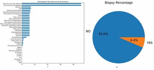
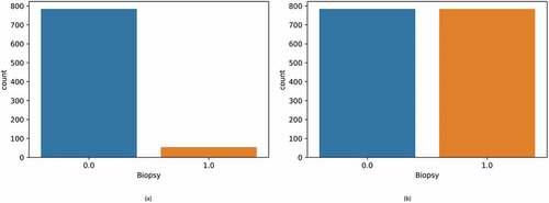
The initial data, which consisted of 858 rows and 36 columns, had many null values. These missing values were represented using the “?” symbol. Initially, this symbol was replaced with “NaN” for ease of processing. Figure 2a displays the null values present in the dataset in the form of a bar graph. From the figure, it can be observed that the parameters “STD: Time since the first diagnosis” and “STD: Time since last diagnoses” had many null values. Replacing these null values would render the classifier useless. Hence, the above two parameters were dropped. Most patients were diagnosed as non-cancerous after the biopsy test and only 6.4% had cervical cancer, as per Figure 2b.

Figure 2. (a) Bar graph showing the percentage of null values in the dataset (b) The percentage of biopsy positive and biopsy negative results.

There are three principal approaches to coping with null values, each with its model dynamics and characteristics. The first way is to keep the sparsity in the data. This strategy has two significant drawbacks. The majority of AI algorithms do not work with null values. Some classifiers will fail during training because they employ a parameter estimator method that necessities the usage of a dense matrix. The secondary issue is that the models need to have some “variance” to “learn” about the essential attributes in the data. A few independent attributes lose their “protagonism” too. As a result, the attribute does not influence the output, regardless of the field of application. The benefit of this strategy is that the data can be utilized immediately without the need for preprocessing. Another viable option is the classifier-based attribute imputation. Most biological and AI tools use the “singular value decomposition” to deal with null values. When there are many cases, classifier-based matrix completion techniques can help. The most significant disadvantage of this method is the amount of computing power necessary to find the best possible solution using hyperparameter tuning. This can be a hurdle when the data is vast. Although these methods have recently improved in terms of efficiency and parallel processing, there is still scope for improvement. The third method is to use descriptive statistics to replace the missing values. The most typical metrics for this task are mean, median and mode. These values get more accurate as the number of cases increases. However, skewed results can be obtained if the models generate significant bias. We chose the third method for this study since it is relatively simple. The median replaced numerical attributes, and categorical attributes were replaced by the distribution mode. Mean value imputation was avoided since they are severely affected by outliers.

Feature scaling is a strategy for fitting the dataset’s independent attributes into a specified range (Chandrashekar & Sahin, 2014). It addresses significantly changing values, magnitude and units during initial data preprocessing. If the normalization is not performed, an AI algorithm prefers larger values, irrespective of the units used. Generally, there are two ways to scale the data: (a) Standard scalar uses the standard normal distribution. All the means of the attributes are made zero, and the variance is scaled to one (b). The Min-Max scalar converts all the data in the range from zero to one. If negative values are present, the scaling is performed between “-1” and one. In this study, the attributes were normalized using the standard scalar method.

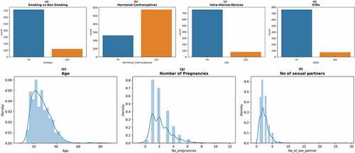
After initial data preprocessing, univariate analysis was conducted to understand more about the data. The attributes were analyzed visually using a bar plot and probability density function for both the classes present in the biopsy label. Figure 3 describes various count and density plots. From Figure 3a, it can be inferred that most patients did not smoke. Referring to birth control habits, most patients used pills and other hormonal contraceptives. Only a few opted for intra-uterine devices. This is due to the fact that these pills are readily available in medical dispensaries. This can be observed from Figure 3b and c. Further, from Figure 3d, it can be seen that most patients did not have any sexually transmitted diseases. From Figure 3e, we were able to infer that most patients were in the age group of 20 to 40. From Figure 3f, it can be inferred that most patients experienced between one to four pregnancies. From Figure 3g, it can be inferred that most patients had 1–5 sexual partners.

Figure 3. Count plots and density plots (a) The number of patients who smoke (b) The number of patients who use hormonal contraceptive (c) The number of patients who use intra-uterine devices (d) The number of patients who have sexually transmitted diseases (e) Patient age distribution (f) The number of pregnancies (g) The number of sexual partners.

After univariate analysis, multivariate analysis was performed. Figure 4a shows a box plot to understand the relationship between age and age during first sexual intercourse on biopsy results. From the figure, it can be inferred that sexual intercourse at a young age (14–19 years) can result in a positive biopsy result. In Figure 4b, a box plot is used to understand the relationship between age, the number of sexual partners and the biopsy result. The figure shows that the chances of getting diagnosed with cervical cancer increase when the number of sexual partners increases. In Figure 4c, a box plot is used to understand the significance of the age and the number of pregnancies on the biopsy result. From the figure, it can be observed that there is no clear evidence that the number of pregnancies increases the chance of cancer. Patients with zero pregnancies have also tested positive. Figure 4d was used to determine the effect of smoking and the number of pregnancies on the biopsy result. It was found that the combination of a patient smoking and increased pregnancies might lead to cervical cancer. It can also be inferred that cervical cancer affects patients who do not smoke too. Figure 4e and f were used to determine the effect of hormonal contraceptives and Intra uterine devices (IUD) on the biopsy result. From the figures, it can be inferred that using these birth control measures might lead to cervical cancer. It can also be seen that patients who used hormonal contraceptives and had a higher age (30 and above) were more likely to test positive for the biopsy test. Patients who used IUDs and were older (40 and above) were also more likely to develop cervical cancer. From all the above figures, it can be inferred that age is a crucial factor. The chances of getting diagnosed with cervical cancer increase with the patient’s age.

Figure 4. Multivariate analysis using box plots.

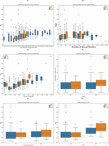
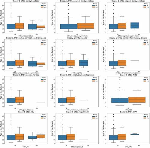
Figure 5 shows the relationships between various STDs, age and their impact on the biopsy result. It can be inferred that higher-age patients can contract cervical cancer. The effect of induced STDs on the biopsy result cannot be predicted since the data is insufficient and suffers from data imbalance between the classes.

Figure 5. The impact of STD’s on the biopsy result.

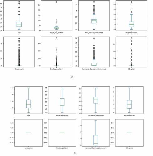
From the above boxplots, it can be seen that there are many outliers. These values reduce the accuracy of the model and reduce its performance. The interquartile range technique (IQR) was used to remove the outliers in this research. Deviations above the higher whiscus value have been capped at the 75% percentile (Upper whiscus, Q3), while deviations below the 25% percentile (Lower whiscus, Q1) have been capped at the lower whiscus itself. After analysis, the data was prepared for feature selection. Figure 6 shows boxplots before and after outlier treatment. After data-preprocessing, it is imperative to choose the correct number of features. The following section discusses the various feature selection techniques.

Figure 6. The presence of outliers in data. (a) Outliers before IQR treatment (b) After IQR treatment (Outliers removed).

3.3. Feature selection

The extraction of essential features from the entire dataset to obtain better performance is called feature selection (Chandrashekar & Sahin, 2014; J Li et al., 2017). This separates the relevant and useful features from the initial high dimensional data, which contains many unnecessary features that might reduce the accuracy of the classifier. In this research, we have used a statistical technique called “ANOVA” (Analysis of Variance) as a feature selection technique. ANOVA has evolved into a parameterized method that can be utilized to equate “class means” using a given attribute for the data (Langenberg et al., 2022). According to the null hypothesis, if there is no compelling variation between the means of classes for a particular attribute, that attribute can be removed. According to the alternative hypothesis, the attribute can be considered for the final model if there is a significant difference in their means. A p-value that is dependent on the attributes is also considered. A p-value is chosen by a parameter called “F-measurement”. The F value is defined as follows. Algorithm 1 denotes the steps which are required to perform feature selection using ANOVA.

The variation among classes is defined as:

The total sum of square errors (SE) among the two labels (0-non-ICU, 1-ICU)

(1) $SE=n_0{\left({\mu }_0-\mu \right)}^2+n_1{\left({\mu }_1-\mu \right)}^2+\hspace{0.17em}...$(1)

$n_0,n_1\to \mathrm{S}\mathrm{a}\mathrm{m}\mathrm{p}\mathrm{l}\mathrm{e}\mathrm{s}\mathrm{o}\mathrm{f}\mathrm{t}\mathrm{w}\mathrm{o}\mathrm{c}\mathrm{l}\mathrm{a}\mathrm{s}\mathrm{s}\mathrm{e}\mathrm{s}$

$\mu \to \mathrm{M}\mathrm{e}\mathrm{a}\mathrm{n}\mathrm{o}\mathrm{f}\mathrm{t}\mathrm{h}\mathrm{e}\mathrm{e}\mathrm{n}\mathrm{t}\mathrm{i}\mathrm{r}\mathrm{e}\mathrm{f}\mathrm{e}\mathrm{a}\mathrm{t}\mathrm{u}\mathrm{r}\mathrm{e}$

${\mu }_0,{\mu }_1\to M\mathrm{e}\mathrm{a}\mathrm{n}\mathrm{o}\mathrm{f}\mathrm{t}\mathrm{h}\mathrm{e}\mathrm{r}\mathrm{e}\mathrm{s}\mathrm{p}\mathrm{e}\mathrm{c}\mathrm{t}\mathrm{i}\mathrm{v}\mathrm{e}\mathrm{c}\mathrm{l}\mathrm{a}\mathrm{s}\mathrm{s}\mathrm{e}\mathrm{s}\mathrm{f}\mathrm{o}\mathrm{r}\mathrm{t}\mathrm{h}\mathrm{e}\mathrm{f}\mathrm{e}\mathrm{a}\mathrm{t}\mathrm{u}\mathrm{r}\mathrm{e}$

Degree of freedom (DF) within the two labels

(2) $DF=TotalClasses-1$(2)

The total mean square error (MS) between the two dichotomous labels

(3) $MS=SE/DF$(3)

The squared error sum among classes is defined as intra-class variation (ICV)

(4) $ICV=\left(n_0-1\right){\sigma }_0^2+\left(n_1-1\right){\sigma }_1^2+\dots$(4)

${\sigma }_0,{\sigma }_1\to Standarddeviationamongthetwoclasses$

Degree of freedom with the two classes (DFC)

(5) $DFC=Sumofsamples-Sumofclasses$(5)

Mean squared error within labels (MSL)

(6) $MSL=ICR/DFC$(6)

F Statistic is defined as

(7) $F=MS/MSL\hspace{0.17em}$(7)

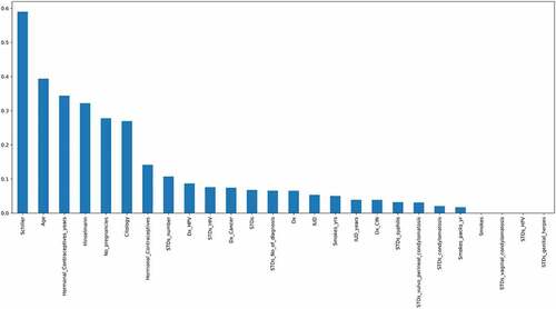
The top 18 features were chosen by using this feature selection approach. The features are as follows: “ Schiller’s test”, “Hinselmann’s test”, ”Citology test”, “Age”, ”Hormonal Contraceptives used in years”, “Number of pregnancies”, ”Hormonal contraceptives”, “Dx_HPV”, “Dx_cancer”, “The number of STD’s”, ”IUD”, ”STD_No_of_diagnosis”, “Dx”, “IUD_years”, “Syphilis”, “STDs”, “STD- Vulvo Perineal Condylomatosis” and “STD- Condylomatosis”. After one-way ANOVA, mutual information and Pearson’s correlation technique was used to perform feature selection. Mutual information is a technique which uses the terminology “information gain” to understand the important features (Zhou et al., 2022). The information gain is calculated using “entropy”. The entropy and mutual information are inversely proportional to each other. Figure 7 denotes the most important features calculated by mutual information arranged in the descending order of their importance. According to this technique, the most important features are the “Schiller’s test”, “age”, “Contraceptives used in years” and the “Hinselmann’s test”.

Figure 7. Mutual Information which describes the relationship among various attributes which diagnose cervical cancer.

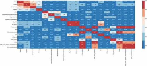
After mutual information, Pearson’s correlation feature selection technique was utilized to find redundant features. This feature selection technique compares the degree of association among all variables (Okunev, 2022). When there is a high correlation between two independent attributes, one of these attributes can be removed since both features contribute the same to the ML model. This method can also be applied to determine if the independent and target variables have a positive or negative correlation. The Pearson correlation coefficient “r” determines the extent of association between variables. The r values lie between −1 and 1. A positive correlation is shown when the r value is close to 1, and a negative correlation is shown when the r value is close to −1. This methodology is founded on the notion that by assessing the strength of the relationship between different clinical parameters, it is possible to determine the relevance of a significant attribute in the dataset. A Pearson’s correlation heat map is described in Figure 8. It can be observed that among all variables, the “Schiller’s test” and the “Hinselmann’s test” positively correlate with the biopsy result. The cytology test also plays an important role in the diagnosis. From the figure, it can be observed that combining the results obtained by the above tests along with machine learning can be highly influential in predicting the biopsy results. Further, it can be observed that the attributes “STDs”, “STDs_vulvo_perineal_condylomatosis” and “STDs_condylomatosis” have a high correlation among themselves. Hence the attributes “STDs_vulvo_perineal_condylomatosis” and “STDs_condylomatosis” were removed from the dataset. A high correlation also exists between “STDs_number” and “STDs_No_of_diagnosis”. Hence, “STDs_No_of_diagnosis” attribute was removed. After using the above three feature selection methods, 15 attributes were chosen for training the classifiers.

Figure 8. Pearson’s correlation heatmap which describes the relationship among various attributes which diagnose cervical cancer.

3.4. Oversampling using borderline-SMOTE

Many medical datasets suffer from data imbalances, which skews the model output (DC Li et al., 2010). Generally, there are three levels of imbalance: mild, moderate and extreme. The imbalance is problematic since the classifiers prioritize the majority class. Generally, there are two approaches to fix this issue. Under-sampling and oversampling. Under-sampling involves minimizing or reducing the major class size to equal the minor class. Oversampling involves utilizing a specific algorithm to add new samples to the minor class. Oversampling is favoured since it prevents the loss of essential data and intriguing patterns.

SMOTE outperforms the conventional oversampling approach (Maldonado et al., 2022). The latter replicates the minority class group. As a result, the dataset automatically grows. Since the dataset is created using mere duplication, no new variations or patterns will be obtained, which might be helpful to the classifiers. When the dataset is small, this can also lead to overfitting. The k-nearest neighbours’ classifier is used in SMOTE to generate synthetic data (Maldonado et al., 2022). Starting with random data from the minority occurrences, SMOTE chooses the best k-nearest neighbours. Further, new data is created between the neighbours and instances. This procedure is repeated until the fraction of the two categories is equal. However, there is a problem with this algorithm. If data exists in the minor class that is aberrant and appear in the major class, it establishes a line bridge with the majority class. This reduces the efficiency of the oversampling technique. A variant of SMOTE, the Borderline-SMOTE, resolves this problem (K Li et al., 2022). In Borderline-SMOTE, the data points present in the minority class are initially classified. When generating synthetic data, data points are considered noise if all the data’s neighbours belong to the major class. A few observations with neighbours from the major and minor classes are individually sub-sampled. To balance the cervical cancer data, the Borderline-SMOTE technique was utilized. Figure 9 compares the size of the two classes before and after balancing the data. In Figure 9b, it can be observed that there are equal instances of positive and negative biopsy results.

Figure 9. Biopsy results before and after balancing. (a) Initial unbalanced data (b) Balanced data after using Borderline-SMOTE.

4. Results and discussion

The heterogeneous ML classifiers are tested and evaluated in this section. Further, explainable AI techniques such as SHAP, LIME and random forest are utilized to understand the most helpful parameters. In the last sub-section, various parameters are discussed from a medical perspective. In Figure 10, this research’s process flow is depicted. In the beginning, the dataset of patients who got tested for cervical cancer was analyzed and pre-processed. Three feature selection methods: ANOVA, mutual information and Pearson’s correlation was used and the number of features was narrowed down to fifteen. Since imbalanced data does give reliable results, Borderline-SMOTE technique was used to balance the positive and negative biopsy results. Then the custom stacking architecture of ML models was used to train and test the classifier. The stacking consisted of multiple levels to ensure heterogeneity and reliability. The final stacking model was used for prediction. A user interface system was built using the “Gradio” library. This user interface can be deployed in real time to verify the results and to give a second opinion to the doctors.

Figure 10. Various steps followed to predict biopsy results using machine learning.

4.1. Model evaluation

In this research, a custom stacked ensemble model has been used to predict the biopsy results of cervical cancer patients. These models can confirm the results of the biopsy test, and if there is a disparity, the patient can undergo the biopsy test again. The false negative results can be easily avoided by deploying these classifiers in real-time. To improve the performance metrics, several ML models have been utilized and then combined on various levels using a stacked model. Figure 11 describes the entire model architecture. In the beginning, five routine ML models such as logistic regression and decision tree were trained and tested individually. Further, these models were combined to form the first stacked model named “STACKA”. Seven bagging, boosting and multi-layer perceptron models were tested parallelly to predict the biopsy results. These models were combined further to form the second stacked model named “STACKB”. To achieve optimal results, “STACKA” and “STACKB” were combined to form “STACKC”. This multi-layer stacked model was used for final prediction.

Figure 11. Custom stacking architecture to predict cervical cancer biopsy results.

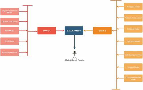
All the models were hyperparameter tuned using the grid search technique. Initially, ML models in medical AI were utilized, including logistic regression, KNN, Naïve Bayes, decision tree and support vector machine. To increase the efficiency of the model, they were ensembled using the stacking class (Kim et al., 2021). Besides performance, stacking models are more reliable since the results obtained by them are based on many models. Stacking combines the algorithms using a “voting-strategy” and improves the predictive performance. It understands how to integrate different predictions by employing a meta-learning technique. The significant advantage of this algorithm is that it can combine the strengths of numerous precise classifiers to provide predictions which outperform any individual model. The stacked model was named “STACKA”. As a consequence, the proportion of patients who tested positive and negative in the biopsy test were equal in number. To increase performance and avoid overfitting, the train and test data were randomly shuffled using a 5-fold cross validation approach. Further, bagging and boosting algorithms were used for prediction. They are more advanced than the traditional classifiers. These include adaptive boosting (adaboost), random forest, categorical boosting (catboost), light gradient boosting machine (light gbm), multi-layer perceptron, xgboost and extra trees classifier. The second stacked model, known as “STACK B”, was created by combining the above models. Further, “STACKA” and “STACKB” were combined to form “STACKC”. This optimized model was used to predict the cervical cancer biopsy results. To understand the impact of Borderline-SMOTE, the models were tested without data balancing in the beginning. Table 4 describes the results of the classifiers without using feature selection and Borderline-SMOTE method. The final “STACKC” model was able to obtain an accuracy of 74%. The precision, recall and f1-score obtained were 50%, 60% and 55% respectively.

Table

Algorithm 1. Feature selection using ANOVA.
Input:	M: Size Sn * H feature matrix; where Sn-number of samples, H- number of features
Output:	Best N Marchkers
1:	Read the dataset, Replace the missing values.
2:	For every gi in the feature set do
3:	j = 1,2,3, … .H
4:	The value of MS can be calculated by equation (3)(3) $MS=SE/DF$(3)
5:	Calculate MSL using equation (6)(6) $MSL=ICR/DFC$(6)
6:	Find the value of F-statistic (F) by equation (7)(7) $F=MS/MSL\hspace{0.17em}$(7)
7:	Use the F-distribution table and calculate the p-value(pj) for all F-statistics
8:	If pj < 0.001 then
9:	Choose feature gj
10:	Concatenate gj to feature matrix Hm
11:	Else
12:	Feature gj is removed
13:	End if
14:	Using p value, arrange all the features based on their importance
15:	If feature_size (Hm) > 18 then
16:	Only choose the best 18 Marchkers
17:	Else
18:	Keep all the Marchkers in Hm
19:	End if
20:	End for
21:	Return Hm

Table 4. Performance evaluation of classifiers without using feature selection and borderline-SMOTE (Unbalanced dataset)

Classifier	Accuracy (%)	Precision (%)	Recall (%)	F1-score (%)
Logistic regression	78	59	67	62
Decision tree	47	0	0	0
K Nearest Neighors	75	53	53	53
Support vector machine	78	57	87	68
Naïve Bayes	62	24	93	38
STACKA (Logistic regression + Decision tree + K Nearest Neighbors + support vector machine + Naïve Bayes)	75	53	67	59
Random forest	79	60	60	60
Multi-layer perceptron	62	24	93	38
Adaboost	79	58	93	72
Catboost	74	50	67	57
Lightgbm	72	55	80	65
Xgboost	77	55	80	65
Extra trees	47	0	0	0
StackB (Random forest + Multi-layer perceptron + Adaboost + Catboost + Lightgbm + xgboost + Extratrees)	74	50	60	55
STACKC (STACKA + STACK B)	74	50	60	55

Logistic regression is the method of estimating the likelihood of a discrete outcome when many input attributes are provided (Dumitrescu et al., 2022). When the two classes are linearly separable, the algorithm works efficiently. All the values are converted between “0” and “1” using the sigmoid function. For the cervical cancer dataset, the accuracy, precision, recall, F1-score, AUC and average precision (AP) obtained by the logistic regression model were 95%, 95%, 95%, 95%, 98% and 96% respectively. A decision tree uses a tree like structure to classify instances (Fryan et al., 2022). The labels are represented by a leaf node, a tree-branch determines an outcome and all attributes are present as internal nodes. The best splitting attribute becomes the root node. Subdividing the source data into smaller chunks is the foundation of the “learning” process in decision tree. This process is also called “recursive portioning”. This phase concludes when a node’s subgroup contains the exact dependent label or when further splits do not increase the performance. The model can be constructed without a domain expert, making it ideal for investigative information retrieval. Generally, tree-based classifiers are capable of handling high-dimensional data with ease. For the cervical cancer dataset, the accuracy, precision, recall, f1-score, AUC and AP obtained were 97%, 97%, 97%, 97%, 98% and 97% respectively.

KNN uses a non-parametric algorithm to classify instances (Salem et al., 2022; S Zhang et al., 2022). It is also well known for consistently classifying non-linear datasets. It is founded on the idea of grouping entities in a certain feature space based on comparable observations. When the model acquires new datapoints, it determines the class of the updated data by looking at the category of the k nearest data points. Analysis involves evaluating how factors such as classification guidelines and distance metrics affect results. It is a simple algorithm and is fairly effective in most cases. However, the presence of noisy data, outliers and data imbalance might hinder the performance of the model. In this research, the dataset has been systematically preprocessed to eliminate noise and outliers. The KNN was able to obtain an accuracy, precision, recall, f1-score, AUC and AP of 98%, 98%, 99%, 98%, 98% and 97%. Finding the ideal support vectors to classify the data using a n-dimensional space is the principle of the support vector machine (SVM) classifier (Dinesh & Kalyanasundaram, 2022). The closest data elements for the two categories are intersected by two Marginal lines that run parallel to the bounding hyper plane. These points are referred to as support vectors. To improve performance, the classifier seeks to widen the Marginal distance. Various types of kernels are used such as linear, radial basis function (rbf), sigmoid and others. For the cervical cancer dataset, the linear kernel obtained the maximum accuracy. The accuracy, precision, recall, f1-score, AUC and AP obtained were 96%, 96%, 96%, 96%, 97% and 94% respectively. Naïve Baye’s classifier uses the “Bayes theorem” of conditional probability to classify the instances (Khanna & Sharma, 2018). It is founded on the notion that each pair of features being categorized are unique. Further, the entire data is split into two parts: feature matrix and response vector. For the cervical cancer data, the accuracy, precision, recall, f1-score, AUC and AP obtained were 94%, 92%, 97%, 95%, 98% and 97%, respectively.

All the above classifiers were combined together using the stacking methodology to form “STACKA”. Several regression and classification models can be custom-ensembled using stacking. The most commonly used ensemble methods are bagging and boosting. To lower entropy, bagging permits the averaging of numerous classifiers with higher variance. Boosting develops several incremental techniques to minimize bias and variance. The stacking methodology takes a difference approach. The idea entails in addressing a learning problem using a number of models. It is possible to construct multiple unique learners in order to produce an intermediate prediction. Following that, a new classifier is added that uses the prediction from the previous intermediate classifiers. As implied by the name, the final classifier is stacked using different classifiers. This increases performance and frequently outperforms individual models. Since they were created using several heterogenous classifiers, the results are also more reliable. The accuracy, precision, recall, f1-score, AUC and AP obtained by the “STACKA” model are 98%, 98%, 98%, 98%, 100% and 100%. The results are described in Table 5. The ROC curves and the precision recall curves are described in Figures 12 and 13, respectively. From Figure 12, it can be observed that “STACKA” obtained the highest accuracy.

Figure 12. ROC curves obtained by the classifiers. (a) Logistic regression (b) Decision tree (c) KNN (d) SVM (e) Naïve Bayes (f) STACK A.

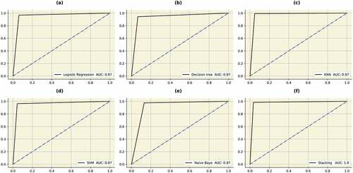
Figure 13. Precision-recall curves of the initial set of classifiers.

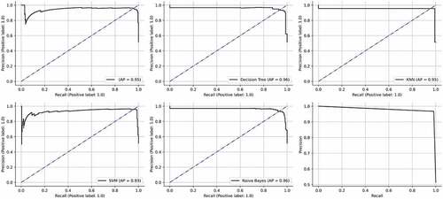
Table 5. Performance evaluation of the initial set of classifiers after data balancing and hyperparameter tuning

Classifier	Accuracy (%)	Precision (%)	Recall (%)	F1-score (%)	AUC (%)	AP (%)	Best hyperparameters
Logistic regression	95	95	95	95	98	96	{“C”: 1, “penalty”: “l2”}
Decision Tree	97	97	97	97	98	97	{“criterion”: “entropy”, “max_depth”: 8, “max_features”: “log2”, “min_samples_leaf”: 1, “min_samples_split”: 10, “splitter”: “best”}
KNN	98	98	99	98	98	97	{“n_neighbors”: 1}
Support vector machine	96	96	96	96	97	94	{“kernel”:’linear’, “probability”:’True’}
Naïve Bayes	94	92	97	95	98	97	-
STACKA (Logistic regression + Decision tree + K Nearest Neighbors + support vector machine + Naïve Bayes)	98	98	98	98	100	100	{“Meta classifier”:’logistic regression’}

After evaluating initial models, classifiers which used bagging and boosting methodology were trained and tested. Random forest is a popular algorithm which can be used for classification as well as regression (MZ Alam et al., 2019). It is very flexible, accurate and simple. It can also be adjusted for different datasets. Due to the fact that it combines numerous decision trees, the term “forest” is used. The trees autonomously make decisions, which are subsequently combined to provide to provide high-quality outcomes. The model is also made more unpredictable by choosing the best attribute at random from an initial set of features. Each decision tree can produce a different set off results using a technique called bagging (bootstrap aggregation). Only a portion of data is used by each tree. Each individual tree takes decision based solely on the data it has access to and makes predictions. This ensures that the trees are trained using various parts of the dataset. Therefore, the inaccurate predictions and entropies are significantly decreased. Over-fitting caused by the decision trees can be easily prevented using this method. The random forest was able to obtain an accuracy, precision, recall, f1-score, AUC and AP of 96%, 96%, 97%, 96%, 99% and 100%, respectively. Multi-layer perceptron uses the” neural network” to classify instances (Hosseinzadeh et al., 2021). It uses the methodology of forward and backward propagation to optimize the loss function. Each attribute is assigned a weight. The sum of the weighted attributes and bias is sent to the different layers of the neural network using an activation function. Afterwards, the neural network makes a decision. The loss function is used to find the difference between the actual and predicted values. During the back propagation, the weights are updated using an optimizer. The function of the neural network is to minimize the loss function by continuously updating the weights. The MLP model was able to obtain an accuracy of 94%, 92%, 96%, 94%, 97% and 96%. After hyperparameter tuning, the best optimizer was “Adam” and the activation function used was “tanh”. A constant learning rate was adapted and the neural network was trained for thirty iterations. Adaboost utilizes the concept of “weak learners” to make accurate predictions using a series of decision trees (Hatwell et al., 2020). The weights of the inaccurate results are increased after each iteration. With the exception of the trees in the first iteration, which is created during training, all trees are descended from the previous iterations. After the creation of initial trees, inaccurate records are prioritized. The newly created trees then receive these instances that were incorrectly labelled. The process is repeated until the number of base learners exceed a certain limit. The adaboost was able to obtain an accuracy, precision, recall, f1-score, AUC and AP of 98%, 97%, 98%, 98%, 99% and 99%. Extreme gradient boosting (xgboost) is derived from the gradient boosting architecture (Li & Zhang, 2020). It uses the “gradient descent” methodology to decrease the loss function. The algorithm can be easily parallelized too. “Tree pruning” is used to control the depth of the tree. It uses L1 (Lasso) and L2 (Ridge) regularization to prevent model overfitting. In this research, the xgboost algorithm was able to obtain an accuracy, precision, recall, f1-score, AUC and AP of 98%, 96%, 100%, 98%, 99% and 100%. Categorical boosting (catboost) is highly beneficial when there are a lot of categorical input features (Hancock & Khoshgoftaar, 2020). In this model, the features are ordered using a concept called “target statistics” (For each category, a target value is estimated). The catboost algorithm was able to obtain an accuracy, precision, recall, f1-score, AUC and AP of 97%, 96%, 99%, 98%, 99% and 99%, respectively. The light gradient boosting machine (lightgbm) minimizes memory usage during classification (Zhang & Gong, 2020). The model utilizes two novel techniques to eliminate histogram-based classification. These are gradient based one-side sampling (GOS’s) and exclusive feature bundling (EFB). Together, they enable the model to function efficiently and provide it a significant edge over other boosting classifiers. The lightgbm obtained an accuracy, precision, recall, f1-score, AUC and AP of 98%, 97%, 98%, 98%, 100% and 100%. In extra trees classifier, various de-correlated trees are combined to improve the performance the model (Gupta et al., 2022). With its exception of its architecture, it is comparable to the random forest model. This classifier obtained an accuracy, precision, recall, f1-score, AUC and AP of 94%, 96%, 93%, 95%, 98% and 97%, respectively. All the bagging and boosting algorithms were further combined to form “STACKB” model using logistic regression as meta-classifier. The “STACKB” model was able to obtain an accuracy, precision, recall, f1-score, AUC and AP of 98%, 98%, 98%, 98%, 100% and 100%, respectively. “STACKA” and “STACKB” were further combined to form “STACKC” model. This final multi-level ensembled model obtained an accuracy, precision, recall, f1-score, AUC and AP of 98%, 97%, 99%, 98%, 100% and 100%. For predicting the cervical cancer biopsy results, the “STACKC” model would be used. The results are sumMarchized in Table 6. The ROC curve and precision-recall curves of the algorithms are described in Figures 14 and 15. The confusion matrices for “STACKA”, “STACKB” and “STACKC” are described in Figure 16. From the figure it can be observed that the number of false positive and false negative cases are very few which contributes to high accuracy

Figure 14. AUC’s of the bagging, boosting and stacking classifiers. (a) Random forest (b) MLP (c) Adaboost (d) Catboost (e) Lightgbm (f) Xgboost (g) Extratrees (h)STACKB (i) STACKC.

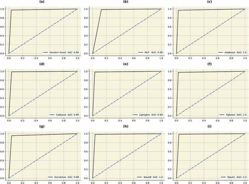
Figure 15. Precision-recall curves of the bagging, boosting and stacking classifiers.

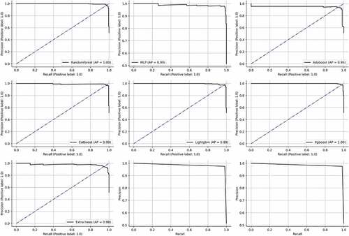
Figure 16. Confusion matrices: (a) STACK A (b) STACK B (c) STACK C.

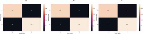
Table 6. Performance evaluation of bagging and boosting classifiers after data balancing and hyperparameter tuning

Classifier	Accuracy (%)	Precision (%)	Recall (%)	F1-score (%)	AUC (%)	AP (%)	Best hyperparameters
Random forest	96	96	97	96	99	100	{“bootstrap”: True, “max_depth”: 100, “max_features”: 2, “min_samples_leaf”: 3, “min_samples_split”: 8, “n_estimators”: 200}
Multi-layer perceptron	94	92	96	94	97	96	{“activation”: “relu”, “alpha”: 0.05, “hidden_layer_sizes”: (100,), “learning_rate”: “constant”, “max_iter”: 50, “solver”: “lbfgs”}
Adaboost	98	97	98	98	99	99	{“learning_rate”: 1.0, “n_estimators”: 300}
Catboost	97	96	99	98	99	99	{“border_count”: 10, “depth”: 3, “iterations”: 250, “l2_leaf_reg”: 1, “learning_rate”: 0.03}
Lightgbm	98	97	98	98	99	99	-
Xgboost	98	96	100	98	99	100
Extratrees	94	96	93	95	98	97
STACK B ((Random forest + Multi-layer perceptron + Adaboost + Catboost + Lightgbm + xgboost + Extratrees)	98	98	98	98	100	100	{“Meta classifier”:’logistic regression’}
STACK C (STACKA +STACKB)	98	97	99	98	100	100	{“Meta classifier”:’logistic regression’}

Multiple ML models were employed as a part of a retrospective evaluation study to predict the diagnosis in cervical cancer patients. This study focuses on the development, validation and application of multiple classifiers to quickly identify patients who are at a risk of getting diagnosed with cancer.

4.2. Interpreting results with explainable AI

The people may now comprehend and trust the results produced by machine learning algorithms owing to a combination of techniques and processes known as Explainable Artificial Intelligence (Tjoa & Guan, 2020). Along with a thorough understanding of the model output, the classifier’s biases and impacts can also be understood using this technique. It helps define the algorithm’s accuracy, transparency, correctness and effectiveness in decision making. Since AI is evolving at a rapid pace, it is crucial for people to comprehend the results obtained by the ML models. The entire calculation process is converted into a “black box”, which is more difficult to understand. However, Explainable AI can easily decipher this issue. There are numerous benefits of interpreting a classifier. The results obtained by the model become easier to understand. It also improves the trustworthiness and reliability of the ML model. Additionally, it aids researchers from various back ground in understanding the predictions made by the classifiers. There are four Explainable AI techniques used in this research: SHAP, LIME, random forest and ELI5.

The fate of the individuals will be greatly impacted by cutting-edge decisions made in medical settings employing AI, despite the many legal and ethical ramifications. As a result, there is a great need for reliable and understandable classifiers. The healthcare practitioners should have the capability to comprehend the result and predictions. They should be able to make reliable conclusions after understanding the predictions of the ML model. To maintain the robustness and predictability of the model, feature importance using Explainable AI is essential. To determine how each feature impacts the biopsy result, SHAP compares the anticipated value with the prediction using Shapley values (Y Liu et al., 2022). Figure 17a describes a bee swarm plot which analyzes both positive and negative biopsy result predictions. This plot displays Shapley values and incorporates the significance of each attribute from all the relevant features. On the left, the attributes are arranged in the descending order of their importance. The color blue represents a lower value and the color red represents a higher value. According to SHAP, the “Schiller’s test” is the most important attribute. A positive Schiller’s test result most likely indicates a positive biopsy result. Other features which are important are Hinselmann’s test, citology test, the number of pregnancies, the number of STD’s, the number of years a contraceptive has been used, patient age and others. From the figure it can also be inferred that the risk of contracting cervical cancer increases if the patients had many pregnancies. The presence of other STD’s can also lead to cervical cancer. Older patients are also more vulnerable to get diagnosed with a positive biopsy result. The most significant features are determined using the attribute mean, as described in Figure 17b. Schiller’s test, Hinselmann’s test, Citology test, the number of pregnancies, the number of STDs and the usage of hormonal contraceptives (in years) are critical factors.

Figure 17. Feature importance using SHAP. (a) Bee swarm plot (b) Mean SHAP values.

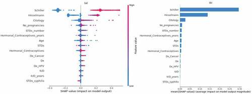
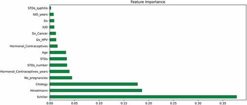
In random forest feature importance, each projected value is randomly shuffled and the model determines the importance of each feature by monitoring the impact on the accuracy of the model (X Li et al., 2019). Figure 18 presents the importance of each feature in ascending order of their importance. The most important features are the Schiller’s test, Hinselmann’s test, citology test, the number of pregnancies and the use of contraceptives (in years). It verifies and supports the most important indicators discovered through SHAP analysis.

Figure 18. Feature importance using random forest.

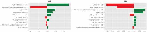
LIME is classifier independent and can be used with any ML model. This approach seeks to evaluate the model by altering the data points and monitoring how the predictors change (Islam et al., 2022). Specific techniques try to understand the black box model by looking at its dynamics. Additionally, it modifies the feature value and monitors the impact on the output. It also offers a list of justifications highlighting the importance of each attribute in relation to the prediction. This provides reliable inference and enables the identification of feature changes which improve prediction quality. Figures 19 and 20 describes the feature importance using LIME model for a positive and negative biopsy result. The color orange indicates a positive result and the color blue indicates a negative result. Unlike SHAP, feature importance using LIME can be interpreted for each patient. In Figure 19, LIME explains a positive biopsy result. Various attributes such as the Schiller’s test, Hormonal contraceptives used (in years), the number of pregnancies, patient age and the Hinselmann’s test all indicate a positive diagnosis. The probabilities of all the features are considered into account. In Figure 20, LIME interprets a negative biopsy result. The attributes syphilis and the Schiller’s test play a crucial factor to the ML model in making this prediction. Even though some features indicate a positive diagnosis, the model still predicts a negative diagnosis since the above two parameters have been assigned more weights by the classifier. Figure 21a and b represents the LIME interpretation using bar graphs for a cancerous and non-cancerous patient, respectively. The planes are divided by a vertical line. The left side of the hyperplane represents a positive biopsy result and the right side of the hyperplane represents a negative biopsy result. In Figure 21a, attributes such as the Schiller’s test, age, syphilis and the number of STD’s indicate a positive cervical cancer diagnosis. In Figure 21b, attributes such as the Schiller’s test, syphilis and the number of STD’s indicate a negative diagnosis. After using three feature importance techniques, it can be inferred that the Schiller’s test is the most important attribute to predict biopsy results. The decision-making process for doctors and other physicians becomes easy by using Explainable AI techniques. Additionally, the findings are simple to interpret and convey to others.

Figure 19. Feature importance using LIME (Positive Biopsy result).

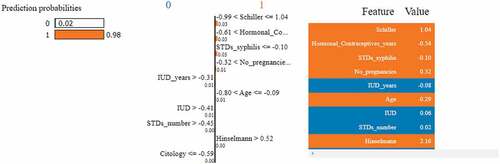
Figure 20. Feature importance using LIME (Negative Biopsy result).

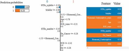
Figure 21. Feature importance using LIME graphs. (a) Positive biopsy result (b) negative biopsy result.

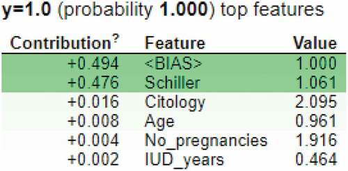
ELI5 is an explainable AI technique which interprets the predictions of a ML classifier (Islam et al., 2022). It can be used by classifiers and regressors. It works for various frameworks and packages such as scikit-learn, keras, xgboost, catboost, lightining, sklearn-crfsuite and many more. In this research, ELI5 was used to understand the predictions made by the decision tree model. Figure 22 shows the contribution values of various features in predicting the cervical cancer positive result. According to this feature importance technique, the most important features are: “Schiller’s test”, ”Citology test”, “Age”, “Number of pregnancies” and the number of years an IUD has been used. The ELIF algorithm considers “bias” to explain the model predictions too.

Figure 22. Feature importance using ELI5 for cervical cancer positive biopsy result.

4.3. Discussion

In this research, machine learning is used to examine a set of clinical parameters which could possibly predict cervical cancer. The change in these parameters can be crucial to identifying this deadly disease. Various tests such as the Schiller’s test, cytology test, Hinselmann’s test and the biopsy test are used to come to a final diagnosis. According to the study, the Schiller’s test is the most important in predicting the biopsy results. In this test, iodine solution is applied to the cervical tissues. The color of the healthy cells changes to brown and the color of the abnormal cells do not change (Jaya & Latha, 2022). This iodine solution is also known as the Lugol’s solution. The cytology test is also very important in cervical cancer diagnosis (da Silva et al., 2022). This method is used to identify pre-invasive cervical lesions (high grade cervical intraepithelial neo plasma) at a preliminary stage. It is a process in which tissues are removed from the surface of the cervix. The examination of these tissues is done under a microscope to find all alterations which may result in cervical cancer. The Hinselmann’s test is a technique to accurately examine the cervix for signs of infection and diseases. During the test, a special instrument called the colposcope is utilized (Yoon et al., 2022). Studies have shown that taking oral contraceptives over a period of time increases the risk of contracting cervical cancer (La Vecchia & Boccia, 2014). Our research agrees with the same and women using hormonal contraceptives for a long period of time had tested positive for the biopsy result. According to studies, women between the ages of 36 and 45 are most susceptible to this disease (Bruni et al., 2022). Our studies agree with the same. Cervical cancer can also be caused by other STD’s such as syphilis, herpes, chlamydia and gonorrhea (Pillai et al., 2022). Generally, cervical cancer is associated with HPV virus, but it can also be caused by other viruses. The usage of IUD’s decreases the chance of contracting cervical cancer according to many researches (Averbach et al., 2018). The results obtained by the models agree with the above concept. IUD use lowers the risk of contracting adenosquamous carcinoma and squamous cell carcinoma, the two main kinds of cervical cancer. During the initial year of IUD use, the likelihood for both malignancies was found to be lowered by almost half. Figure 23 describes the user interface built to make biopsy result predictions. The final stacked model was deployed using the “gradio” library (Abid et al., 2019). There are various textboxes which can be filled with attribute values. Once the submit button is pressed, the prediction is made in the output text box. The model can be deployed in various hospitals as a preliminary screening tool.

Figure 23. User interface of the prediction model deployed using “Gradio” to classify cervical cancer results.

Various researchers have used multiple ML models to diagnose cervical cancer. Yang et al. (W Yang et al., 2019) used multiple classifiers to diagnose cervical cancer. For the biopsy result, a maximum accuracy of 96.2% was obtained. Akter et al. (Akter et al., 2021) used ML techniques to predict cervical cancer from behavioral risk features. A maximum accuracy of 93.33% was obtained. Deng et al. (Deng et al., 2018) obtained an accuracy of 97% using random forest for the similar dataset used in our study. According to the study, random forest performs better than xgboost and support vector machine. The rest of the researches along with our study is described in Table 7.

Table 7. Comparison of various researches

Reference	Year	Models used	Number of Classes	Accuracy (%)	Precision (%)	Recall (%)	F1-score (%)	AUC (%)
(Chauhan & Singh, 2022)	2022	Various ML models	2	98	98	100	97	99
(Curia, 2021)	2021	Various ML models	2	94.5	-	-	-	98
(Jahan et al., 2021)	2021	Various ML models	2	96	95	96	95	-
(Nithya & Ilango, 2019)	2019	Various ML models	2	100	-	-	-	91
(Fernandes, Chicco, et al., 2018)	2018	Various ML models	2	98	98	98	98	96
[42	2022	Various ML models	2	97	-	-	-	-
(Aloss et al., 2022)	2022	Various ML models	2	97	-	-	-	-
(Tanimu et al., 2022)	2022	Various ML models	2	98	-	-	-	-
(Nsugbe, 2022)	2022	Various ML models	2	91.5	-	96	-	95
(Nagadeepa et al., 2022)	2022	Various ML models	2	97%	-	-	-	-
Proposed study	-	Custom multi-layer Stacking models	2	98	97	99	98	100

Machine learning and Artificial intelligence help various biomedical systems in automating the diagnosis of various diseases (Al-Issa & Alqudah, 2022; Alqudah & Alqudah, 2022b, 2021b). A lot time can be reduced if the ML algorithms deliver results with high accuracy (Chen et al., 2022; Rahaman et al., 2020). It can ease the burden on healthcare workers. It can also be used by doctors to get a second opinion regarding the prognosis and treatments (W Liu et al., 2022; J Zhang et al., 2021). The patient data can be analyzed and preprocessed extensively. This can result in getting to understand various hidden and exciting patterns (Rahaman et al., 2021). They can also be used for bench Marchking. Health informatics is a trending topic in today’s world (Chadaga et al., 2022). The use of AI, ML and data science can help us gain valuable insights about the data (Al-Issa et al., 2022; Alqudah, Al-Hashem, et al., 2021). Various deadly diseases such as COVID-19 and monkey pox have emerged in the past two years. Hence, it is vital to use emerging technologies to tackle these diseases (Chadaga et al., 2021; Pradhan et al., 2022; Sharma & Mishra, 2022, 2021). Machine learning and Artificial Intelligence can be a silver lining for the current and future generations in aiding the healthcare sector.

5. Conclusion

According to WHO, 80% of cervical cancer cases are diagnosed in developing nations. If not detected at an early stage, this cancer can be fatal. This research uses a custom stacked ensemble model to predict the biopsy results using various clinical parameters. Before training the models, feature selection methods such as ANOVA and Pearson’s correlation have been utilized to identify important parameters. Since the dataset was unbalanced, Borderline-SMOTE was used for data balancing. Afterwards, various models were trained and tested for cervical cancer classification. Further, the algorithms were combined on various levels to form the final stacked model. This classifier obtained an accuracy, precision, recall, f1-score, AUC and AP of 98%, 97%, 99%, 98%, 100% and 100%. To achieve better interpretability, explainable AI was used. SHAP, LIME and random forest were used to understand the model predictions. Among all the parameters, the “Schiller’s test result” was the most important. A user interface application was built using the “Gradio” library, which can be deployed in real-time to assist medical professionals.

However, various issues must be addressed before deploying the classifiers in health care facilities. Rigorous testing must be conducted, followed by thorough external validation. The datasets should be of high quality too. Bridging the knowledge gap between medical and ML professionals is also extremely crucial.

Availability of data and materials

Data and materials will be made available if sincere request is made to the corresponding author.

Disclosure statement

No potential conflict of interest was reported by the author(s).

Additional information

Funding

Open access funding will be provided by Manipal Academy of Higher Education, Manipal.

Notes on contributors

Krishnaraj Chadaga

Krishnaraj Chadaga is currently pursuing Ph.D in Manipal Institute of Technology (Institute of Eminence), Manipal, India. His research interests lie in Medical Artificial Intelligence and Health Informatics. Dr. Srikanth Prabhu is an Associate Professor (Senior Scale) in the Department of Computer Science and Engineering, Manipal Institute of Technology. His research interests are forensics and machine learning. Dr. Niranjana Sampathila is an Associate Professor (Senior Scale) in the Department of Biomedical Engineering. His current research interest is Explainable Artificial Intelligence for Health care domain. Mr. Rajagopala Chadaga is an Associate Professor (Senior Scale) in the Department of Mechanical and Manufacturing Engineering. He is proficient in machine learning techniques. Dr. Swathi KS is an Assistant professor in Manipal Institute of Technology. Her expertise lies in healthcare management. Dr. Saptarshi Sengupta is an Assistant Professor in San Jose State University, United States of America. His research interests are swarm intelligence and fuzzy logic

References

- Abid, A., Abdalla, A., Abid, A., Khan, D., Alfozan, A., & Zou, J. (2019). Gradio: Hassle-free sharing and testing of ml models in the wild. https://doi.org/10.48550/arXiv.1906.02569
- Akter, L., Islam, M., Al-Rakhami, M. S., & Haque, M. (2021, May). Prediction of cervical cancer from behavior risk using machine learning techniques. SN Computer Science, 2(3), 1. https://doi.org/10.1007/s42979-021-00551-6
- Alam, Z., Dean, J., & Janda, M. (2022, April). What do South Asian immigrant women know about HPV, cervical cancer and its early detection: A cross-sectional Australian study. Journal of Migration and Health, 8, 100102. https://doi.org/10.1016/j.jmh.2022.100102
- Alam, M. Z., Rahman, M. S., & Rahman, M. S. (2019, January 1). A random forest based predictor for medical data classification using feature ranking. Informatics in Medicine Unlocked, 15, 100180. https://doi.org/10.1016/j.imu.2019.100180
- Al-Hashem, M. A. (2021). Performance evaluation of different machine learning classification algorithms for disease diagnosis. Ijehmc, 12(6), 1–38. http://doi.org/10.4018/IJEHMC.20211101.oa5
- Al-Issa, Y., & Alqudah, A. M. (2022). A lightweight hybrid deep learning system for cardiac valvular disease classification. Scientific Reports, 12(1), 1–20. https://doi.org/10.1038/s41598-022-18293-7
- Al-Issa, Y., Alqudah, A. M., Alquran, H., & Al Issa, A. (2022). Pulmonary diseases decision support system using deep learning approach. Computers, Materials & Continua, 73(1), 311–326. https://doi.org/10.32604/cmc.2022.025750
- Aloss, A., Sahu, B., Deeb, H., & Mishra, D. (2022). A crow search algorithm-based machine learning model for heart disease and cervical cancer diagnosis. In InElectronic systems and intelligent computing (pp. 303–311). Springer. https://doi.org/10.1007/978-981-16-9488-2_27
- Alqudah, A. M., Al-Hashem, M., & Alqudah, A. (2021). Reduced number of parameters for predicting post-stroke activities of daily living using machine learning algorithms on initiating rehabilitation. Informatica, 45 (4).
- Alqudah, A., & Alqudah, A. M. (2021a, May). Sliding window based deep ensemble system for breast cancer classification. Journal of Medical Engineering & Technology, 45(4), 313–323. https://doi.org/10.1080/03091902.2021.1896814
- Alqudah, A., & Alqudah, A. M. (2021b, September). Artificial intelligence hybrid system for enhancing retinal diseases classification using automated deep features extracted from OCT images. International Journal of Intelligent Systems and Applications in Engineering, 9(3), 91–100. https://doi.org/10.18201/ijisae.2021.236
- Alqudah, A. M., & Alqudah, A. (2022a, February). Deep learning for single-lead ECG beat arrhythmia-type detection using novel iris spectrogram representation. Soft Computing, 26(3), 1123–1139. https://doi.org/10.1007/s00500-021-06555-x
- Alqudah, A. M., & Alqudah, A. (2022b). Improving machine learning recognition of colorectal cancer using 3D GLCM applied to different color spaces. Multimedia Tools and Applications, 81(8), 10839–10860. https://doi.org/10.1007/s11042-022-11946-9
- Alqudah, A., Alqudah, A. M., Alquran, H., Al-Zoubi, H. R., Al-Qodah, M., & Al-Khassaweneh, M. A. (2021). Recognition of handwritten Arabic and hindi numerals using convolutional neural networks. Applied Sciences, 11(4), 1573. https://doi.org/10.3390/app11041573
- Alqudah, A. M., Qazan, S., & Masad, I. S. (2021). Artificial intelligence framework for efficient detection and classification of pneumonia using chest radiography images. Journal of Medical and Biological Engineering, 41(5), 599–609.
- Alquran, H. et al. (2022). Cervical cancer classification using combined machine learning and deep learning approach. Comput. Mater. Contin, 72(3), 5117–5134.
- Alsharif, R., Al-Issa, Y., Mohammad Alqudah, A., Abu Qasmieh, I., Azani Mustafa, W., & Alquran, H. (2021). PneumoniaNet: Automated detection and classification of pediatric pneumonia using chest X-ray images and CNN approach. Electronics, 10(23), 2949. https://doi.org/10.3390/electronics10232949
- Arbyn, M., Castle, P. E., Schiffman, M., Wentzensen, N., Heckman‐Stoddard, B., & Sahasrabuddhe, V. V. (2022). Meta-analysis of agreement/concordance statistics in studies comparing self- vs clinician-collected samples for HPV testing in cervical cancer screening. International Journal of Cancer, 151(2), 308–312. https://doi.org/10.1002/ijc.33967
- Averbach, S., Silverberg, M. J., Leyden, W., Smith-McCune, K., Raine-Bennett, T., & Sawaya, G. F. (2018). Recent intrauterine device use and the risk of precancerous cervical lesions and cervical cancer. Contraception, 98(2), 130–134. https://doi.org/10.1016/j.contraception.2018.04.008
- Beer, T. M. (2021, December). Examining developments in multicancer early detection: Highlights of new clinical data from recent conferences. American Journal of Managed Care, 27(19 Suppl), S347–S355.
- Brüggmann, D., Quinkert-Schmolke, K., Jaque, J. M., Quarcoo, D., Bohlmann, M. K., Klingelhöfer, D., & Groneberg, D. A. (2022, Jan). Global cervical cancer research: A scientometric density equalizing mapping and socioeconomic analysis. PLoS One, 17(1), e0261503. https://doi.org/10.1371/journal.pone.0261503
- Bruni, L., Serrano, B., Roura, E., Alemany, L., Cowan, M., Herrero, R., Poljak, M., Murillo, R., Broutet, N., Riley, L. M., & de Sanjose, S. (2022, August). Cervical cancer screening programmes and age-specific coverage estimates for 202 countries and territories worldwide: A review and synthetic analysis. The Lancet Global Health, 10(8), e1115–27. https://doi.org/10.1016/S2214-109X(22)00241-8
- Chadaga, K., Prabhu, S., Bhat, K. V., Umakanth, S., & Sampathila, N. (2022). Medical diagnosis of COVID-19 using blood tests and machine learning. InJournal of Physics: Conference Series (Vol. 2161). Manipal, Virtual, India: IOP Publishing.
- Chadaga, K., Prabhu, S., Vivekananda, B. K., Niranjana, S., & Umakanth, S. (2021, Jan). Battling COVID-19 using machine learning: A review. Cogent Engineering, 8(1), 1958666. https://doi.org/10.1080/23311916.2021.1958666
- Chandrashekar, G., & Sahin, F. (2014). A survey on feature selection methods. Computers & Electrical Engineering, 40(1), 16–28. https://doi.org/10.1016/j.compeleceng.2013.11.024
- Chauhan, N. K., & Singh, K. (2022, Jan). Performance assessment of machine learning classifiers using selective feature approaches for cervical cancer detection. Wireless Personal Communications, 12, 1–32. https://doi.org/10.1007/s11277-022-09467-7
- Chen, H., Li, C., Wang, G., Li, X., Rahaman, M. M., Sun, H., Hu, W., Li, Y., Liu, W., Sun, C., & Ai, S. (2022, October 1). GasHis-Transformer: A multi-scale visual transformer approach for gastric histopathological image detection. Pattern Recognition, 130, 108827. https://doi.org/10.1016/j.patcog.2022.108827
- Cohen, P. A., Jhingran, A., Oaknin, A., & Denny, L. (2019, January). Cervical cancer. The Lancet, 393(10167), 169–182. https://doi.org/10.1016/S0140-6736(18)32470-X
- Curia, F. (2021, July). Cervical cancer risk prediction with robust ensemble and explainable black boxes method. Health and Technology, 11(4), 875–885. https://doi.org/10.1007/s12553-021-00554-6
- da Silva, D. C., Garnelo, L., & Herkrath, F. J. (2022, April). Barriers to access the pap smear test for cervical cancer screening in rural riverside populations covered by a fluvial priMarchy healthcare team in the Amazon. International Journal of Environmental Research and Public Health, 19(7), 4193. https://doi.org/10.3390/ijerph19074193
- Deepa, K. (2021, April). A journal on cervical cancer prediction using artificial neural networks. Turkish Journal of Computer and Mathematics Education (TURCOMAT), 12(2), 1085–1091. https://doi.org/10.17762/turcomat.v12i2.1124
- Deng, X., Luo, Y., & Wang, C. (2018). Analysis of risk factors for cervical cancer based on machine learning methods. In2018 5th IEEE international conference on cloud computing and intelligence systems (CCIS), Nov 23, (pp. 631–635). IEEE.
- Dinesh, P., & Kalyanasundaram, P. (2022, April). Medical image prediction for diagnosis of breast cancer disease comparing the machine learning algorithms: SVM, KNN, logistic regression, random forest, and decision tree to measure accuracy. ECS Transactions, 107(1), 12681. https://doi.org/10.1149/10701.12681ecst
- Dumitrescu, E., Hué, S., Hurlin, C., & Tokpavi, S. (2022, March). Machine learning for credit scoring: Improving logistic regression with non-linear decision-tree effects. European Journal of Operational Research, 297(3), 1178–1192. https://doi.org/10.1016/j.ejor.2021.06.053
- Džeroski, S., & Ženko, B. (2004, March). Is combining classifiers with stacking better than selecting the best one? Machine Learning, 54(3), 255–273. https://doi.org/10.1023/B:MACH.0000015881.36452.6e
- Fernandes, K., Cardoso, J. S., & Fernandes, J. (2017). Transfer learning with partial observability applied to cervical cancer screening. In Iberian Conference on Pattern Recognition and Image Analysis; Springer: Cham, Switzerland, pp. 243–250.
- Fernandes, K., Cardoso, J. S., & Fernandes, J. (2018, May 22). Automated methods for the decision support of cervical cancer screening using digital colposcopies. IEEE Access, 6, 33910–33927. https://doi.org/10.1109/ACCESS.2018.2839338
- Fernandes, K., Chicco, D., Cardoso, J. S., & Fernandes, J. (2018, May 14). Supervised deep learning embeddings for the prediction of cervical cancer diagnosis. PeerJ Computer Science, 4, e154. https://doi.org/10.7717/peerj-cs.154
- Fryan, A., Hamad, L., Shomo, M. I., Alazzam, M. B., & Rahman, M. A. (2022). Processing decision tree data using internet of things (IoT) and artificial intelligence technologies with special reference to medical application. BioMed Research International, June 28; 2022. https://doi.org/10.1155/2022/8626234
- Gupta, K., Sharma, D. K., Gupta, K. D., & KuMarch, A. (2022, September 1). A tree classifier based network intrusion detection model for internet of medical things. Computers and Electrical Engineering, 102, 108158. https://doi.org/10.1016/j.compeleceng.2022.108158
- Hancock, J. T., & Khoshgoftaar, T. M. (2020, Dec). CatBoost for big data: An interdisciplinary review. Journal of Big Data, 7(1), 1–45. https://doi.org/10.1186/s40537-020-00369-8
- Han, H., Wang, W. Y., & Mao, B. H. (2005). Borderline-SMOTE: A new over-sampling method in imbalanced data sets learning. InInternational conference on intelligent computing, Aug 23 (pp. 878–887). Springer, Berlin, Heidelberg.
- Hatwell, J., Gaber, M. M., & Atif Azad, R. M. (2020, December). Ada-WHIPS: Explaining AdaBoost classification with applications in the health sciences. BMC Medical Informatics and Decision Making, 20(1), 1–25. https://doi.org/10.1186/s12911-020-01201-2
- Hosseinzadeh, M., Ahmed, O. H., Ghafour, M. Y., Safara, F., Ali, S., Vo, B., & Chiang, H. S. (2021, April). A multiple multilayer perceptron neural network with an adaptive learning algorithm for thyroid disease diagnosis in the internet of medical things. The Journal of Supercomputing, 77(4), 3616–3637. https://doi.org/10.1007/s11227-020-03404-w
- Ijaz, M. F., Attique, M., & Son, Y. (2020, January). Data-driven cervical cancer prediction model with outlier detection and over-sampling methods. Sensors, 20(10), 2809. https://doi.org/10.3390/s20102809
- Islam, M. R., Ahmed, M. U., Barua, S., & Begum, S. (2022, January). A systematic review of explainable artificial intelligence in terms of different application domains and tasks. Applied Sciences, 12(3), 1353. https://doi.org/10.3390/app12031353
- Jahan, S., Islam, M. D., Islam, L., Rashme, T. Y., Prova, A. A., Paul, B. K., Islam, M. D., & Mosharof, M. K. (2021, Oct). Automated invasive cervical cancer disease detection at early stage through suitable machine learning model. SN Applied Sciences, 3(10), 1–7. https://doi.org/10.1007/s42452-021-04786-z
- Jaya, S., & Latha, M. (2022). Applications of IoT and blockchain technologies in healthcare: Detection of cervical cancer using machine learning approaches. In InInternet of things based sMarcht healthcare (pp. 351–377). Springer.
- Kaushik, M., Joshi, R. C., Kushwah, A. S., Gupta, M. K., Banerjee, M., Burget, R., & Dutta, M. K. (2021, July 1). Cytokine gene variants and socio-demographic characteristics as predictors of cervical cancer: A machine learning approach. Computers in Biology and Medicine, 134, 104559. https://doi.org/10.1016/j.compbiomed.2021.104559
- Khanna, V. V., Chadaga, K., Sampathila, N., Prabhu, S., Chadaga, R., & Umakanth, S. (2022). Diagnosing COVID-19 using artificial intelligence: A comprehensive review. Network Modeling Analysis in Health Informatics and Bioinformatics, 11(1), 1–23. https://doi.org/10.1007/s13721-022-00367-1
- Khanna, D., & Sharma, A. (2018). Kernel-based naive Bayes classifier for medical predictions. In InIntelligent engineering informatics (pp. 91–101). Springer.
- Kim, C., You, S. C., Reps, J. M., Cheong, J. Y., & Park, R. W. (2021, June). Machine-learning model to predict the cause of death using a stacking ensemble method for observational data. Journal of the American Medical Informatics Association, 28(6), 1098–1107. https://doi.org/10.1093/jamia/ocaa277
- Langenberg, B., Janczyk, M., Koob, V., Kliegl, R., & Mayer, A. (2022, Aug). A tutorial on using the paired t test for power calculations in repeated measures ANOVA with interactions. Behavior Research Methods, 24, 1–8. https://doi.org/10.3758/s13428-022-01902-8
- La Vecchia, C., & Boccia, S. (2014, March). Oral contraceptives, human papillomavirus and cervical cancer. European Journal of Cancer Prevention, 23(2), 110–112. https://doi.org/10.1097/CEJ.0000000000000000
- Lee, C. K., Tse, Y. K., Ho, G. T., & Chung, S. H. (2021, January 1). Uncovering insights from healthcare archives to improve operations: An association analysis for cervical cancer screening. Technological Forecasting and Social Change, 162, 120375. https://doi.org/10.1016/j.techfore.2020.120375
- Li, J., Cheng, K., Wang, S., Morstatter, F., Trevino, R. P., Tang, J., & Liu, H. (2017, December). Feature selection: A data perspective. ACM Computing Surveys (CSUR), 50(6), 1–45. https://doi.org/10.1145/2996357
- Li, D. C., Liu, C. W., & Hu, S. C. (2010, May). A learning method for the class imbalance problem with medical data sets. Computers in Biology and Medicine, 40(5), 509–518. https://doi.org/10.1016/j.compbiomed.2010.03.005
- Li, K., Ren, B., Guan, T., Wang, J., Yu, J., Wang, K., & Huang, J. (2022, January). A hybrid cluster-borderline SMOTE method for imbalanced data of rock groutability classification. Bulletin of Engineering Geology and the Environment, 81(1), 1–5. https://doi.org/10.1007/s10064-021-02523-9
- Liu, Y., Liu, Z., Luo, X., & Zhao, H. (2022, July). Diagnosis of Parkinson’s disease based on SHAP value feature selection. Biocybernetics and Biomedical Engineering, 42(3), 856–869. https://doi.org/10.1016/j.bbe.2022.06.007
- Liu, W., Li, C., Xu, N., Jiang, T., Rahaman, M. M., Sun, H., Wu, X., Hu, W., Chen, H., Sun, C., & Yao, Y. (2022, June). CVM-Cervix: A Hybrid Cervical Pap-Smear Image Classification Framework Using CNN. Visual Transformer and Multilayer Perceptron. Pattern Recognition, 3, 108829. https://doi.org/10.1016/j.patcog.2022.108829
- Li, X., Wang, Y., Basu, S., Kumbier, K., & Yu, B. (2019). A debiased MDI feature importance measure for random forests. Advances in Neural Information Processing Systems, 32. https://doi.org/10.48550/arXiv.1906.10845
- Li, S., & Zhang, X. (2020). Research on orthopedic auxiliary classification and prediction model based on XGBoost algorithm. Neural Computing and Applications, 32(7), 1971–1979. https://doi.org/10.1007/s00521-019-04378-4
- Lu, J., Song, E., Ghoneim, A., & Alrashoud, M. (2020, May 1). Machine learning for assisting cervical cancer diagnosis: An ensemble approach. Future Generation Computer Systems, 106, 199–205. https://doi.org/10.1016/j.future.2019.12.033
- Maldonado, S., Vairetti, C., Fernandez, A., & Herrera, F. (2022, April 1). FW-SMOTE: A feature-weighted oversampling approach for imbalanced classification. Pattern Recognition, 124, 108511. https://doi.org/10.1016/j.patcog.2021.108511
- Masad, I. S., Alqudah, A., Alqudah, A. M., & Almashaqbeh, S. (2021). A hybrid deep learning approach towards building an intelligent system for pneumonia detection in chest X-ray images. International Journal of Electrical & Computer Engineering (2088-8708), 11 (6).
- Nagadeepa, C. H., Sai, P. P., Madhuri, G., Reddy, K. S., & Reddy, D. V. (2022). Artificial Intelligence based Cervical Cancer Risk Prediction Using M1 Algorithms. In2022 International Conference on Emerging SMarcht Computing and Informatics (ESCI), March 9, (pp. 1–6). IEEE. https://doi.org/10.1109/ESCI53509.2022.9758241
- Nithya, B., & Ilango, V. (2019, Jun). Evaluation of machine learning based optimized feature selection approaches and classification methods for cervical cancer prediction. SN Applied Sciences, 1(6), 1–6. https://doi.org/10.1007/s42452-019-0645-7
- Nsugbe, E. (2022, April). Towards the use of cybernetics for an enhanced cervical cancer care strategy. Intelligent Medicine, 2(3), 117–126. https://doi.org/10.1016/j.imed.2022.02.001
- Okunev, R. (2022). Pearson correlation and using the excel linear trend equation and excel regression output. In InAnalytics for retail (pp. 83–106). Apress.
- Pillai, A. B., Wong, C. M., Abidin, N. D., Nor, S. F., Hanan, M. F., Abd Ghani, S. R., Aminuddin, N. A., & Safian, N. (2022, March). Chlamydia infection as a risk factor for cervical cancer: A systematic review and meta-analysis. Iranian Journal of Public Health, 51(3), 508. https://doi.org/10.18502/ijph.v51i3.8926
- Pradhan, A., Prabhu, S., Chadaga, K., Sengupta, S., & Nath, G. (2022, July). Supervised learning models for the preliminary detection of COVID-19 in patients using demographic and epidemiological parameters. Information, 13(7), 330. https://doi.org/10.3390/info13070330
- Rahaman, M. M., Li, C., Yao, Y., Kulwa, F., Rahman, M. A., Wang, Q., Qi, S., Kong, F., Zhu, X., & Zhao, X. (2020, January). Identification of COVID-19 samples from chest X-Ray images using deep learning: A comparison of transfer learning approaches. Journal of X-ray Science and Technology, 28(5), 821–839. https://doi.org/10.3233/XST-200715
- Rahaman, M. M., Li, C., Yao, Y., Kulwa, F., Wu, X., Li, X., & Wang, Q. (2021, September 1). DeepCervix: A deep learning-based framework for the classification of cervical cells using hybrid deep feature fusion techniques. Computers in Biology and Medicine, 136, 104649. https://doi.org/10.1016/j.compbiomed.2021.104649
- Ren, H., Jia, M., Zhao, S., Li, H., & Fan, S. (2022, February). Factors correlated with the accuracy of colposcopy-directed biopsy: A systematic review and meta-analysis. Journal of Investigative Surgery, 35(2), 284–292. https://doi.org/10.1080/08941939.2020.1850944
- Salem, H., Shams, M. Y., Elzeki, O. M., Abd Elfattah, M., F. Al-Amri, J., & Elnazer, S. (2022, January). Fine-tuning fuzzy KNN classifier based on uncertainty membership for the medical diagnosis of diabetes. Applied Sciences, 12(3), 950. https://doi.org/10.3390/app12030950
- Sharma, A., & Mishra, P. K. (2021). Deep Learning Approaches for Automated Diagnosis of COVID-19 Using Imbalanced Training CXR Data. InInternational Conference on Advanced Network Technologies and Intelligent Computing, Dec 17, (pp. 453–472). Springer, Cham.
- Sharma, A., & Mishra, P. K. (2022). Covid-MANet: Multi-task attention network for explainable diagnosis and severity assessment of COVID-19 from CXR images. Pattern Recognition, 6, 108826. https://doi.org/10.1016/j.patcog.2022.108826
- Soğukkuyu, D. Y., & Ata, O. (2022). Diagnosing Cervical Cancer Using Machine Learning Methods. In2022 International Congress on Human-Computer Interaction, Optimization and Robotic Applications (HORA), Jun 9, (pp. 1–3). IEEE.
- Suman, S. K., & Hooda, N. (2019, May). Predicting risk of Cervical Cancer: A case study of machine learning. Journal of Statistics and Management Systems, 22(4), 689–696. https://doi.org/10.1080/09720510.2019.1611227
- Tanimu, J. J., Hamada, M., Hassan, M., Kakudi, H., & Abiodun, J. O. (2022). A machine learning method for classification of cervical cancer. Electronics, 11(3), 463. https://doi.org/10.3390/electronics11030463
- Terasawa, T., Hosono, S., Sasaki, S., Hoshi, K., Hamashima, Y., Katayama, T., & Hamashima, C. (2022, January). Comparative accuracy of cervical cancer screening strategies in healthy asymptomatic women: A systematic review and network meta-analysis. Scientific Reports, 12(1), 1–4. https://doi.org/10.1038/s41598-021-04201-y
- Tjoa, E., & Guan, C. (2020). A survey on explainable artificial intelligence (xai): Toward medical xai. IEEE Transactions on Neural Networks and Learning Systems, 32(11), 4793–4813. https://doi.org/10.1109/TNNLS.2020.3027314
- Yang, W., Gou, X., Xu, T., Yi, X., & Jiang, M. (2019). Cervical cancer risk prediction model and analysis of risk factors based on machine learning. InProceedings of the 2019 11th International Conference on Bioinformatics and Biomedical Technology, May 29, (pp. 50–54).
- Yang, L., Liu, S., Liu, J., Zhang, Z., Wan, X., Huang, B., Chen, Y., & Zhang, Y. (2020, July). COVID-19: Immunopathogenesis and Immunotherapeutics. Signal Transduction and Targeted Therapy, 5(1), 1–8. https://doi.org/10.1038/s41392-020-00243-2
- Yoon, S. Y., Chae, G. H., Jang, S. W., Suh, J. Y., & Kong, K. H. (2022, January 20). A quantitative assay for agarase activity determination using agarose–iodine complex. Analytical Biochemistry, 641, 114560. https://doi.org/10.1016/j.ab.2022.114560
- Zhang, D., & Gong, Y. (2020, December 7). The comparison of LightGBM and XGBoost coupling factor analysis and prediagnosis of acute liver failure. IEEE Access, 8, 220990–221003. https://doi.org/10.1109/ACCESS.2020.3042848
- Zhang, J., Li, C., Kosov, S., Grzegorzek, M., Shirahama, K., Jiang, T., Sun, C., Li, Z., & Li, H. (2021, July 1). LCU-Net: A novel low-cost U-Net for environmental microorganism image segmentation. Pattern Recognition, 115, 107885. https://doi.org/10.1016/j.patcog.2021.107885
- Zhang, S., Li, J., & Li, Y. (2022). Reachable distance function for KNN classification. IEEE Transactions on Knowledge and Data Engineering. https://doi.org/10.1109/tkde.2020.2989301
- Zhou, H., Wang, X., & Zhu, R. (2022). Feature selection based on mutual information with correlation coefficient. Applied Intelligence, 52(5), 5457–5474. https://doi.org/10.1007/s10489-021-02524-x
- Zhu, K., Deng, C., Du, P., Liu, T., Piao, J., Piao, Y., Yang, M., & Chen, L. (2022, December). G6PC indicated poor prognosis in cervical cancer and promoted cervical carcinogenesis in vitro and in vivo. Reproductive Biology and Endocrinology, 20(1), 1–4. https://doi.org/10.1186/s12958-022-00921-6