A CPSOCGSA-tuned neural processor for forecasting river water salinity: Euphrates river, Iraq

Abstract

Salinity is a classic problem in water quality management since it is directly associated with low water quality indices. Debate continues about selecting the best model for water quality forecasting, it remains a major challenge and causes much uncertainty. Accordingly, identifying the optimal modelling that can capture the salinity behaviour is becoming a common trend in recent water quality research. This study applies novel combined techniques, including data pre-processing and artificial neural network (ANN) optimised with constriction coefficient-based particle swarm optimisation and chaotic gravitational search algorithm (CPSOCGSA) to forecast monthly salinity data. Historical monthly total dissolved solids (TDS) and electrical conductivity (EC) data of the Euphrates River at Al-Musayyab, Babylon, and climatic factors from 2010 to 2019 were used to build and validate the methodology. Additionally, for more validation, the CPSOCGSA-ANN was compared with the slime mould algorithm (SMA-ANN), particle swarm optimisation (PSO-ANN) and multi-verse optimiser (MVO-ANN). The results reveal that the pre-processing data approaches improved data quality and selected the best predictors’ scenario. The CPSOCGSA-ANN algorithm is the best based on several statistical criteria. The proposed methodology accurately simulated the TDS and EC time series based on R² = 0.99 and 0.97, respectively, and SI = 0.003 for both parameters.

Keywords:

• ANN
• salinity forecast model
• metaheuristic algorithm
• Euphrates river

Public Interest Statement

Salinity is a classic problem in water quality management since it is directly associated with low water quality indices. Debate continues about selecting the best model for water quality forecasting, it remains a major challenge and causes much uncertainty. Accordingly, identifying the optimal modelling that can capture the salinity behaviour is becoming a common trend in recent water quality research. So, the prediction of water quality (WQ) data is essential to managing freshwater resources that lead to the achievement of sustainability. This article used a machine learning model, metaheuristic algorithms, and pre-processing data methodologies for WQ forecasting for the Euphrates River, Iraq. We hope that by outlining the benefits and drawbacks of various training environments for these complex models, our research study will make it easier for readers to make a choice. This study informs the reader how different factors impact these forecast models and what techniques perform best in various scenarios.

1. Introduction

Rivers are natural fresh surface water resources used for various purposes, including agricultural, residential, and industrial consumption (Melesse et al., 2020; Najah Ahmed et al., 2019; Shojaee et al., 2017). Surface water is particularly prone to the detrimental effects of pollution because of its dynamic nature and simple accessibility for trash disposal (Jackson-Blake et al., 2022). Industrialisation, agriculture, and settling are examples of anthropogenic activities that result in various point and non-point pollution sources, all of which adversely impact the ecosystem and human life (Kadkhodazadeh & Farzin, 2021; Shah et al., 2021; Shojaei et al., 2021). Additionally, salinity adversely affects water quality (WQ) for residential, agricultural, and industrial needs (Ali Khan et al., 2022; Hunter et al., 2018). It accounts for the vast majority of dissolved elements in water and can be measured in various methods, such as total dissolved solids (TDS) and electrical conductivity (EC) (Asadollahfardi et al., 2012). A growing body of literature recognises the adverse impact of climate change on the river’s water quality, which is expected to increase in the coming years. It has a pivotal role in reducing precipitation (Kilinc & Yurtsever, 2022). Rising global temperature will encourage bacterial activity, which reduces the amount of soluble oxygen and promotes the release of nutrients in the sediment (Giri, 2021). Also, drought and low flow affect surface WQ, despite the effects on WQ being just as severe as the accompanying water quantity issues (Jones & van Vliet, 2018).

Iraq is one of the most vulnerable countries to climate change, such to decreased local annual rainfall precipitation rates (Al-Sulttani et al., 2021). The Euphrates and Tigris Rivers are the primary sources of water in Iraq. After 2003, water management in Iraq has been associated with an increased risk of several obstacles. One of the main obstacles is several storage dams built along the upstream rivers (i.e. Turkey and Iran). Additionally, different barrages and dams were attacked by terrorism. Also, both of these rivers experienced significant water shortages from 2009 to 2014. Accordingly, all these issues contributed to a high-stress level in the water resources field over the previous two decades (Al-Ansari et al., 2018; Ethaib et al., 2022). Recently, the Tigris and Euphrates Rivers discharge has decreased dramatically, leading to various WQ issues (e.g., salinity) (Kamel et al., 2013). In Iraq, water salinity is becoming an effective problem. Hence, salinity rises due to evaporation, sewage effluent, and limestone disintegration. Therefore, the main cause of EC is the presence of salt in the water (Ewaid et al., 2020). Additionally, salinisation is challenging to regulate because it includes complicated and unpredictable interactions between numerous ecosystem components (Dey et al., 2021).

Estimating the salinity (i.e. TDS and EC) parameters requires convenient, cost-effective, rapid, and reliable approaches (Al-Mukhtar & Al-Yaseen, 2019). So, prediction is one of the accurate management techniques used for this purpose. As a result, different prediction models were used effectively. Considering the literature review, the artificial intelligence (AI) models are superior relative to the traditional models (i.e. regression and time series) (Han & Wang, 2021; Rajaee et al., 2020). The AI forecast models have many benefits: (1) make predictions easier at different stages of a system, (2) time-, and cost-saving, (3) simplify sophisticated systems to make them easier to understand, and (4) anticipate target values when site access is unavailable (Barzegar et al., 2020). There is a growing body of literature that recognises the importance of AI methods to predict WQ parameters, for example, support vector regressions (SVRs) (W. Li et al., 2020), adaptive neuro-fuzzy inference system (ANFIS) (Ahmed & Shah, 2017), and artificial neural network (ANN) (I.w. Seo et al., 2016; Tahraoui et al., 2021), which is a powerful approach that has been widely employed in hydrological modelling in recent years (Faloye et al., 2022). It is considered a preferable choice for predicting WQ due to its robust ability to handle large amounts of nonlinear data (Barzegar et al., 2016). However, individual models that may not provide a global solution due to the complexity of the data structure and the selection of hyperparameters are based on trial and error procedure (Al-Sulttani et al., 2017; Apaydin et al., 2021). Recently, hybridisation models have grown in popularity as a valuable solution for overcoming the obvious drawbacks of standalone techniques and achieving higher prediction performance (Hajirahimi & Khashei, 2022). There has been a growing trend to use hybrid ANN models, which play a significant role in modelling due to their ability to integrate with other AI methods to produce flexible and efficient techniques (Y. Chen et al., 2020). So, it is now well established from various studies that hybrid techniques improved hydrological model prediction accuracy, such as Barzegar, et al. (Barzegar et al., 2020), Baek, et al. (Baek et al., 2020), and Yan, et al. (Yan et al., 2021). Also, the literature has emphasised the importance of the combined technique of metaheuristic algorithm and machine learning model outperforming the same single model of machine learning, such as Zhou, et al. (Zhou et al., 2018), Chen, et al. (S. Chen et al., 2018), and Raheli, et al. (Raheli et al., 2017).

It’s obvious that no single strategy has achieved general acceptability in terms of its applicability, so more research based on specific data is required (Al-Mukhtar & Al-Yaseen, 2019). In addition, different metaheuristic algorithms have a pivotal role in finding the optimum hyperparameters of machine learning techniques that are called automated machine learning (Zubaidi, Gharghan, et al., 2018). These algorithms include, but are not limited to, slime mould algorithm (SMA), which is a recent nature-inspired algorithm developed by Li, et al. (S. Li et al., 2020); it has been applied to tackle different optimisation issues such as engineering design problems (Houssein et al., 2021), and solar photovoltaic system (Kumar et al., 2020). Additionally, the multi-verse optimiser (MVO), which was proposed by Mirjalili, et al. (Mirjalili et al., 2015). The MVO was used to solve different optimisation problems, for example, multi-level image segmentation (Wang et al., 2020), streamflow (Peng et al., 2017), and medicine field (Chyad et al., 2022). Also, particle swarm optimisation (PSO), which has been used in various fields such as water level (Panyadee et al., 2017), streamflow (Samanataray & Sahoo, 2021), drought (Nabipour et al., 2020), and water quality (Aghel et al., 2018; Azad et al., 2019).

Another vital point to consider is data pre-processing techniques, which can play an essential role in addressing the issue of data quality and selecting the best predictor scenario (Najah et al., 2013). Evidence suggests that pre-treatment signal techniques are among the most critical factors for enhancing the data set and getting more accurate results, such as Song and Yao (Song & Yao, 2022), Jamei, et al. (Jamei et al., 2021), and Sha, et al. (Sha et al., 2021). Data pre-processing has been effectively applied in various hydrological fields, such as water quality (Eze et al., 2021; Hien Than et al., 2021) and drought field (Pham et al., 2021).

Exploration and exploitation are the two main characteristics of metaheuristic algorithms. The search space limits of an algorithm are referred to as “exploration” in computer science, whereas “exploitation” is the process of choosing the best solution among numerous options (Rather & Bala, 2020a). Eiben and Schippers (Eiben & Schippers, 1998) stated that the rates of exploration and extraction are inversely related to one another. Therefore, a method of optimisation that is highly effective at exploring one problem space will be less effective at exploiting that space for a different problem. To address the problems of randomisation, intensification, and being trapped in local minima, a hybrid approach has been taken to the optimisation algorithms. The hybridisation also enhances the speed and precision of the algorithms (Rather & Bala, 2020a). This motivated Rather and Bala (Rather & Bala, 2020) to develop the constriction coefficient-based particle swarm optimisation and chaotic gravitational search algorithm (CPSOCGSA). It combines PSO’s exploitation skills with GSA’s exploration ones for optimal performance. In addition, it uses ten chaotic maps for optimum balance between exploration and exploitation processes.

Hajirahimi and Khashei (Hajirahimi & Khashei, 2022) recently reviewed hybridisation of hybrid structures for time series forecasting, and their study shows that pre-processing data and optimisation techniques are essential parts of hybridisation. A novel idea proposed in recent literature to achieve high accuracy is the hybridisation of hybrid models, wherein two or more hybrid classes are fused rather than combining the traditional independent forecasting methods. Hybridisation of preprocessing‑based with parameter optimisation‑based hybrid (HPOH) models are one such technique that has been effectively applied. Also, certain research gaps and potential research initiatives exist in the area of hybridisation of hybrid models.

Khudhair, et al. (Khudhair et al., 2022) review a hybrid model to forecast WQ and state that there is still space for improvement regarding the WQ parameter forecast. To date, only a limited number of combined techniques (data pre-processing, machine learning, and metaheuristic algorithms) have been used to forecast water quality research have been identified. In addition, it advises employing the singular spectrum analysis technique (SSA) as a tool for pre-treatment signals. Also, encourage utilising various approaches to select the best model input to improve the model’s performance. Moreover, it recommends using additional hybrid nature-inspired optimisation algorithms to integrate machine learning models. Therefore, this study aims to develop a novel methodology to reasonably predict salinity at the Euphrates River. With this in mind, this study has five objectives:

• To investigate 12 climate variables over ten years to evaluate the impact of climate change on water quality.

• To optimise the raw data’s quality and determine the best predictors scenario.

• To integrate the ANN model with the recent CPSOCGSA algorithm by selecting the best ANN hyperparameters.

• To use the HPOH strategy for simulating monthly salinity (i.e. TDS and EC).

• To compare the CPSOCGSA-ANN performance with the SMA-ANN, MVO-ANN, and PSO-ANN algorithms (i.e. hybridisation of two existing and three algorithms) to increase the range of predictions and minimise uncertainty.

• To examine the ability and reliability of a novel methodology to forecast medium-term TDS and EC.

To the best of the authors’ knowledge, this is the first time that CPSOCGSA-ANN and SMA-ANN algorithms and the methodology, in general, have been applied for river salinity forecasting.

2. Case study and data set

Iraq is one of the Arab countries located in arid to the semi-arid area. It faces a unique mix of environmental issues (i.e. increased temperature and decreased availability of water resources) due to climate change. The effects of changing weather patterns have already been noticed in recent years, with increased frequency and intensity of extreme weather events and increased environmental degradation across the country (Osman et al., 2017).

The Euphrates River was chosen as a case study area because of its major hydrological environment, location, and data availability. Also, the Euphrates River flows within three middle east countries: Turkey, Syria, and Iraq. The Euphrates River has a total length of about 2786 km and meets the Tigers River at Shat Al Arab in the south of Iraq (Al-Ansari et al., 2018). Four possible causes of a rise in salinity for the Euphrates River exist. Those are infiltration of saline groundwater from Iraq’s western desert, irrigation runoff from Iraqi irrigation projects entering the river and contaminating it, reduced incoming supplies into Iraq, and diversion from Tigris to the Euphrates via Al Tharthar Lake (Rahi & Halihan, 2009). Al-Musayyab District was chosen as the sampling station for this study, its located in north Babil Governorate, between longitudes (44^° 20^´ 43^”E and 44^° 29^’ 32^” E), latitude (32 ^° 31^’ 50^” N and 33^° 7^’ 36^” N) and has a land area is 1008 km². The area of Babil Governorate is 5119 Km², representing 1.3% of the area of Iraq has been used to evaluate the water quality model in the Euphrates River (Chabuk et al., 2017). The monthly historical data of TDS (mg/l) and EC (µ mhos/cm) parameters (i.e. represent the river’s salinity) were collected from 2010 to 2019.

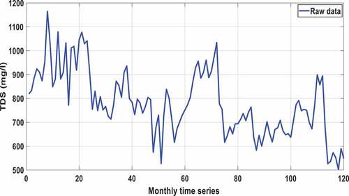
Many academics in developing countries struggle due to a lack of data. In general, Iraqi metrological stations’ data were lost due to unusual conditions (i.e. war, terrorism). Accordingly, to be with Ahmad, et al. (Ahmad et al., 2021), Capt, et al. (Capt et al., 2021) and Tiyasha, et al. (Tiyasha et al., 2021), climatic variables were collected from the National Oceanic and Atmospheric Administration(NOAA) (National Oceanic and Atmospheric Administration, 2021). The data set represent: maximum temperature (T max) (◦C), minimum temperature (T min) (◦C), mean temperature (T mean) (◦C), dew point (Dew) (°C), pressure (P) (kPa), rainfall (Rain) (mm/day), wind speed (W) (m/sec), wind range (W range) (m/sec), wind maximum (W max) (m/sec), wind minimum (W min) (m/sec), relative humidity (RH) (%) and specific humidity (SH) (%). Figure 1 shows the raw time series of monthly (TDS) data.

Figure 1. Raw monthly time series of water quality parameters (TDS).

3. Methodology

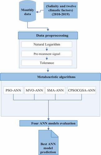
The proposed methodology can be divided into four stages: data pre-processing, artificial neural network, CPSOCGSA algorithm, and model evaluation. The architecture of the proposed methodology for forecasting monthly water quality parameters based on meteorological data is shown in Figure 2.

Figure 2. A scheme of suggested methodology to forecast monthly salinity time series.

3.1. Data pre-processing

The data pre-processing technique followed in this work comprises three approaches: normalisation, cleaning and selecting the best model input.

3.1.1. Normalisation

The natural logarithm method (Equation 1(1) $X_{normalised}=\mathrm{l}\mathrm{n}\left(X_{raw}\right)$(1) ) was employed in this work to normalise the data to be more stable and reduce collinearity between the independent factors (Zubaidi et al., 2022). It is performed by using the SPSS 24 statistics package.

(1) $X_{normalised}=\mathrm{l}\mathrm{n}\left(X_{raw}\right)$(1)

X = dependent and independent time series.

3.1.2. Cleaning

Data cleaning strategies include detecting and treating outliers. After that, removing noise to improve the data analysis results. Outliers’ data have negative effect on the model accuracy (Zubaidi, Gharghan, et al., 2018). The box and whisker approach was used to identify outliers data that lie beyond the range ±1.5 IQR (IQR = 3^rd quartile (Q3)—1^st quartile (Q1)) (Kossieris & Makropoulos, 2018). The SPSS 24 statistics package was used to apply this approach, and the singular spectrum analysis (SSA) was used for denoising time series after detecting and treating the outliers.

SSA is a relatively effective approach for decomposing the original time series into multiple principal components (PCs). Every PC explains a proportion of the variance of the original time series where the first component has the largest value, and the last component has the lowest proportion. SSA can be used for time series denoising by selecting the PCs with the largest proportions of variance and neglecting the PCs with the smallest variance proportions, which usually explain the structure-less noise in the time series. This can be conducted by using a scree-plot, which is a visualisation of the eigenvalues contained in the PCs. Mathematically, a time-series of (n) points can be decomposed, using SSA, into a number of components which is no more than half of (n). So, an analysis can start with three PCs and then be increased gradually until the best solution is obtained (Hassani, 2007; Kilundu et al., 2011).

SSA operates with both linear and nonlinear time series and decent sample sizes (Zubaidi, Dooley, et al., 2018). It detects and removes noise from data to optimise the regression coefficient and minimise the error scale (Al-Bugharbee & Trendafilova, 2016). This strategy has proven to be useful in a variety of issues, including groundwater prediction (Polomčić et al., 2017), hydrology field (Sun et al., 2018; Unnikrishnan & Jothiprakash, 2018), economics (Hassani et al., 2015), and draught (Pham et al., 2021). Additional details about SSA can be found in Golyandina and Zhigljavsky (Golyandina & Zhigljavsky, 2013).

3.1.3. Identifying explanatory variables

Selecting appropriate predictors’ scenarios is one of the most significant aspects of constructing a prediction model’s structure. Also, it improves the model’s performance (Shah et al., 2021). A tolerance method and cross-correlation will be used to determine the optimum predictor scenario without multi-collinearity between independent variables. Pallant (Pallant, 2005) recommended choosing predictors with a tolerance coefficient of 0.2 or more to ensure that there was no collinearity.

3.2. Hybridised methodology CCPSOCGSA

It combines the constriction-based particle swarm optimisation and the chaotic gravitational search algorithm to overcome the randomisation, intensification and local minima issues of standard GSA and PSO. This section will explore the component of the present hybridised methodology.

3.2.1. Constriction coefficient-based particle swarm optimisation (CCPSO)

The PSO is a popular optimisation algorithm inspired by the behaviour of fishes and birds swarms. The PSO algorithm structure has three important operators, namely, inertia weight, pbest and gbest. The inertia weight operator plays an important role in the global exploration process while the gbest and pbest help the finding of the search space region. The updating process of the location and velocity of the particles during the change of their values (particle values) can be mathematically described as in below:

(2) $v_x^d\left(t+1\right)=w\left(t\right)v_x^d\left(t\right)+c_1{r}_{x1}\left(pbes{t}_x-x_x^d\left(t\right)\right)+c_2{r}_{x2}\left(gbest-x_x^d\left(t\right)\right)$(2)

(3) $x_x^d\left(t+1\right)=x_x^d\left(t\right)+v_x^d\left(t+1\right)$(3)

The $c_1,c_2$ are learning constants while $r_{x1}and{r}_{x2}$ are numbers ranging from 0 to 1.

To overcome the consequences of the particle movements outside the solution space and to accelerate the convergence during the optimisation process, constriction coefficients were introduced to improve the exploitation stage of PSO (Clerc & Kennedy, 2002). The constriction coefficient is described as below:

(4) ${\phi }_1=2.05,{\phi }_2=2.05,\phi ={\phi }_1+{\phi }_2$(4)

(5) $K=2/\left(\phi -2+\sqrt{\left({\phi }^2-4\right)}\right)$(5)

Where K is the constriction coefficient and represents the inertia weight. Equation (2)(2) $v_x^d\left(t+1\right)=w\left(t\right)v_x^d\left(t\right)+c_1{r}_{x1}\left(pbes{t}_x-x_x^d\left(t\right)\right)+c_2{r}_{x2}\left(gbest-x_x^d\left(t\right)\right)$(2) can be rewritten as below:

(6) $v_x^d\left(t+1\right)=K{v}_x^d\left(t\right)+K{\phi }_1{r}_{x1}\left(pbes{t}_x\left(t\right)-x_x^d\left(t\right)\right)+K{\phi }_2{r}_{x2}\left(gbest-x_x^d\left(t\right)\right)$(6)

Where $K{\phi }_1=c_1$, $K{\phi }_2=c_2$

3.2.2. Chaotic gravitational search algorithm CGSA

GSA is one of the optimisation techniques that are inspired by physical phenomena. More specifically, it is inspired by Newton’s law of gravitation and motion. This technique starts by initialising the optimisation process by representing the searching agents as masses. The gravitational force $F_{ij}$ between masses (i.e. searching agents) x and y at time t can be represented as in the following Equation (7)(7) $F_{xy}=G\left(t\right)\frac{m_{px}\left(t\right)m_{ay}\left(t\right)}{R_{xy}\left(t\right)+\in }\left(x_x^d\left(t\right)+x_y^d\left(t\right)\right)$(7) :

(7) $F_{xy}=G\left(t\right)\frac{m_{px}\left(t\right)m_{ay}\left(t\right)}{R_{xy}\left(t\right)+\in }\left(x_x^d\left(t\right)+x_y^d\left(t\right)\right)$(7)

Where $m_{px}and{m}_{ay}$ represent attractive and passive masses, respectively. The R_xy(t) represents the Euclidian distance between the two masses at time t while $\in$ is a small coefficient. The constant G helps in controlling the solution space and finding the feasible region and can be represented by Equation (8)(8) $G\left(t\right)=G\left(t_o\right)e^{\left(-\alpha \frac{CI}{MI}\right)}$(8) :

(8) $G\left(t\right)=G\left(t_o\right)e^{\left(-\alpha \frac{CI}{MI}\right)}$(8)

Where $G\left(t\right)\mathrm{\&}G\left(t_o\right)$ are the final and initial values of G, $\alpha$ is a small constant, $CI$ is the current iteration, and $MI$ is the maximum number of iterations.

The change of G over time is described using a chaotic normalisation process (Rather & Bala, ,), and the final representation of the gravitational constant can be represented by the Equation (9)(9) $G^c\left(t\right)=C_i^{norm}\left(t\right)+G\left(t_o\right)e^{\left(-\alpha \frac{CI}{MI}\right)}$(9) :

(9) $G^c\left(t\right)=C_i^{norm}\left(t\right)+G\left(t_o\right)e^{\left(-\alpha \frac{CI}{MI}\right)}$(9)

The total force exerted by the masses (i.e. searching agents) can be described as in Equation (10)(10) $F_x^d\left(t\right)=\sum _{y=1,y\ne x}^m{\gamma }_y{F}_{xy}$(10) below:

(10) $F_x^d\left(t\right)=\sum _{y=1,y\ne x}^m{\gamma }_y{F}_{xy}$(10)

Where $\gamma$ is a constant range between 0 and 1.

It is important to calculate the position and velocity of the heavy search agent (i.e. mass) for the purpose of finding the global optimum. The position and velocity can be represented according to Equation (11)(11) $v_x^d\left(t+1\right)={\gamma }_y{v}_x^d\left(t\right)+a_x^d\left(t\right)$(11) and (12(12) $x_x^d\left(t+1\right)=x_x^d\left(t\right)+v_x^d\left(t+1\right)$(12) ):

(11) $v_x^d\left(t+1\right)={\gamma }_y{v}_x^d\left(t\right)+a_x^d\left(t\right)$(11)

(12) $x_x^d\left(t+1\right)=x_x^d\left(t\right)+v_x^d\left(t+1\right)$(12)

Where $a_x^d\left(t\right)$ is the acceleration of the mass.

3.2.3. Combination of CCPSO and CGSA

Combining the CPSO and CGSA means combining the diversification and convergence properties of the two techniques. The hybridisation equation formula can be described as in Equation (13)(13) $v_x^d\left(t+1\right)=\left(2/\left(\phi -2+\sqrt{{\phi }^2-4}\right)\right)v_x^d\left(t\right)+K{\phi }_1{r}_{x1}\left(a_x^d\left(t\right)-x_x^d\left(t\right)\right)+K{\phi }_2{r}_{x2}\left(gbest-x_x^d\left(t\right)\right)$(13) :

(13) $v_x^d\left(t+1\right)=\left(2/\left(\phi -2+\sqrt{{\phi }^2-4}\right)\right)v_x^d\left(t\right)+K{\phi }_1{r}_{x1}\left(a_x^d\left(t\right)-x_x^d\left(t\right)\right)+K{\phi }_2{r}_{x2}\left(gbest-x_x^d\left(t\right)\right)$(13)

And the location of the particles is given by Equation (14)(14) $x_x^d\left(t+1\right)=x_x^d\left(t\right)+v_x^d\left(t+1\right)$(14) :

(14) $x_x^d\left(t+1\right)=x_x^d\left(t\right)+v_x^d\left(t+1\right)$(14)

3.3. Artificial neural network (ANN)

ANN is an information processing system simulating human brain processes using the same connectivity and behaviour as biological neurons (Hussaini et al., 2020). In this work, a multilayer perceptron (MLP) network was employed (a feed-forward (FF), backpropagation network) along with the Levenberg-Marquardt learning method (LM) to train ANN, as in Csábrági, et al. (Csábrági et al., 2017). Thomas, et al. (Thomas et al., 2017) examined whether or not using MLFFNN with two hidden layers enhances generalisation in comparison to using a single hidden layer. The research found that two-layer networks performed better as generalises nine times out of ten. Additionally, various research have shown that ANNs with two hidden layers effectively represent the nonlinear connection between the simulated and observed, such as water quality (Deng et al., 2021), draught (Mulualem & Liou, 2020), and water demand (González Perea et al., 2019). Accordingly, the proposed ANN structure consists of four layers of neurons: an input layer that has the independent factors; two hidden layers to deal with the complex nonlinearity of time series; and an output layer that contains dependent factors (target).

To improve extrapolation outside the range of the training data, Noori,et al. (Noori et al., 2011) suggested using sigmoidal type transfer functions in the hidden layer and linear transfer functions in the output layer. Also, the tansigmoidal activation function was recommended for pattern recognition issues (Hagan et al., 2019). Moreover, when a neural network tackles a regression problem, all the neurons in the output layer must have a linear activation function (Noori et al., 2011). So, this research uses tansigmoidal and linear activation functions for both hidden and output layers, respectively. The model was implemented using the MATLAB Neural Network Toolbox. More details about ANN can see in Hagan, et al. (Hagan et al., 2019). Ann is effective in a variety of hydrological applications, including simultaneous management of water and wastewater (Rastegaripour et al., 2018), streamflow prediction (Huang et al., 2021), and drought forecasting (Ahmadi et al., 2021). To produce optimal input/output mapping and avoid over-and under-estimation, a metaheuristic algorithm was combined with ANN to choose the optimum number of neurons in the hidden layers (N1 and N2) and the best learning rate coefficient (LR).

The data were divided into three sets: training, testing, and validation, with 70%, 15%, and 15% of samples used for each group, respectively, as was done previously in Kulisz, et al. (Kulisz et al., 2021) and Zubaidi, et al. (Zubaidi, Gharghan, et al., 2018).

3.4. Performance measurement criteria

It is essential to select suitable statistical metrics for specific applications because there are no global performance metrics (Y. Seo et al., 2018). Different statistical criteria are employed to express the degree of agreement between simulated and actual data. Accordingly, five statistical performance indicators were computed and categorised into absolute error, relative error and dimensionless (Zubaidi et al., 2022). The absolute error comprises the root mean square error (RMSE, Equation 15)(15) $\mathrm{R}\mathrm{M}\mathrm{S}\mathrm{E}=\sqrt{\frac{{\sum }_{\mathrm{i}=1}^{\mathrm{N}}{\left({\mathrm{O}}_{\mathrm{i}}-{\mathrm{F}}_{\mathrm{i}}\right)}^2}{\mathrm{N}}}$(15) and mean absolute errors (MAE, Equation 16)(16) $\mathrm{M}\mathrm{A}\mathrm{E}=\frac{{\sum }_{\mathrm{i}=1}^{\mathrm{N}}\left|{\mathrm{O}}_{\mathrm{i}}-{\mathrm{F}}_{\mathrm{i}}\right|}{\mathrm{N}}$(16) . The relative error is represented by the mean absolute relative error (MARE, Equation 17(17) $MARE=\frac{1}{N}\sum _{i=1}^N\frac{\left|O_i-F_i\right|}{O_i}$(17) ), and the dimensionless criteria contain the determination coefficient (R², Equation 18)(18) ${R^2}^{=}{\left[\frac{{\sum }_{i=1}^N\left(O_i-{\bar{O}}_i\right)\left(F_i-{\bar{F}}_i\right)}{\sqrt{{\sum }^{{\left(O_i-{\bar{O}}_i\right)}^2}{\sum }^{{\left(F_i-{\bar{F}}_i\right)}^2}}}\right]}^2$(18) and scatter index (SI, Equation 19)(19) $SI=\frac{RMSE}{\bar{O}}\times 100$(19) .

(15) $\mathrm{R}\mathrm{M}\mathrm{S}\mathrm{E}=\sqrt{\frac{{\sum }_{\mathrm{i}=1}^{\mathrm{N}}{\left({\mathrm{O}}_{\mathrm{i}}-{\mathrm{F}}_{\mathrm{i}}\right)}^2}{\mathrm{N}}}$(15)

(16) $\mathrm{M}\mathrm{A}\mathrm{E}=\frac{{\sum }_{\mathrm{i}=1}^{\mathrm{N}}\left|{\mathrm{O}}_{\mathrm{i}}-{\mathrm{F}}_{\mathrm{i}}\right|}{\mathrm{N}}$(16)

(17) $MARE=\frac{1}{N}\sum _{i=1}^N\frac{\left|O_i-F_i\right|}{O_i}$(17)

(18) ${R^2}^{=}{\left[\frac{{\sum }_{i=1}^N\left(O_i-{\bar{O}}_i\right)\left(F_i-{\bar{F}}_i\right)}{\sqrt{{\sum }^{{\left(O_i-{\bar{O}}_i\right)}^2}{\sum }^{{\left(F_i-{\bar{F}}_i\right)}^2}}}\right]}^2$(18)

(19) $SI=\frac{RMSE}{\bar{O}}\times 100$(19)

Where $F_i$ represents simulated WQ variables, $O_i$: observed WQ variables, ${\bar{O}}_i$: mean of observed WQ variables, ${\bar{F}}_i$: mean of simulated WQ variables, $N$: length of data. The model’s performance is good when the value of R ² is greater than (0.85) (Dawson et al., 2007). The best model has values that are close to zero for the MBE, MAE, and RMSE metrics (Ahmed et al., 2019; Eze et al., 2021). Besides, the model is excellent when SI < 10%, good if it is between (10–20) %, fair if it is between (20–30) %, and poor if SI ≥ 30% (Csábrági et al., 2017).

Also, Augmented Dickey–Fuller (ADF) and Kwiatkowski–Phillips–Schmidt–Shin (KPSS) tests are applied to examine the stationary residual data. Furthermore, graphical tests to compare observed and simulated time series.

4. Results and discussion

4.1. Preparation of input and target variables

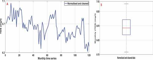
All the time series were normalised to reduce the impact of outliers and make the distribution of time series normal or close to normal, according to Tabachnick and Fidell (Tabachnick & Fidell, 2013). Then, the remind outliers (if found) were adjusted. For example, the time series and box plot for normalised and cleaned TDS time series is shown in Figure 3.

Figure 3. Water quality parameter (TDS) after normalising and cleaning, (A) Monthly time series, (B) Box plot.

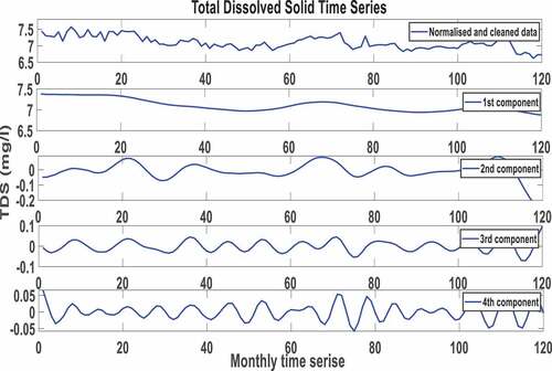
Then, the SSA technique was employed to denoise all dependent and independent time series. Figure 4 demonstrates the normalised and cleaned time series and the first four components for the TDS parameter. The 1^st component represents the time series after denoising that has the largest value of the normalised and clean time series.

Figure 4. Normalised and cleaned water time series and the first four components obtained by SSA.

In the last phase of data pre-processing, a tolerance method was applied to find the best scenario of predictor factors, which could accurately forecast the water quality parameter and omit redundant factors to avoid multi-collinearity. For the TDS model, in the initial stage, the tolerance coefficient values were lower than the acceptable limit (i.e. it should be equal to or more than 0.2). Accordingly, extensive scenarios were performed until the tolerance values of the selected predictors reached equal or more than 0.2, as shown in Table 1. The latter indicates that TDS_t-1, P, Tmax, RH, and Wmax were chosen as the best independent factors scenario based on the tolerance value. In the same procedure, for the EC model, EC_t-1, P, RH, and Tmax were selected as the best independent factors scenario based on the tolerance value. As presented in Table 1, for both models, the tolerance coefficient value for each predictor was more than 0.2, which means the multi-collinearity assumption was not violated. In addition, Table 1 shows that several factors contribute to establishing how climate affects water salinity. These findings corroborate the negative effects of climate change on river water quality that have been documented in the literature.

Table 1. Collinearity statistics for the specified predictors

Parameter	Independent variables	Tolerance value
TDS	TDSt-1	0.227
	P	0.317
	T max	0.393
	RH	0.460
	W max	0.490
EC	ECt-1	0.245
	P	0.324
	RH	0.461
	T max	0.673

After pre-processing raw data, the correlation coefficients between dependent and independent factors are improved. The correlation coefficients between TDS and EC and their first lag time series significantly increased from 0.788 to 0.997 and 0.805 to 0.997, respectively. That results from improving the quality of raw time series due to treating the outliers data and noise removal. Accordingly, the prediction accuracy will increase and reduce the scale of error.

Before configuring the prediction model, data were organised into three sets: training (70%, 83 data points), testing (15%, 18 data points) and validation (15%, 18 data points).

4.2. Configuring the model

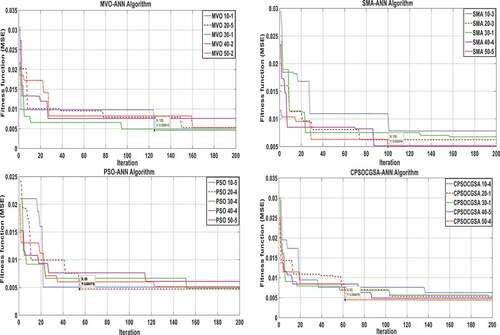
The systematic configuration of the ANN approach rather than a trial-and-error procedure is vital for building a precise water quality forecast model. Accordingly, four hybrid metaheuristic algorithms (CPSOCGSA-ANN, PSO-ANN, MVO-ANN, and SMA-ANN) were applied to determine the optimum hyperparameters (Lr, N1, and N2) of the ANN approach. In this study, five swarm sizes (10, 20, 30, 40, and 50) were attempted by combining various algorithms with ANN. Each swarm for each algorithm was performed five times to obtain the optimum solution (e.g., see Figure S1 for modelling TDS, CPSOCGSA-ANN algorithm).

After that, the optimum swarm for each algorithm was nominated to compare it with other swarms for the same algorithm, as depicted in Figures 5 and 6 for TDS and EC models, respectively. Figure 5 shows that the best swarms for the TDS model are 10–1 for MVO-ANN, 40–1 for PSO-ANN, and 50–4 for SMA-ANN and CPSOCGSA-ANN algorithms. Besides, from Figure 6, the best swarms for the EC model are 10–1 for MVO-ANN, 50–5 for SMA-ANN, 20–4 for PSO-ANN, and 50–4 for CPSOCGSA-ANN algorithms.

Figure 5. Performance of PSO-ANN, SMA-ANN, CPSOCGSA-ANN and MVO-ANN algorithms for TDS modelling.

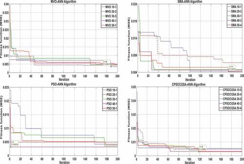
Figure 6. Performance of PSO-ANN, SMA-ANN, CPSOCGSA-ANN and MVO-ANN algorithms for EC modelling.

The optimal ANN hyperparameters derived from the CPSOCGSA-ANN, SMA-ANN, PSO-ANN, and MVO-ANN algorithms, are presented in Table 2.

Table 2. ANN hyperparameters based on four metaheuristic algorithms

Parameter	Hyperparameter	CPSOCGSA-ANN	SMA-ANN	MVO-ANN	PSO-ANN
TDS	LR	0.2673	0.6834	0.8571	0.1341
	N1	6	15	19	5
	N2	5	2	1	4
EC	LR	0.2397	0.8140	0.3356	0.4028
	N1	3	15	10	11
	N2	3	9	1	5

4.3. Forecasting results of various algorithms

To be with Tao, et al. (Tao et al., 2021) and Ghorbani, et al. (Ghorbani et al., 2018) procedure, four ANN techniques were configured depending on the hyperparameters in Table 2. Each ANN model was run multiple times to locate the best network that provides a precise solution. Four statistical criteria were utilised to examine the models’ performance (see Section 3.4 for more details). Table 3 displays the statistical criteria for each hybrid model for the TDS and EC prediction model. For the TDS model, the CPSOCGSA-ANN, PSO-ANN, and MVO-ANN techniques yielded R² of more than 0.85, which means good results, according to Dawson, et al. (Dawson et al., 2007). However, CPSOCGSA-ANN tends to perform better than the other three techniques, with an R² of 0.99. Further, CPSOCGSA-ANN is more accurate in MAE, RMSE, and MARE tests than in the other techniques, e.g., the MAE values of CPSOCGSA-ANN, PSO-ANN, MVO-ANN, and SMA-ANN are 0.0174, 0.0312, 0.0536, 0.0201, respectively. Regarding the EC model, the CPSOCGSA-ANN yielded R² = 0.97 of more than 0.85, which means good results compared with the other techniques that yielded less than 0.85. Also, it offers a lower scale of error based on MAE, RMSE, and MARE criteria; for example, the MAE values of CPSOCGSA-ANN, PSO-ANN, MVO-ANN, and SMA-ANN are 0.0137, 0.0911, 0.0586, 0.0226, respectively. What stands out in this table is highlighting the superiority of the CPSOCGSA-ANN technique (in the validation stage) concerning other techniques for forecasting TDS and EC parameters.

Table 3. Performance assessment for validation data stage

Parameter	Models	R^2	MAE (mg/l)	RMSE (mg/l)	MARE
TDS	CPSOCGSA-ANN	0.99	0.0174	0.0205	0.0027
	PSO-ANN	0.88	0.0312	0.0483	0.0048
	MVO-ANN	0.89	0.0536	0.0658	0.0082
	SMA-ANN	0.82	0.0201	0.0221	0.0031
Parameter	Models	R^2	MAE (µ mhos/cm)	RMSE (µ mhos/cm)	MARE
EC	CPSOCGSA-ANN	0.97	0.0137	0.0210	0.0020
	PSO-ANN	0.66	0.0911	0.0971	0.0138
	MVO-ANN	0.55	0.0586	0.0736	0.0080
	SMA-ANN	0.84	0.0226	0.0279	0.0032

Also, to evaluate and analyse the performance of different prediction approaches in the validation stage, the Taylor diagram was chosen. This graph depicts the agreement between observed and simulated patterns, taking into account standard deviation (SD), root mean square difference (RMSD), and the correlation coefficient (R). Figure 8 demonstrates the Taylor diagram for the TDS and EC parameters based on CPSOCGSA-ANN (A), PSO-ANN (B), MVO-ANN (C), and SMA-ANN (D) techniques. The most obvious finding to emerge from the figure is that the CPSOCGSA-ANN (A) technique (for TDS and EC parameters) produced high R and low SD and RMSD relative to a reference point, which refers to the observed pattern. The results, as shown in Figure 7, support the results of Table 3 and indicate the effectiveness of the CPSOCGSA-ANN technique in simulating the water quality parameters.

Figure 7. Taylor diagram of CPSOCGSA-ANN (A), PSO-ANN (B), MVO-AN (C), and SMA-ANN (D) predicted models for TDS and EC parameters.

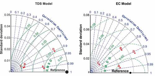
Figure 8. Box plot of predictions employed for model evaluation in the validation phase.

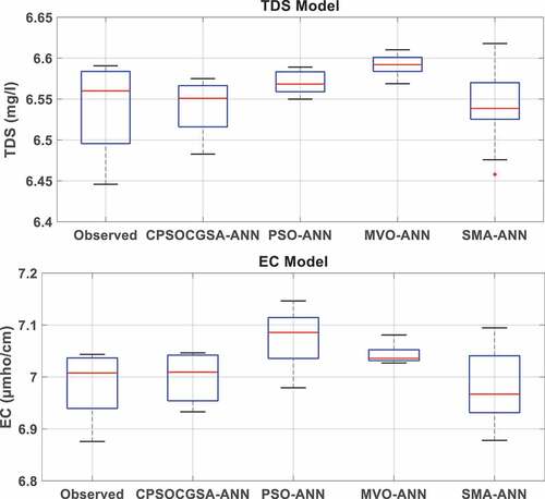
For more validation, the box plots were prepared to display the capability of the four hybrid techniques to replicate TDS and EC in the validation stage. Obtained outcomes are demonstrated in Figure 8. A hybrid technique can be considered good if it replicates the observed box reliably. The outcomes revealed the ability of the CPSOCGSA-ANN technique to replicate the observed box for TDS and EC parameters well. It was also found to replicate well the median and range of observed TDS and EC parameters in compassion with other techniques.

Overall, the CPSOCGSA-ANN technique performs well than the other hybrid techniques. A likely explanation is that this can be attributed to the combination of PSO’s exploitation skills with GSA’s exploration ones for optimal performance. Accordingly, residual analysis was used to support the CPSOCGSA-ANN technique further. The residual data are stationary according to ADF and KPSS tests. Additionally, the CPSOCGSA-ANN has an excellent performance with SI = 0.003 for TDS and EC prediction model according to the limitations in section 3.5. The most obvious findings to emerge from this study are that:

1. These findings highlight the potential usefulness of the SSA and tolerance techniques. The former technique improves raw data quality by increasing the correlation between dependent and independent variables due to removing the structure-less noise. The latter technique selects the best predictors scenario without violating the multi-collinearity assumption.

2. CPSOCGSA emerged as a reliable algorithm that is used to integrate the ANN model for forecast salinity compared with PSO, MVO, and SMA algorithms. This can be attributed to the combination of PSO’s exploitation skills with GSA’s exploration ones for optimal performance.

3. Different statistical criteria analyses (i.e. absolute error, relative error, dimensionless, residual analysis, and graphical tests) revealed that the suggested methodology accurately forecasted river water salinity.

4. The current findings clearly support the relevance of medium-term climatic and lag factors’ impact on salinity.

5. The findings of this research provide insights for applying more hybrid prediction techniques in different regions.

5. Conclusions

The goal and main contribution of the present study were to evaluate the application of a new methodology consisting of pre-processing data methods and an ANN model integrated by four different metaheuristic algorithms (SMA-ANN, CPSOCGSA-ANN, PSO-ANN and MVO-ANN) to forecast monthly water salinity (TDS and EC). TDS and EC data for the Euphrates River at al-Musayyab District and climatic data over ten years (2010–2019) were used to build and assess the proposed methodology. Based on the findings, it can be concluded that:

1. Data pre-processing techniques, SSA, and tolerance are essential for improving raw data quality and selecting the optimum model input scenario. Accordingly, extra investigations into data pre-processing techniques, such as principal component analysis, are strongly recommended.

2. CPSOCGSA-ANN is an effective technique capable of accurately forecasting water salinity and outperforming other hybrid algorithms based on several statistical tests. It yielded a higher R² and lower error (see Table 4).

3. Since there is a lot of potential for improvement in pre-treatment signal, data reduction, and identifying the hyperparameters of machine learning models, it is advised that more research be conducted in combination prediction models (HPOH).

4. The research can provide a basis for trainers, engineers, and policymakers to design and manage decision-making about rivers and basins in Iraq under climate change variability.

5. The study reveals that there is an urgent need for more research using different AI techniques coupled with the CPSOCGSA algorithm to further elaborate their performance with improved parameters in modelling other water quality parameters.

6. Another possible area of future research would be to investigate further predictors (e.g., river discharge, water level, and additional climatic factors).

Disclosure statement

No potential conflict of interest was reported by the author(s).

Additional information

Funding

This work was supported by the Lulea University of Technology [184940].

Notes on contributors

Nadhir Al-Ansari

Nadhir Al-Ansari Professor at the department of Civil, Environmental and Natural Resources Engineering at Lulea Technical University Sweden. Research interests are mainly in Water Resources and Environment. Served several academic administrative post (Dean, Head of Department). Publications include more than 790 articles in international/national journals, chapters in books and 22 books. He supervised more than 70 postgraduate students. He executed more than 60 major research projects in Iraq, Jordan, Sweden and UK. Awarded several scientific and educational awards, among them is the British Council on its 70th Anniversary awarded him top 5 scientists in Cultural Relations. One patent on Physical methods for the separation of iron oxides. Supervised more than 70 postgraduate students at different universities. Member of several scientific societies e.g. International Association of Hydrological Sciences, Chartered Institution of Water and Environment Management, Network of Iraqi Scientists Abroad, etc. Member of the editorial board of 32 international journals.

References

- Aghel, B., Rezaei, A., & Mohadesi, M. (2018). Modeling and prediction of water quality parameters using a hybrid particle swarm optimization–neural fuzzy approach. International Journal of Environmental Science and Technology, 16(8), 4823–20. https://doi.org/10.1007/s13762-018-1896-3
- Ahmadi, F., Mehdizadeh, S., & Mohammadi, B. (2021). Development of bio-inspired- and wavelet-based hybrid models for reconnaissance drought index modeling. Water Resources Management, 35(12), 4127–4147. https://doi.org/10.1007/s11269-021-02934-z
- Ahmad, H. Q., Kamaruddin, S. A., Harun, S. B., Al-Ansari, N., Shahid, S., & Jasim, R. M. (2021). Assessment of spatiotemporal variability of meteorological droughts in northern Iraq using satellite rainfall data. KSCE Journal of Civil Engineering, 25(11), 4481–4493. https://doi.org/10.1007/s12205-021-2046-x
- Ahmed, A. A. M., & Shah, S. M. A. (2017). Application of adaptive neuro-fuzzy inference system (ANFIS) to estimate the biochemical oxygen demand (BOD) of Surma River. Journal of King Saud University - Engineering Sciences, 29(3), 237–243. https://doi.org/10.1016/j.jksues.2015.02.001
- Ahmed, K., Shahid, S., Wang, X., Nawaz, N., & Najeebullah, K. (2019). Evaluation of gridded precipitation datasets over arid regions of Pakistan. Water, 11(210), 210. https://doi.org/10.3390/w11020210
- Al-Ansari, N., AlJawad, S., Adamo, N., Sissakian, V. K., Laue, J., & Knutsson, S. (2018). Water quality within the Tigris and Euphrates catchments. Journal of Earth Sciences and Geotechnical Engineering, 8, 95–121.
- Al-Bugharbee, H., & Trendafilova, I. (2016). A fault diagnosis methodology for rolling element bearings based on advanced signal pretreatment and autoregressive modelling. Journal of Sound and Vibration, 369, 246–265. https://doi.org/10.1016/j.jsv.2015.12.052
- Ali Khan, M., Izhar Shah, M., Faisal Javed, M., Ijaz Khan, M., Rasheed, S., El-Shorbagy, M. A., Roshdy El-Zahar, E., & Malik, M. Y. (2022). Application of random forest for modelling of surface water salinity. Ain Shams Engineering Journal, 13(4), 101635. https://doi.org/10.1016/j.asej.2021.11.004
- Al-Mukhtar, M., & Al-Yaseen, F. (2019). Modeling water quality parameters using data-driven models, a case study Abu-Ziriq Marsh in South of Iraq. Hydrology, 6(24), 24. https://doi.org/10.3390/hydrology6010024
- Al-Sulttani, A. O., Ahsan, A., Hanoon, A. N., Rahman, A., Daud, N. N. N., & Idrus, S. (2017). Hourly yield prediction of a double-slope solar still hybrid with rubber scrapers in low-latitude areas based on the particle swarm optimization technique. Applied Energy, 203, 280–303. https://doi.org/10.1016/j.apenergy.2017.06.011
- Al-Sulttani, A. O., Al-Mukhtar, M., Roomi, A. B., Farooque, A. A., Khedher, K. M., & Yaseen, Z. M. (2021). Proposition of new ensemble data-intelligence models for surface water quality prediction. IEEE Access, 9, 108527–108541. https://doi.org/10.1109/access.2021.3100490
- Apaydin, H., Taghi Sattari, M., Falsafian, K., & Prasad, R. (2021). Artificial intelligence modelling integrated with singular spectral analysis and seasonal-trend decomposition using Loess approaches for streamflow predictions. Journal of Hydrology, 600, 126506. https://doi.org/10.1016/j.jhydrol.2021.126506
- Asadollahfardi, G., Taklify, A., & Ghanbari, A. (2012). Application of artificial neural network to predict TDS in Talkheh Rud River. Journal of Irrigation and Drainage Engineering, 138(4), 363–370. https://doi.org/10.1061/(asce)ir.1943-4774.0000402
- Azad, A., Karami, H., Farzin, S., Mousavi, S.-F., & Kisi, O. (2019). Modeling river water quality parameters using modified adaptive neuro fuzzy inference system. Water Science and Engineering, 12(1), 45–54. https://doi.org/10.1016/j.wse.2018.11.001
- Baek, -S.-S., Pyo, J., & Chun, J. A. (2020). Prediction of water level and water quality using a CNN-LSTM combined deep learning approach. Water, 12(12), 3399. https://doi.org/10.3390/w12123399
- Barzegar, R., Aalami, M. T., & Adamowski, J. (2020). Short-term water quality variable prediction using a hybrid CNN–LSTM deep learning model. Stochastic Environmental Research and Risk Assessment, 34(2), 415–433. https://doi.org/10.1007/s00477-020-01776-2
- Barzegar, R., Adamowski, J., & Moghaddam, A. A. (2016). Application of wavelet-artificial intelligence hybrid models for water quality prediction: A case study in Aji-Chay River, Iran. Stochastic Environmental Research and Risk Assessment, 30(7), 1797–1819. https://doi.org/10.1007/s00477-016-1213-y
- Capt, T., Mirchi, A., Kumar, S., & Walker, W. S. (2021). Urban water demand: Statistical optimization approach to modeling daily demand. Journal of Water Resources Planning and Management, 147(2), 04020105. https://doi.org/10.1061/(asce)wr.1943-5452.0001315
- Chabuk, A. J., Al-Ansari, N., Hussain, H. M., Knutsson, S., & Pusch, R. (2017). GIS-based assessment of combined AHP and SAW methods for selecting suitable sites for landfill in Al-Musayiab Qadhaa, Babylon, Iraq. Environmental Earth Sciences, 76(5), 209. https://doi.org/10.1007/s12665-017-6524-x
- Chen, S., Fang, G., Huang, X., & Zhang, Y. (2018). Water quality prediction model of a water diversion project based on the improved artificial bee colony–backpropagation neural network. Water, 10(6), 806. https://doi.org/10.3390/w10060806
- Chen, Y., Song, L., Liu, Y., Yang, L., & Li, D. (2020). A review of the artificial neural network models for water quality prediction. Applied Sciences, 10(5776). https://doi.org/10.3390/app10175776
- Chyad, M. H., Gharghan, S. K., Hamood, H. Q., Altayyar, A. S. H., Zubaidi, S. L., & Ridha, H. M. (2022). Hybridization of soft-computing algorithms with neural network for prediction obstructive sleep apnea using biomedical sensor measurements. Neural Computing and Applications, 34(11), 8933–8957. https://doi.org/10.1007/s00521-022-06919-w
- Clerc, M., & Kennedy, J. (2002). The particle swarm-explosion, stability, and convergence in a multidimensional complex space. 6, 58–73. https://doi.org/10.1109/4235.985692
- Csábrági, A., Molnár, S., Tanos, P., & Kovács, J. (2017). Application of artificial neural networks to the forecasting of dissolved oxygen content in the Hungarian section of the river Danube. Ecological Engineering, 100, 63–72. https://doi.org/10.1016/j.ecoleng.2016.12.027
- Dawson, C. W., Abrahart, R. J., & See, L. M. (2007). HydroTest: A web-based toolbox of evaluation metrics for the standardised assessment of hydrological forecasts. Environmental Modelling & Software, 22(7), 1034–1052. https://doi.org/10.1016/j.envsoft.2006.06.008
- Deng, B., Lai, S. H., Jiang, C., Kumar, P., El-Shafie, A., & Chin, R. J. (2021). Advanced water level prediction for a large-scale river–lake system using hybrid soft computing approach: A case study in Dongting Lake, China. Earth Science Informatics, 14(4), 1987–2001. https://doi.org/10.1007/s12145-021-00665-8
- Dey, S., Barton, A., Kandra, H., Bagirov, A., & Wilson, K. (2021). Analysis of water quantity and quality trade-offs to inform selective harvesting of inflows in complex water resource systems. Water Resources Management, 35(12), 4149–4165. https://doi.org/10.1007/s11269-021-02936-x
- Eiben, A. E., & Schippers, C. A. (1998). On evolutionary exploration and exploitation. Fundamenta Informaticae, 35(1–4), 35–50. https://doi.org/10.3233/FI-1998-35123403
- Ethaib, S., Zubaidi, S. L., Al-Ansari, N., & Fegade, S. L. (2022). Evaluation water scarcity based on GIS estimation and climate-change effects: A case study of Thi-Qar Governorate, Iraq. Cogent Engineering, 9(1), 2075301. https://doi.org/10.1080/23311916.2022.2075301
- Ewaid, S., Abed, S., Al-Ansari, N., & Salih, R. (2020). Development and evaluation of a water quality index for the Iraqi rivers. Hydrology, 7(3), 67. https://doi.org/10.3390/hydrology7030067
- Eze, E., Halse, S., & Ajmal, T. (2021). Developing a novel water quality prediction model for a South African aquaculture farm. Water, 13(13), 1782. https://doi.org/10.3390/w13131782
- Faloye, O. T., Ajayi, A. E., Ajiboye, Y., Alatise, M. O., Ewulo, B. S., Adeosun, S. S., Babalola, T., & Horn, R. (2022). Unsaturated hydraulic conductivity prediction using artificial intelligence and multiple linear regression models in biochar amended sandy clay loam soil. Journal of Soil Science and Plant Nutrition, 22(2), 1589–1603. https://doi.org/10.1007/s42729-021-00756-x
- Ghorbani, M. A., Deo, R. C., Karimi, V., Kashani, M. H., & Ghorbani, S. (2018). Design and implementation of a hybrid MLP-GSA model with multi-layer perceptron-gravitational search algorithm for monthly lake water level forecasting. Stochastic Environmental Research and Risk Assessment, 33(1), 125–147. https://doi.org/10.1007/s00477-018-1630-1
- Giri, S. (2021). Water quality prospective in Twenty First Century: Status of water quality in major river basins, contemporary strategies and impediments: A review. environmental Pollution, 271, 116332. https://doi.org/10.1016/j.envpol.2020.116332
- Golyandina, N., & Zhigljavsky, A. (2013). Singular spectrum analysis for time series. Springer.
- González Perea, R., Camacho Poyato, E., Montesinos, P., & Rodríguez Díaz, J. A. (2019). Optimisation of water demand forecasting by artificial intelligence with short data sets. Biosystems Engineering, 177, 59–66. https://doi.org/10.1016/j.biosystemseng.2018.03.011
- Hagan, M., Demuth, H., Hudson Beale, M., & Jesús, O. (2019). Neural Network Design 2nd ed. eBook. 1012
- Hajirahimi, Z., & Khashei, M. (2022). Hybridization of hybrid structures for time series forecasting: A review. Artificial Intelligence Review, 2022. https://doi.org/10.1007/s10462-022-10199-0
- Han, K., & Wang, Y. (2021). A review of artificial neural network techniques for environmental issues prediction. Journal of Thermal Analysis and Calorimetry, 145(4), 2191–2207. https://doi.org/10.1007/s10973-021-10748-9
- Hassani, H. (2007). Singular spectrum analysis: Methodology and comparison. Journal of Data Science, 5(2), 239–257. https://doi.org/10.6339/JDS.2007.05(2).396
- Hassani, H., Webster, A., Silva, E. S., & Heravi, S. (2015). Forecasting U.S tourist arrivals using optimal singular spectrum analysis. Tourism Management, 46, 322–335. https://doi.org/10.1016/j.tourman.2014.07.004
- Hien Than, N., Dinh Ly, C., & Van Tat, P. (2021). The performance of classification and forecasting Dong Nai River water quality for sustainable water resources management using neural network techniques. Journal of Hydrology, 596, 126099. https://doi.org/10.1016/j.jhydrol.2021.126099
- Houssein, E. H., Mahdy, M. A., Blondin, M. J., Shebl, D., & Mohamed, W. M. (2021). Hybrid slime mould algorithm with adaptive guided differential evolution algorithm for combinatorial and global optimization problems. Expert Systems with Applications, 174, 114689. https://doi.org/10.1016/j.eswa.2021.114689
- Huang, X., Li, Y., Tian, Z., Ye, Q., Ke, Q., Fan, D., Mao, G., Chen, A., & Liu, J. (2021). Evaluation of short-term streamflow prediction methods in Urban river basins. Physics and Chemistry of the Earth, Parts A/B/C, 123, 103027. https://doi.org/10.1016/j.pce.2021.103027
- Hunter, J. M., Maier, H. R., Gibbs, M. S., Foale, E. R., Grosvenor, N. A., Harders, N. P., & Kikuchi-Miller, T. C. (2018). Framework for developing hybrid process-driven, artificial neural network and regression models for salinity prediction in river systems. Hydrology and Earth System Sciences, 22(5), 2987–3006. https://doi.org/10.5194/hess-22-2987-2018
- Hussaini, A., Mahmud, M. R., Wee, K. T. K., & Abubakar, A. G. (2020). A review of water level fluctuation models and modelling initiatives. Journal of Computational and Theoretical Nanoscience, 17(2), 645–653. https://doi.org/10.1166/jctn.2020.8781
- Jackson-Blake, L., Clayer, F., Haande, S., Sample, J., & Moe, J. (2022). Seasonal forecasting of lake water quality and algal bloom risk using a continuous Gaussian Bayesian network. Hydrology and Earth System Sciences, 26(12), 3103–3124. https://doi.org/10.5194/hess-2021-621
- Jamei, M., Ahmadianfar, I., Karbasi, M., Jawad, A. H., Farooque, A. A., & Yaseen, Z. M. (2021). The assessment of emerging data-intelligence technologies for modeling Mg(+2) and SO4(−2) surface water quality. journal of Environmental Management, 300, 113774. https://doi.org/10.1016/j.jenvman.2021.113774
- Jones, E., & van Vliet, M. T. H. (2018). Drought impacts on river salinity in the southern US: Implications for water scarcity. science of the Total environment, 644, 844–853. https://doi.org/10.1016/j.scitotenv.2018.06.373
- Kadkhodazadeh, M., & Farzin, S. (2021). A novel LSSVM model integrated with GBO algorithm to assessment of water quality parameters. Water Resources Management, 35(12), 3939–3968. https://doi.org/10.1007/s11269-021-02913-4
- Kamel, A. H., Sulaiman, M. A., & Mustaffa, A. S. (2013). Study of the effects of water level depression in Euphrates river on the water quality. Journal of Civil Engineering and Architecture, 7, 238–247.
- Khudhair, Z. S., Zubaidi, S. L., Ortega-Martorell, S., Al-Ansari, N., Ethaib, S., & Hashim, K. (2022). A review of hybrid soft computing and data pre-processing techniques to forecast freshwater quality’s parameters: current trends and future directions. Environments, 9(85), 85. https://doi.org/10.3390/environ-ments9070085
- Kilinc, H. C., & Yurtsever, A. (2022). Short-term streamflow forecasting using hybrid deep learning model based on grey wolf algorithm for hydrological time series. Sustainability, 14(6), 3352. https://doi.org/10.3390/su14063352
- Kilundu, B., Chiementin, X., & Dehombreux, P. (2011). Singular spectrum analysis for bearing defect detection. Journal of Vibration and Acoustics, 133(5), 1–7. https://doi.org/10.1115/1.4003938
- Kossieris, P., & Makropoulos, C. (2018). Exploring the statistical and distributional properties of residential water demand at fine time scales. Water, 10(10), 1481. https://doi.org/10.3390/w10101481
- Kulisz, M., Kujawska, J., Przysucha, B., & Cel, W. (2021). Forecasting water quality index in groundwater using artificial neural network. Energies, 14(18), 5875. https://doi.org/10.3390/en14185875
- Kumar, C., Raj, T. D., Premkumar, M., & Raj, T. D. (2020). A new stochastic slime mould optimization algorithm for the estimation of solar photovoltaic cell parameters. Optik, 223, 165277. https://doi.org/10.1016/j.ijleo.2020.165277
- Li, S., Chen, H., Wang, M., Heidari, A. A., & Mirjalili, S. (2020). Slime mould algorithm: A new method for stochastic optimization. Future Generation Computer Systems, 111, 300–323. https://doi.org/10.1016/j.future.2020.03.055
- Li, W., Fang, H., Qin, G., Tan, X., Huang, Z., Zeng, F., Du, H., & Li, S. (2020). Concentration estimation of dissolved oxygen in Pearl River Basin using input variable selection and machine learning techniques. Science of the Total Environment, 731, 139099. https://doi.org/10.1016/j.scitotenv.2020.139099
- Melesse, A. M., Khosravi, K., Tiefenbacher, J. P., Heddam, S., Kim, S., Mosavi, A., & Pham, B. T. (2020). River water salinity prediction using hybrid machine learning models. Water, 12(10), 2951. https://doi.org/10.3390/w12102951
- Mirjalili, S., Mirjalili, S. M., & Hatamlou, A. (2015). Multi-verse optimizer: A nature-inspired algorithm for global optimization. Neural Computing and Applications, 27(2), 495–513. https://doi.org/10.1007/s00521-015-1870-7
- Mulualem, G. M., & Liou, Y.-A. (2020). Application of artificial neural networks in forecasting a standardized precipitation evapotranspiration index for the upper Blue Nile Basin. Water, 12(3), 643. https://doi.org/10.3390/w12030643
- Nabipour, N., Dehghani, M., Mosavi, A., & Shamshirband, S. (2020). Short-term hydrological drought forecasting based on different nature-inspired optimization algorithms hybridized with artificial neural networks. IEEE Access, 8, 15210–15222. https://doi.org/10.1109/access.2020.2964584
- Najah Ahmed, A., Binti Othman, F., Abdulmohsin Afan, H., Khaleel Ibrahim, R., Ming Fai, C., Shabbir Hossain, M., Ehteram, M., & Elshafie, A. (2019). Machine learning methods for better water quality prediction. Journal of Hydrology, 578, 124084. https://doi.org/10.1016/j.jhydrol.2019.124084
- Najah, A., El-Shafie, A., Karim, O. A., & El-Shafie, A. H. (2013). Application of artificial neural networks for water quality prediction. Neural computing and Applications, 22(S1), S187–S201. https://doi.org/10.1007/s00521-012-0940-3
- National Oceanic and Atmospheric Administration. (2021). Data tools: Find a station. https://www.ncdc.noaa.gov/cdo-web/datatools/findstation (accessed 1 December 2021).
- Noori, R., Karbassi, A. R., Mehdizadeh, H., Vesali-Naseh, M., & Sabahi, M. S. (2011). A framework development for predicting the longitudinal dispersion coefficient in natural streams using an artificial neural network. Environmental Progress & Sustainable Energy, 30(3), 439–449. https://doi.org/10.1002/ep.10478
- Osman, Y., Abdellatif, M., Al-Ansari, N., Knutsson, S., & Jawad, S. (2017). Climate change and future precipitation in an arid environment of the Middle East: Case study of Iraq. Journal of Environmental Hydrology, 25, 1–18.
- Pallant, J. (2005). SPSS Survival Manual: A step by step guide to data analysis using SPSS for Windows (Version 12). Open University Press/McGraw-Hill: Aotearoa.
- Panyadee, P., Champrasert, P., & Aryupong, C. (2017). Water level prediction using artificial neural network with particle swarm optimization model. In Proceedings of 2017 Fifth International Conference on Information and Communication Technology (ICoICT), Melaka, Malaysia. IEEE.
- Peng, T., Zhou, J., Zhang, C., & Fu, W. (2017). Streamflow forecasting using empirical wavelet transform and artificial neural networks. Water, 9(6), 406. https://doi.org/10.3390/w9060406
- Pham, Q. B., Yang, T.-C., Kuo, C.-M., Tseng, H.-W., & Yu, P.-S. (2021). Coupling singular spectrum analysis with least square support vector machine to improve accuracy of SPI drought forecasting. Water Resources Management, 35(3), 847–868. https://doi.org/10.1007/s11269-020-02746-7
- Polomčić, D., Gligorić, Z., Bajić, D., & Cvijović, Č. (2017). A hybrid model for forecasting groundwater levels based on Fuzzy C-mean clustering and singular spectrum analysis. Water, 9(7), 541. https://doi.org/10.3390/w9070541
- Raheli, B., Aalami, M. T., El-Shafie, A., Ghorbani, M. A., & Deo, R. C. (2017). Uncertainty assessment of the multilayer perceptron (MLP) neural network model with implementation of the novel hybrid MLP-FFA method for prediction of biochemical oxygen demand and dissolved oxygen: A case study of Langat River. Environmental Earth Sciences, 76(14), 503. https://doi.org/10.1007/s12665-017-6842-z
- Rahi, K. A., & Halihan, T. (2009). Changes in the salinity of the Euphrates River system in Iraq. Regional Environmental Change, 10(1), 27–35. https://doi.org/10.1007/s10113-009-0083-y
- Rajaee, T., Khani, S., & Ravansalar, M. (2020). Artificial intelligence-based single and hybrid models for prediction of water quality in rivers: A review. Chemometrics and Intelligent Laboratory Systems, 200, 103978. https://doi.org/10.1016/j.chemolab.2020.103978
- Rastegaripour, F., Saboni, M. S., Shojaei, S., & Tavassoli, A. (2018). Simultaneous management of water and wastewater using ant and artificial neural network (ANN) algorithms. International Journal of Environmental Science and Technology, 16(10), 5835–5856. https://doi.org/10.1007/s13762-018-1943-0
- Rather, S. A., & Bala, P. S. 2020. Hybridization of constriction coefficient-based particle swarm optimization and chaotic gravitational search algorithm for solving engineering design problems. In Applied soft computing and communication networks (vol. 125, pp. 95–115). Singapore: Springer.
- Samanataray, S., & Sahoo, A. (2021). A comparative study on prediction of monthly streamflow using hybrid ANFIS-PSO approaches. KSCE Journal of Civil Engineering, 25(10), 4032–4043. https://doi.org/10.1007/s12205-021-2223-y
- Seo, Y., Kwon, S., & Choi, Y. (2018). Short-term water demand forecasting model combining variational mode decomposition and extreme learning machine. Hydrology, 5(54), 54. https://doi.org/10.3390/hydrology5040054
- Seo, I. W., Yun, S. H., & Choi, S. Y. (2016). Forecasting water quality parameters by ANN model using pre-processing technique at the downstream of Cheongpyeong Dam. Procedia Engineering, 154, 1110–1115. https://doi.org/10.1016/j.proeng.2016.07.519
- Shah, M. I., Javed, M. F., Alqahtani, A., & Aldrees, A. (2021). Environmental assessment based surface water quality prediction using hyper-parameter optimized machine learning models based on consistent big data. Process Safety and Environmental Protection, 151, 324–340. https://doi.org/10.1016/j.psep.2021.05.026
- Sha, J., Li, X., Zhang, M., & Wang, Z.-L. (2021). Comparison of forecasting models for real-time monitoring of water quality parameters based on hybrid deep learning neural networks. Water, 13(11), 1547. https://doi.org/10.3390/w13111547
- Shojaee, S., Zehtabian, R. G., & Khosravi, H. (2017). Evaluating the application of wastewater in different soil depths (Case study: Zabol). Pollution, 3, 113–121. https://doi.org/10.7508/pj.2017.01.011
- Shojaei, S., Jafarpour, A., Shojaei, S., Gyasi-Agyei, Y., & Rodrigo-Comino, J. (2021). Heavy metal uptake by plants from wastewater of different pulp concentrations and contaminated soils. Journal of Cleaner Production, 296, 126345. https://doi.org/10.1016/j.jclepro.2021.126345
- Song, C., & Yao, L. (2022). A hybrid model for water quality parameter prediction based on CEEMDAN-IALO-LSTM ensemble learning. Environmental Earth Sciences, 81(9), 262. https://doi.org/10.1007/s12665-022-10380-2
- Sun, M., Li, X., & Kim, G. (2018). Precipitation analysis and forecasting using singular spectrum analysis with artificial neural networks. Cluster Computing, 22(S5), 12633–12640. https://doi.org/10.1007/s10586-018-1713-2
- Tabachnick, B. G., & Fidell, L. S. (2013). Using Multivariate Statistics. Pearson Education, Inc.
- Tahraoui, H., Belhadj, A.-E., Hamitouche, A.-E., Bouhedda, M., & Amrane, A. (2021). Predicting the concentration of sulfate (SO42-) in drinking water using artificial neural networks: A case study: Médéa-Algeria. Desalination and Water Treatment, 217, 181–194. https://doi.org/10.5004/dwt.2021.26813
- Tao, H., Al-Bedyry, N. K., Khedher, K. M., Shahid, S., & Yaseen, Z. M. (2021). River water level prediction in coastal catchment using hybridized relevance vector machine model with improved grasshopper optimization. Journal of Hydrology, 598, 126477. https://doi.org/10.1016/j.jhydrol.2021.126477
- Thomas, A. J., Petridis, M., Walters, S. D., Gheytassi, S. M., & Morgan, R. E. (2017). Two hidden layers are usually better than one. In Politecnico di M., Giacomo B., Lazaros I., Chrisina J., & Aristidis L. (Eds.) Engineering applications of neural networks (Vol. 744, pp. 279–290). Springer.
- Tiyasha, T., Tung, T. M., Bhagat, S. K., Tan, M. L., Jawad, A. H., Mohtar, W. H. M. W., & Yaseen, Z. M. (2021). Functionalization of remote sensing and on-site data for simulating surface water dissolved oxygen: Development of hybrid tree-based artificial intelligence models. Marine Pollution Bulletin, 170, 112639. https://doi.org/10.1016/j.marpolbul.2021.112639
- Unnikrishnan, P., & Jothiprakash, V. (2018). Daily rainfall forecasting for one year in a single run using Singular Spectrum Analysis. Journal of Hydrology, 561, 609–621. https://doi.org/10.1016/j.jhydrol.2018.04.032
- Wang, X., Pan, J.-S., & Chu, S.-C. (2020). A parallel multi-verse optimizer for application in multilevel image segmentation. IEEE Access, 8, 32018–32030. https://doi.org/10.1109/access.2020.2973411
- Yan, J., Liu, J., Yu, Y., & Xu, H. (2021). Water quality prediction in the Luan river based on 1-DRCNN and BiGRU hybrid neural network model. Water, 13(9), 1273. https://doi.org/10.3390/w13091273
- Zhou, J., Wang, Y., Xiao, F., Wang, Y., & Sun, L. (2018). Water quality prediction method based on IGRA and LSTM. Water, 10(9), 1148. https://doi.org/10.3390/w10091148
- Zubaidi, S. L., Dooley, J., Alkhaddar, R. M., Abdellatif, M., Al-Bugharbee, H., & Ortega-Martorell, S. (2018). A Novel approach for predicting monthly water demand by combining singular spectrum analysis with neural networks. Journal of Hydrology, 561, 136–145. https://doi.org/10.1016/j.jhydrol.2018.03.047
- Zubaidi, S. L., Gharghan, S. K., Dooley, J., Alkhaddar, R. M., & Abdellatif, M. (2018). Short-term urban water demand prediction considering weather factors. Water Resources Management, 32(14), 4527–4542. https://doi.org/10.1007/s11269-018-2061-y
- Zubaidi, S. L., Hashim, K., Ethaib, S., Al-Bdairi, N. S. S., Al-Bugharbee, H., & Gharghan, S. K. (2022). A novel methodology to predict monthly municipal water demand based on weather variables scenario. Journal of King Saud University - Engineering Sciences, 34(3), 163–169. https://doi.org/10.1016/j.jksues.2020.09.011