A proposed approach for approximating lower truncated normal cumulative distribution: application to reliability of used devices

Abstract

The distribution of a normally distributed hardware is changed to a lower truncated normal distribution after it has been in service for a certain period. Therefore, it is necessary to approximate this type of distribution with simple, applicable and accurate models. In the current paper, a model is proposed to represent the lower truncated normal distribution very accurately. To evaluate the model’s accuracy, the truncation is used up to 50% of the original domain from left. The results show an increase in the model maximum deviation from true lower truncated normal distribution with the truncation percentage. At 50% truncation, the maximum deviation is 0.0000212. Besides being very accurate, the model is viable and simple, and it can be used manually, or with the help of a spreadsheet.

Keywords:

• index
• TermsTruncated normal distribution
• Lower truncated normal distribution
• Reliability engineering

1. Introduction

If a portion of the data with smaller, larger, or both values is cut off, the distribution of the rest data is known as the lower, upper, or two-sided truncated distribution, respectively. The reason for truncating the data is due to the lack of interest in the cut part and it is carried out on a population or a sample according to the situation. The truncated distributions are found in all applied sciences, but they are more important in economics, management and engineering. For example, hardware/devices distributions after being used for a certain period are lower truncated distribution. Furthermore. a fit products distribution after out-of-specification products have been removed is considered truncated. Specifically, if the product does not have an upper side specification, the distribution of fit products becomes lower truncated. Moreover, in Probit and Tobit models in statistics, the truncated distribution is the results.

Examples of research specializing in industrial engineering on the truncated distribution are presented. For example, Smith (2008) introduced truncated multivariate normal distributions in the deterministic language interpretation. Wei et al. (2012) used truncated normal distribution of platoon dispersion. This dispersion is important for the organization of the urban traffic network. Rai and Singh (2003) studied the effect of incomplete data of time and mileage limit on the warranty. The incomplete data in their study is truncated normal distribution. Jolani (2014), Sherif (1982), and Pearn et al. (2007) used truncated normal distribution in applied areas.

Pender (2015) investigated the truncated normal distribution moment using Stein’s lemma. Moreover, other authors investigated the truncated normal distribution using different methods, such as Gupa and Tracy (1976) and Johnson and Kotz (1975). However, McGill (1992) used the moment-generating function to develop the first two moments of the truncated normal distribution formula. Furthermore, many researchers have described the characteristics of a truncated normal distribution, such as the following: Stein et al. (1993), Robert (1995), Bouzas et al. (2002), Horrace (2005), Horrace (2015), Khasawneh, Bowling, Kaewkuekool, Cho et al. (2005a), and Khasawneh, Bowling, Kaewkuekool, Cho et al. (2005b).

The theory and properties of the less truncated normal distribution have been developed over the years. However very little work has been done on the mathematical approximation equations. In general, developing a simple approximation model will help to deal with these distributions in theory and practice. In this paper, an approximation model is developed to approximate the function of cumulative probability (CDF) of these distributions. The introduced model is highly accurate. The accuracy is presented and discussed at different levels of z_L.

2. Lower truncated normal distribution

The normal distribution is a primary in statistics an applied science due to two points: First, the distribution of independent trials (such as error measurements) is normal. Second, the central limit theorem (CLT). CLT states that the averages of samples from the same population can be approximated with normal distribution even if the population is not normally distributed. The normal density function is

(1) $f\left(x\right)=\frac{1}{\sigma \sqrt{2\pi }}{e}^{-\frac{{\left(x-\mu \right)}^2}{2{\sigma }^2}}$(1)

where σ is the standard deviation and μ is the sample mean. The standard normal distribution is a special with σ = 1 and μ = 0, as stated in Equation 2(2) $\mathrm{\varnothing }\left(z\right)=\frac{1}{\sqrt{2\pi }}{e}^{-\frac{z^2}{2}}$(2) . $\mathrm{\varnothing }\left(x\right)$ is used for standard normal density function.

(2) $\mathrm{\varnothing }\left(z\right)=\frac{1}{\sqrt{2\pi }}{e}^{-\frac{z^2}{2}}$(2)

The transformation formula, as addressed in Equation 3(3) $z=\left(x-\mu \right)/\sigma$(3) , is used to transfer the normal distribution to standard normal distribution.

(3) $z=\left(x-\mu \right)/\sigma$(3)

The Greek symbol, Ф is used for CDF instead of F as shown in Equation 4(4) $\mathrm{\Phi }\left(\mathrm{z}\right)=\frac{1}{\sqrt{2\pi }}{\int }_{-\mathrm{\infty }}^z{e}^{-t^2/2}dt$(4) . Ф (x) is a function that cannot be solved manually due to a complex integral part. Therefore, a special tables for standard normal distribution cumulative probability (i.e., a z-table) is available as printed or combined with Excel and other statistical software. A non-standard normal distribution can be processed after converting it to a standard normal distribution using the transformation formula.

(4) $\mathrm{\Phi }\left(\mathrm{z}\right)=\frac{1}{\sqrt{2\pi }}{\int }_{-\mathrm{\infty }}^z{e}^{-t^2/2}dt$(4)

Under a special case, the distribution is truncated from both sides. The new domain of the truncated distribution is bounded by x_L and x_U. The value of the probability density function is changed to be the original value divided by the untruncated area under, as shown in Equation 5(5) $f_T\left(x\right)=\frac{f\left(x\right)}{{\int }_{x_L}^{x_U}f\left(x\right)dx},x_L<x<x_U$(5) .

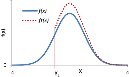
Equations 6(6) $f_T\left(x\right)=\frac{f\left(x\right)}{{\int }_{x_L}^{\mathrm{\infty }}f\left(x\right)dx},x_L<x$(6) and 7(7) $f_T\left(x\right)=\frac{f\left(x\right)}{{\int }_{-\mathrm{\infty }}^{x_U}f\left(x\right)dx},x<x_U$(7) represent the density function of the lower and upper truncated normal distributions. Figure 1 shows the lower truncated normal distribution. The untruncated normal distribution on the same figure is shown by a solid line.

Figure 1. A comparison between lower truncated and none-truncated normal distribution.

(5) $f_T\left(x\right)=\frac{f\left(x\right)}{{\int }_{x_L}^{x_U}f\left(x\right)dx},x_L<x<x_U$(5)

(6) $f_T\left(x\right)=\frac{f\left(x\right)}{{\int }_{x_L}^{\mathrm{\infty }}f\left(x\right)dx},x_L<x$(6)

(7) $f_T\left(x\right)=\frac{f\left(x\right)}{{\int }_{-\mathrm{\infty }}^{x_U}f\left(x\right)dx},x<x_U$(7)

Equation 8(8) ${\mathrm{\varnothing }}_T\left(z\right)=\frac{\mathrm{\varnothing }\left(z\right)}{{\int }_{z_L}^{\mathrm{\infty }}\mathrm{\varnothing }\left(z\right)},z_L<z$(8) represents the density for a lower truncated standard normal distribution ovwe the domain [$z_L$: ∞].

(8) ${\mathrm{\varnothing }}_T\left(z\right)=\frac{\mathrm{\varnothing }\left(z\right)}{{\int }_{z_L}^{\mathrm{\infty }}\mathrm{\varnothing }\left(z\right)},z_L<z$(8)

Equation 9(9) $\mathrm{F}\left(x\right)={\int }_{-\mathrm{\infty }}^x\mathrm{f}\left(\mathrm{t}\right)dt$(9) represents the cumulative density equation for general distributions and enters into the derivation of cumulative density equations for truncated distributions as shown in equations 10(10) $F_T\left(\hspace{0.17em}\right)={\int }_{x_L}^x\frac{f\left(t\right)}{{\int }_{x_L}^{x_U}f\left(t\right)dt}dt,\hspace{0.17em}{x}_L<x<x_U$(10) , 11(11) $F_T\left(x\right)={\int }_{x_L}^x\frac{f\left(t\right)}{{\int }_{x_L}^{\mathrm{\infty }}f\left(t\right)dt}dt,\hspace{0.17em}{x}_L<x$(11) and 12(12) $F_T\left(x\right)={\int }_{-\mathrm{\infty }}^x\frac{f\left(t\right)}{{\int }_{-\mathrm{\infty }}^{x_U}f\left(t\right)dt}dt,\hspace{0.17em}x<x_U$(12) . Equation (10)(10) $F_T\left(\hspace{0.17em}\right)={\int }_{x_L}^x\frac{f\left(t\right)}{{\int }_{x_L}^{x_U}f\left(t\right)dt}dt,\hspace{0.17em}{x}_L<x<x_U$(10) shows the normal distribution cumulative density function that is truncated from both sides, while equations 11(11) $F_T\left(x\right)={\int }_{x_L}^x\frac{f\left(t\right)}{{\int }_{x_L}^{\mathrm{\infty }}f\left(t\right)dt}dt,\hspace{0.17em}{x}_L<x$(11) and 12(12) $F_T\left(x\right)={\int }_{-\mathrm{\infty }}^x\frac{f\left(t\right)}{{\int }_{-\mathrm{\infty }}^{x_U}f\left(t\right)dt}dt,\hspace{0.17em}x<x_U$(12) show the cumulative density of the normal distribution truncated from lower and upper side, respectively. Additionally, Equation 13(13) ${\mathrm{\Phi }}_T\left(x\right)={\int }_{z_L}^z\frac{\mathrm{\varnothing }\left(t\right)}{{\int }_{z_L}^{\mathrm{\infty }}\mathrm{\varnothing }\left(t\right)dt}dt,\hspace{0.17em}{z}_L<z$(13) shows the standard normal distribution cumulative density (i.e., σ = 1, µ = 0) that is truncated from lower side.

(9) $\mathrm{F}\left(x\right)={\int }_{-\mathrm{\infty }}^x\mathrm{f}\left(\mathrm{t}\right)dt$(9)

(10) $F_T\left(\hspace{0.17em}\right)={\int }_{x_L}^x\frac{f\left(t\right)}{{\int }_{x_L}^{x_U}f\left(t\right)dt}dt,\hspace{0.17em}{x}_L<x<x_U$(10)

(11) $F_T\left(x\right)={\int }_{x_L}^x\frac{f\left(t\right)}{{\int }_{x_L}^{\mathrm{\infty }}f\left(t\right)dt}dt,\hspace{0.17em}{x}_L<x$(11)

(12) $F_T\left(x\right)={\int }_{-\mathrm{\infty }}^x\frac{f\left(t\right)}{{\int }_{-\mathrm{\infty }}^{x_U}f\left(t\right)dt}dt,\hspace{0.17em}x<x_U$(12)

(13) ${\mathrm{\Phi }}_T\left(x\right)={\int }_{z_L}^z\frac{\mathrm{\varnothing }\left(t\right)}{{\int }_{z_L}^{\mathrm{\infty }}\mathrm{\varnothing }\left(t\right)dt}dt,\hspace{0.17em}{z}_L<z$(13)

Although these types of equations can be solved through a numerical solution, this type of solution is not practical during industrial and economic applications that need a quick solution. In the same way that the tables of standard normal distributions are developed, many researchers have provided tables for the truncated standard normal distribution, (MM Hamasha, 2017; Khasawneh, Bowling, Kaewkuekool, Cho et al., 2005a, 2005b). However, these tables are not practical and not having a high resolution. Additionally, they do not include all cases, or, in other words, these tables are not complete. The case of Asymmetric double truncation was not considered, for example, due to required huge size table.

In addition, the deviation between the tables and the real values is large. Usually about 0.1 deviation can be found everywhere in the tables. In the following two points, we compare between the table of CDF of standard normal distribution (i.e., z table) and tables for CDF of lower truncated normal distribution: 1) CDF of standard normal distribution is available to a very fine resolution (i.e., 0.001), while the resolution in the tables of lower truncated normal distribution is high. 2) More than a hundred highly accurate and mathematical approximations to the CDF of standard normal distribution are introduced, discussed and implemented. . Examples: Cadwell (1951), Hamaker (1978), Hart (1963), Hoyt (1968), and Bowling et al. (2009).

We concluded that the available CDF tables and other parameters of a lower truncated normal distribution through equations and tables is not an optimum way, and new methods must be found. Moreover, many of the mathematical approximations presented are not as accurate as the model presented in this paper. Later in Section 5, we will compare the presented model with other previous models and show how this model excels in accuracy. In this paper we presented a superfine mathematical model, and the model will be explained in the next section.

3. Proposed model

The model used Zelen and Severo’s normal distribution approximation to approximate aims to approximate CDF of the lower truncated normal distribution. This section is devided into two subsections. In Subsection A, Zelen and Severo’s model is visited. Furthermore, the model accuracy is investigated. Then, in Subsection B, Zelen and Severo’s model is used to derived the paper’s model. The introduced model accuracy is discussed later in Section 5.

3.1. Zelen and severo’s approximation of normal distribution

The Zelen and Severo model is an approximation of the CDF to the normal distribution over the positive z domain, as shown in Equation 14(14) $\mathrm{\Phi }\left(z\right)=1-\left(a_{1}z-a_2{z}^2+a_3{z}^3\right)\frac{e^{-\frac{z^2}{2}}}{\sqrt{2\pi }},\hspace{0.17em}z>0$(14)

(14) $\mathrm{\Phi }\left(z\right)=1-\left(a_{1}z-a_2{z}^2+a_3{z}^3\right)\frac{e^{-\frac{z^2}{2}}}{\sqrt{2\pi }},\hspace{0.17em}z>0$(14)

Where $a_1=\frac{0.4361836}{1+0.33267z}$, $a_2=\frac{0.1201676}{1+0.33267z}$, $a_3=\frac{0.9372986}{1+0.33267z}$

Since the normal distribution is a symmetry about the mean, we can invert the model on the negative z domain by considering the fact of $\left(z\right)=1-\left(-z\right)$, as shown in Equation 15(15) $\mathrm{\Phi }\left(z\right)=\left(a_1{-}_2{z}^2+a_3{z}^3\right)\frac{e^{-\frac{z^2}{2}}}{\sqrt{2\pi }},\hspace{0.17em}z<0$(15) .

(15) $\mathrm{\Phi }\left(z\right)=\left(a_1{-}_2{z}^2+a_3{z}^3\right)\frac{e^{-\frac{z^2}{2}}}{\sqrt{2\pi }},\hspace{0.17em}z<0$(15)

Where $a_1=\frac{0.4361836}{1-0.33267z}$, $a_2=\frac{0.1201676}{1-0.33267z}$, $a_3=\frac{0.9372986}{1-0.33267z}$

The deviation between the presented model and the actual values is defined over the entire z domain (i.e., [-∞: ∞]) to check the accuracy of the model. Figure 2 shows the accuracy of the model on the positive z domain up to z = 4, while Figure 3 shows it on the negative z domain up to z = −4. Each of the two figure’s curves is a reflection of each other about the y = -x axis. Each curve represents a damped wave with 3 peaks at z = 0.5, 1.2 and 2.3, with a deviation value of 0.0000114, 0.0000103, and 0.00001096, respectively. We have to keep in mind that the negative sign of deviation should be ignored. The maximum deviation of the model from the true values over the positive z domain is the second peak from the side z = 0. Similar peaks can be observed on the negative z domain (Figure 3) coming with a similar value of z, but negative, with the same deviation values. As the curve approaches infinity and negative infinity after the third peak, the deviation becomes closer to zero. In other words, the value of the model keeps getting closer to 1 as z increases, and it keeps getting closer to zero as -z decreases. See equation 16(16) $\underset{z\to \mathrm{\infty }}{lim}\left(Equation14\right)=1$(16) and 17(17) $\underset{z\to \mathrm{\infty }}{lim}\left(Equation15\right)=0$(17) .

Figure 2. Deviation in CDF over the domain [0: 4].

Figure 3. Deviation in CDF over the domain [−4: 0].

(16) $\underset{z\to \mathrm{\infty }}{lim}\left(Equation14\right)=1$(16)

(17) $\underset{z\to \mathrm{\infty }}{lim}\left(Equation15\right)=0$(17)

Zelen and Severo’s model in the original form is not include the range of z < 0. However, the fact of Φ(-z) = 1- Φ(z) can be used to apply the model over the negative z range.

In the same way, the deviation versus z-score is drawn the range [−4: 0], as shown in Figure 3.

3.2. Approximation of lower truncated standard normal distribution

The introduced model is developed from Zelen and Severo’s CDF approximation of normal distribution. The first step is to derive this approximation, as addressed in Equation 18(18) $\mathrm{\varnothing }\left(z\right)=\frac{d}{dz}\mathrm{\Phi }\left(z\right)$(18) . Then the derivative result is substituted in Equation 19(19) ${\Phi }_T\left(z\right)={\displaystyle \underset{z_L}{\overset{z}{\int }}\frac{\varnothing \left(z\right)}{{\displaystyle {\int }_{z_L}^{\infty }\varnothing }\left(z\right)dz}}dtz0{\displaystyle \underset{z_L}{\overset{z}{\int }}\frac{\varnothing \left(z\right)}{{\displaystyle {\int }_{z_L}^0\varnothing }\left(z\right)dz+0.5}}dt\text{z}\le 0$(19) and the equation result is gotten

(18) $\mathrm{\varnothing }\left(z\right)=\frac{d}{dz}\mathrm{\Phi }\left(z\right)$(18)

(19) ${\Phi }_T\left(z\right)={\displaystyle \underset{z_L}{\overset{z}{\int }}\frac{\varnothing \left(z\right)}{{\displaystyle {\int }_{z_L}^{\infty }\varnothing }\left(z\right)dz}}dtz0{\displaystyle \underset{z_L}{\overset{z}{\int }}\frac{\varnothing \left(z\right)}{{\displaystyle {\int }_{z_L}^0\varnothing }\left(z\right)dz+0.5}}dt\text{z}\le 0$(19)

As a result of solving previous equations, the approximation model is addressed in Equation 20(20) ${\mathrm{\Phi }}_T\left(z\right)=\frac{1-\left(a_{1}z-a_2{z}^2+a_3{z}^3\right)\frac{e^{-\frac{z^2}{2}}}{\sqrt{2\pi }}-\left(a_4{z}_T-a_5{z_T}^2+a_6{z_T}^3\right)\left(\sqrt{\frac{1}{2\pi }}\right)\frac{e^{-\frac{{z_T}^2}{2}}}{\sqrt{2\pi }}}{1-\left(a_4{z}_T-a_5{z_T}^2+a_6{z_T}^3\right)\left(\sqrt{\frac{1}{2\pi }}\right)\frac{e^{-\frac{{z_T}^2}{2}}}{\sqrt{2\pi }}}\hspace{0.17em}Z>0$(20) and 21(21) ${\mathrm{\Phi }}_T\left(z\right)=\frac{\left(a_{1}z-a_2{z}^2+a_3{z}^3\right)\frac{e^{-\frac{z^2}{2}}}{\sqrt{2\pi }}-\left(a_1{z}_T-a_2{z_T}^2+a_3{z_T}^3\right)\left(\sqrt{\frac{1}{2\pi }}\right)\frac{e^{-\frac{{z_T}^2}{2}}}{\sqrt{2\pi }}}{1-\left(a_1{z}_T-a_2{z_T}^2+a_3{z_T}^3\right)\left(\sqrt{\frac{1}{2\pi }}\right)\frac{e^{-\frac{{z_T}^2}{2}}}{\sqrt{2\pi }}}\hspace{0.17em}Z<0$(21) for the domain positive and negative z, respectively.

(20) ${\mathrm{\Phi }}_T\left(z\right)=\frac{1-\left(a_{1}z-a_2{z}^2+a_3{z}^3\right)\frac{e^{-\frac{z^2}{2}}}{\sqrt{2\pi }}-\left(a_4{z}_T-a_5{z_T}^2+a_6{z_T}^3\right)\left(\sqrt{\frac{1}{2\pi }}\right)\frac{e^{-\frac{{z_T}^2}{2}}}{\sqrt{2\pi }}}{1-\left(a_4{z}_T-a_5{z_T}^2+a_6{z_T}^3\right)\left(\sqrt{\frac{1}{2\pi }}\right)\frac{e^{-\frac{{z_T}^2}{2}}}{\sqrt{2\pi }}}\hspace{0.17em}Z>0$(20)

Where $a_1=\frac{0.4361836}{1+0.33267z}$, $a_2=\frac{0.1201676}{1+0.33267z}$, $a_3=\frac{0.9372986}{1+0.33267z}$, $a_4=\frac{0.4361836}{1-0.33267z}$, $a_5=\frac{0.1201676}{1-0.33267z}$, and$a_6=\frac{0.9372986}{1-0.33267z}$.

(21) ${\mathrm{\Phi }}_T\left(z\right)=\frac{\left(a_{1}z-a_2{z}^2+a_3{z}^3\right)\frac{e^{-\frac{z^2}{2}}}{\sqrt{2\pi }}-\left(a_1{z}_T-a_2{z_T}^2+a_3{z_T}^3\right)\left(\sqrt{\frac{1}{2\pi }}\right)\frac{e^{-\frac{{z_T}^2}{2}}}{\sqrt{2\pi }}}{1-\left(a_1{z}_T-a_2{z_T}^2+a_3{z_T}^3\right)\left(\sqrt{\frac{1}{2\pi }}\right)\frac{e^{-\frac{{z_T}^2}{2}}}{\sqrt{2\pi }}}\hspace{0.17em}Z<0$(21)

Where $a_1=\frac{0.4361836}{1-0.33267z}$, $a_2=\frac{0.1201676}{1-0.33267z}$, $a_3=\frac{0.9372986}{1-0.33267z}$, $a_4=\frac{0.4361836}{1-0.33267z}$, $a_5=\frac{0.1201676}{1-0.33267z}$, and$a_6=\frac{0.9372986}{1-0.33267z}$.

4. Numerical example

Although the main goal of model presented in Equation 20(20) ${\mathrm{\Phi }}_T\left(z\right)=\frac{1-\left(a_{1}z-a_2{z}^2+a_3{z}^3\right)\frac{e^{-\frac{z^2}{2}}}{\sqrt{2\pi }}-\left(a_4{z}_T-a_5{z_T}^2+a_6{z_T}^3\right)\left(\sqrt{\frac{1}{2\pi }}\right)\frac{e^{-\frac{{z_T}^2}{2}}}{\sqrt{2\pi }}}{1-\left(a_4{z}_T-a_5{z_T}^2+a_6{z_T}^3\right)\left(\sqrt{\frac{1}{2\pi }}\right)\frac{e^{-\frac{{z_T}^2}{2}}}{\sqrt{2\pi }}}\hspace{0.17em}Z>0$(20) and Equation 21(21) ${\mathrm{\Phi }}_T\left(z\right)=\frac{\left(a_{1}z-a_2{z}^2+a_3{z}^3\right)\frac{e^{-\frac{z^2}{2}}}{\sqrt{2\pi }}-\left(a_1{z}_T-a_2{z_T}^2+a_3{z_T}^3\right)\left(\sqrt{\frac{1}{2\pi }}\right)\frac{e^{-\frac{{z_T}^2}{2}}}{\sqrt{2\pi }}}{1-\left(a_1{z}_T-a_2{z_T}^2+a_3{z_T}^3\right)\left(\sqrt{\frac{1}{2\pi }}\right)\frac{e^{-\frac{{z_T}^2}{2}}}{\sqrt{2\pi }}}\hspace{0.17em}Z<0$(21) is to enrich the theoretical science, it can be used in different applications. However, the use of these equations to obtain the results is very easy and perhaps easier than other methods and the accuracy and superiority and we will discuss the accuracy in the next section. One of the most common applications that requires analysis of lower truncated normal distribution is the study of the reliability of devices after their use. Technically, reliability is an estimate of how long a device or machine will survive before its final retirement from service. Statistically reliability is equivalent to the complement of CDF (i.e., F(x)), or in other words 1-F (x).

The following is an example. If the life of a particular mechanical tool follows a normal distribution and the average service time for new tools is 10 years with a standard deviation of 2 years. After 4 years of active service for this tool, the reliability engineer comes to analyze its remaining life, and information such as the chance of the tool remaining for another 8 years before retirement can be obtained. There is a chance that a new product will fail before the end of the 4 years, and this chance has already been canceled because the machine we already have had a 4-year maintenance. The probability distribution of the tool at the moment of its existence after 4 of service is a lower truncated normal distribution with a mean of 10 and a standard deviation of 2, and the truncation point is 4. This distribution can be converted into a standard lower truncated normal distribution, and here the truncation point can be calculated with z_L = (4–10)/2 = −3. The time period from the current day to after 8 years represents a period equal to 12 years after adding the usage time of the tool. The point corresponding to six hundred on the truncated ideal distribution can be estimated as follows. z = (12–10)/2 = 1. Simply, we can use Equation 20(20) ${\mathrm{\Phi }}_T\left(z\right)=\frac{1-\left(a_{1}z-a_2{z}^2+a_3{z}^3\right)\frac{e^{-\frac{z^2}{2}}}{\sqrt{2\pi }}-\left(a_4{z}_T-a_5{z_T}^2+a_6{z_T}^3\right)\left(\sqrt{\frac{1}{2\pi }}\right)\frac{e^{-\frac{{z_T}^2}{2}}}{\sqrt{2\pi }}}{1-\left(a_4{z}_T-a_5{z_T}^2+a_6{z_T}^3\right)\left(\sqrt{\frac{1}{2\pi }}\right)\frac{e^{-\frac{{z_T}^2}{2}}}{\sqrt{2\pi }}}\hspace{0.17em}Z>0$(20) (the value of z is greater than 0) and the result is ΦT (1) = 0.840932 and the reliability R(x) = (ie 1- ΦT (1)) as 0.159068. The difference between this value and the actual value does not exceed 0.000002. Table 1 represent the R(x) for the same case based on different models. It is clear that the current model provides a result that is closer to reality than any other model.

Table 1. Reliability Results Using Different Models

	Actual	Current model	Based on Logistic Approximation.	Based on Polya’s Approximation	Based on Hart’s Approximation	Alodat’s Approximation
Reliability, R(x)	0.15887	0.159068	0.155139	0.157009	0.157722	0.0.158958

The model is applicable to complex and repairable equipment without excessive amounts of redundancy, if there is historical data from the manufacturer. Historical data provide sufficient input to develop the desired statistical distribution for the model.

In case we have big data, there are two ways to use the model to deal with this data, as follows. The first method is to program the model using a programming program so that it can deal with big data, but this method is limited to normal data. The second method is to reduce big data and turn it into normal data in the way discussed in (Hamasha et al., 2019; Hamasha et al., 2019; Hamasha et al., 2021; Hamasha et al., 2022).

Although big data usually relies on data sorting and appropriate selection based on certain criteria, truncation of data based on measurements can exist on a scale in a few cases. If each predicate has some attribute that can be measured in some way, and we are interested in omitting the low level of these measures, the result is a truncated distribution on the left side. For example, the data pertains to all Facebook users and the metrics are their age, and the age is normally distributed. Then selecting 50+ people leads us to treat it exactly the same as the example.

5. Analysis of model accuracy

The accuracy of the model is analyzed by defining a function for the deviation of the model values from the true values as presented in Equation 22.

$D\left(z\right)=\mathrm{\Phi }\mathrm{T}{\left(\mathrm{z}\right)}_{Model}-\mathrm{\Phi }\mathrm{T}{\left(\mathrm{z}\right)}_{Real}$ $\left(22\right)$

Figure 4 shows the result of the deviation function for five curves (five truncation points: −4, −3, −2, −1, and 0). It can be seen that there are eight peaks for each curve of the curves representing the truncation points −4 and −3. However, the truncation of the peaks themselves began as the truncation point increased. For example, the truncation point curve representing truncation point −2 has seven peaks after the first peak from the left is cut off. In the same way, the curve representing truncation point −1 has six peaks, and the curve representing truncation point 0 has four peaks. The third peak from the right of all curves has the maximum deviation from all peaks, and it comes at z = 0.5. This peak reached 0.0000115 for the curve representing the truncation point −4, 0.000013 for the curve representing the truncation point −3, 0.000014 for the curve representing the truncation point −2, 0.000011 for the curve representing the truncation point −1, and finally 0.0000023 for the curve representing the truncation point 0.

Figure 4. The model error versus z-score for the four different truncation points.

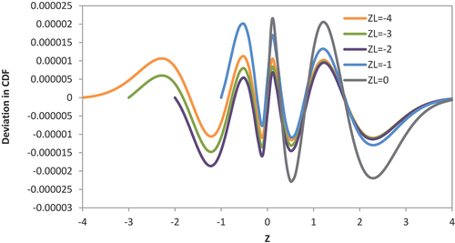
The maximum absolute deviation continued to increase as the truncation point increased from −4 to 0, and is expected to increase further if the truncation point is taken into the positive region. Even the maximum absolute deviation is the highest deviation on the curve, the deviation is still very low and insignificant. In other words, the value of the model is too closed to the actual value and is not felt for applications of applied mathematics.

In order to compare the accuracy of the current model with the previous models, we have adopted the maximum deviation of the curves representing the cutoff points −4, −3, −2, −1, and 0, as shown in Table 2.

Table 2. Maximum absolute deviation of different CDF of lower truncated normal distribution

	Maximum Absolute deviation
	ZL = 0	ZL = −1	ZL = −2	ZL = −3
Introduced	0.0000212	0.00002	0.00000947	0.00000972
Based on Logistic Approximation.	0.018841	0.011012	0.017002	0.012934
Based on Polya’s Approximation	0.006276	0.003856	0.003357	0.003167
Based on Hart’s Approximation	0.0106	0.005727	0.00449	0.00432
Based on Aludaat and Alodat’s Approximation	0.003944	0.002338	0.002534	0.001987

6. Conclusion

In applied mathematics, scientists have attempted to approximate the least truncated normal distribution to enrich the field and open the door to more sophisticated theories and applied analysis in the field. Practically, some practitioners such as reliability engineers used to deal with this kind of distribution. Accordingly, a scientist/engineer usually uses complex software or programs to analyze these statistics. In many cases, a scientist/engineer needs fast results without having to acquire expensive software, and he/she can use the model of this paper. This paper introduces an approximation to the CDF of the cut-off standard low normal distribution. The model provides values that are very close to the true values. The maximum absolute deviation from the real values is 0.0000212 on the region [Z_L: ∞] for any Z_L $\in$ [−4:0].

Disclosure statement

No potential conflict of interest was reported by the author(s).

Additional information

Funding

The authors received no direct funding for this research.

References

- Bouzas, P. R., Aguilera, A. M., & Valderrama, M. J. (2002). Forecasting a class of doubly stochastic poisson processes. Statistical Papers, 43(4), 507. https://doi.org/10.1007/s00362-002-0120-0
- Bowling, S. R., Khasawneh, M. T., Kaewkuekool, S., & Cho, B. R. (2009). A logistic approximation to the cumulative normal distribution. Journal of Industrial Engineering and Management, 2, 114–11. https://doi.org/10.3926/jiem.2009.v2n1.p114-127
- Cadwell, J. H. (1951). The bivariate normal integral. Biometrika, 38(3–4), 475–479. https://doi.org/10.1080/00949659008811236
- Gupta, A. K., & Tracy, D. S. (1976). Recurrence relations for the moments of truncated multinormal distribution. Communications in Statistics - Theory and Methods, 5(9), 855–865. https://doi.org/10.1080/03610927608827402
- Hamaker, H. C. (1978). Approximating the cumulative normal distribution and its inverse. Applied Statistics, 27(1), 76–77. https://doi.org/10.2307/2346231
- Hamasha, M. M. (2017). Practitioner advice: Approximation of the cumulative density of left-sided truncated normal distribution using logistic function and its implementation in microsoft excel. Quality Engineering, 29(2), 322–328. https://doi.org/10.1080/08982112.2016.1196373
- Hamasha, M. M. (2018). Generate random variates using a newly introduced approximation to cumulative density of lower truncated normal distribution for simulation applications. International Journal of Mathematics in Operational Research, 13(3), 265–279. https://doi.org/10.1504/IJMOR.2018.094852
- Hamasha, M. M. (2019). Mathematical approximation of single and double-sided truncated normal distribution using logistic function. International Journal of Industrial Engineering: Theory, Practice and Applications, 26(6), 934–944. https://doi.org/10.23055/ijietap.2019.26.6.3344
- Hamasha, M. M., Ali, H., Hamasha, S., & Ahmed, A. Ultra-fine transformation of data for normality. Heliyon, 8(5), e09370. 2022. https://doi.org/10.1016/j.heliyon.2022.e09370.
- Hamasha, M. M., Ali, H., Hamasha, S., & Ahmed, A. (2021). A mathematical approximation to left-sided truncated normal distribution based on hart’s model. Journal of Applied Engineering Science, 19(4), 1093–1099. https://doi.org/10.5937/jaes0-29895
- Hamasha, M. M., Ali, H., Hamasha, S., & Ahmed, A (2022). An approximation to the inverse of left-sided truncated gaussian cumulative normal density function using to generate random variates for simulation applications. Accepted, Journal of Applied Engineering Science, 20(2). https://doi.org/10.5937/jaes0-35413
- Hart, R. G. A. (1963). Close approximation related to the error function. Mathematics of Computation, 20(96), 600–602. https://doi.org/10.1090/S0025-5718-1966-0203907-1
- Horrace, W. C. (2005). Some results on the multivariate truncated normal distribution. Journal of Multivariate Analysis, 94(1), 209–221. https://doi.org/10.1016/j.jmva.2004.10.007
- Horrace, W. C. (2015). Moments of the truncated normal distribution. Journal of Productivity Analysis, 43(2), 133–138. https://doi.org/10.1007/s11123-013-0381-8
- Hoyt, J. P. A. (1968). Simple approximation to the standard normal probability density function. The American Statistician, 22(3), 25–26. https://doi.org/10.1080/00031305.1968.10480455
- Johnson, N. L., & Kotz, S. (1975). A vector multivariate hazard rate. Journal of Multivariate Analysis, 5(1), 53–66. https://doi.org/10.1016/0047-259X(75)90055-X
- Jolani, S. (2014). An analysis of longitudinal data with nonignorable dropout using the truncated multivariate normal distribution. Journal of Multivariate Analysis, 131, 163–173. https://doi.org/10.1016/j.jmva.2014.06.016
- Khasawneh, M. T., Bowling, S. R., Kaewkuekool, S., & Cho, B. R. (2005a). Tables of a truncated standard normal distribution: A singly truncated case. Quality Engineering, 17(1), 33–50. https://doi.org/10.1081/QEN-200028681
- Khasawneh, M. T., Bowling, S. R., Kaewkuekool, S., & Cho, B. R. (2005b). Tables of a truncated standard normal distribution: A doubly truncated case. Quality Engineering, 17(2), 227–241. https://doi.org/10.1081/QEN-200057321
- McGill, J. I. (1992). The multivariate hazard gradient and moments of the truncated multinormal distribution. Comm Statist Theory Methods, 213053–213060.
- Pearn, W. L., Hung, H. N., Peng, N. F., & Huang, C. Y. (2007). Testing process precision for truncated normal distributions. Microelectronics Reliability, 47(12), 2275–2281. https://doi.org/10.1016/j.microrel.2006.12.001
- Pender, J. (2015). The truncated normal distribution: Applications to queues with impatient customers. Operations Research Letters, 43(1), 40–45. https://doi.org/10.1016/j.orl.2014.10.008
- Rai, B., & Singh, N. (2003). Hazard rate estimation from incomplete and unclean warranty data. Reliability Engineering & System Safety, 81(81), 79–92. https://doi.org/10.1016/S0951-8320(03)00083-8
- Robert, C. P. (1995). Simulation of truncated normal variables. Statistics and Computing, 5(2), 121–125. https://doi.org/10.1007/BF00143942
- Sherif, Y. S. (1982). Inverse truncated normal distribution as a failure model. Reliability Engineering, 3(3), 209–211. https://doi.org/10.1016/0143-8174(82)90030-0
- Smith, M. J. A. (2008). Probabilistic abstract interpretation of imperative programs using truncated normal distributions. Electronic Notes in Theoretical Computer Science, 220(3), 43–59. https://doi.org/10.1016/j.entcs.2008.11.018
- Stein, W. E., Pfaffenberger, R. C., & Mizzi, P. J. (1993). A stochastic dominance comparison of truncated normal distributions. European Journal of Operational Research, 67(2), 259–266. https://doi.org/10.1016/0377-2217(93)90066-V
- Wei, M., Jin, W., & Shen, L. (2012). A platoon dispersion model based on a truncated normal distribution of speed. Journal of Applied Mathematics, 1–13. https://doi.org/10.1155/2012/727839