The m-polar fuzzy ELECTRE-I integrated AHP approach for selection of non-traditional machining processes

Abstract

In the literature, there are a number of decision-making strategies that can be used to choose the best NTM processes. Chen (2014) introduced a novel method to handle fuzzy data that includes multipolar uncertainty, referred to as the m-polar fuzzy set (mFS) approach. The mFS method, along with other multi-criteria decision-making (MCDM) techniques, is a good way to choose between options. An illustration of such a combination is the mFS elimination and choice translating reality-I (ELECTRE-I) . A criteria weight approach is also needed to increase the accuracy of the mFS ELECTRE-I method. The mFS ELECTRE-I method and the analytical hierarchy process (AHP) criteria weight calculation method are combined in the current work. The unique thing about this method is that it can be used to solve both MCDM and MCGDM problems by combining the mFS ELECTRE-I with the AHP criteria weight method. A single-dimensional weight sensitivity analysis is performed to confirm the technique’s stability for different criterion weights for the AHP method on alternative rank performance. The results of the NTM process selection are validated by previous research findings. EDM turned out to be the best way to create machine precise holes on duralumin alloy, and ECM turned out to be the best alternative to generate the surface of revolution in stainless steel. A C++-based soft solution that uses the mFS ELECTRE-I technique to analyze various MCDM and MCGDM problems has been developed. With the soft solution, you can fix problems with selecting the FMS, the robot, and so on.

Keywords:

• m-polar
• ELECTRE-I
• AHP
• TOPSIS
• PROMEETHEE

1. Introduction

The m-polar fuzzy set (mFS) is an extension of the bipolar fuzzy set (Chen et al., 2014).This approach can be used to solve problems with subgroups of criteria. The mFS is mathematically represented by [0,1]^m, where m represents several defined concepts. The mFS algorithm can solve multi-criteria group decision-making (MCGDM) problems. We can solve multi-criteria decision-making (MCDM) and MCGDM problems by combining mFSs with various MCDM techniques. The elimination and choice translating reality-I (ELECTRE-I) method is an outranking method that shows relationships between alternatives using outranking links. The mFS ELECTRE-I method was chosen for the study in this paper. Several researchers are using the mFShybrid approach to solve selection problems in social and scientific domains. The motivation for selecting this study is to integrate the mFS ELECTRE-I algorithm with the analytical hierarchy process (AHP) criteria weight calculation method and introduce a single algorithm that can be used to solve MCDM and MCGDM problems. In this paper, the selection of the NTM process problem is considered in order to implement the mFS ELECTRE-I algorithm. The first section of the article introduces the mFS, ELECTRE-I, and NTM selection. The second section of the literature review describes the various available expert systems for selecting the NTM process. It gives a brief explanation of the ELECTRE method’s evolution over time and the problems it solves, based on literature. The mFS ELECTRE-I integrated AHP methodology is explained step by step in the third section of the paper. In the fourth section, NTM selection example one is solved using the mFS ELECTRE-I integrated AHP algorithm. Following that, in the fifth section, NTM selection example two is solved using the mFS ELECTRE-I integrated AHP algorithm. In section six, the validation of results is explained by comparing the results obtained from the mFS ELECTRE-I integrated AHP algorithm with those obtained from the TOPSIS-AHP method. Finally, in the seventh section, the work’s conclusions are developed.

NTM selection:

One of the most pressing issues that industries face is the selection of NTM processes. The features of NTM processes include obtaining intricate shapes over hard material and performing complicated machining with precision. There are several NTM processes available in practice. Names of NTM processes those are available for machining and NTM processes also have their own set of performance parameters are abrasive jet machining (AJM)(o₁), chemical machining (CHM)(o₂), electrical discharge machining (EDM)(o₃), electrochemical machining (ECM)(o₄), electron beam machining (EBM)(o₅), laser beam machining (LBM) (o₆), ultrasonic machining (USM) (o₇), water jet machining (WJM) (o₈), and wire electrical discharge machining (WEDM) (o₉).

To generate the surface of revolution on stainless steel and machine precision holes on duralumin, we must choose the best process from the options presented above. The parameters considered for a more suitable machining operation are surface finish (SF) (u₁), power requirement (PR) (u₂), material removal rate (MRR) (u₃), cost (C) (u₄), efficiency (E) (u₅), tooling and fixtures (TF) (u₆), tool consumption (TC) (u₇), safety (S) (u₈), work material (M) (u₉), and shape feature (F) (u₁₀).

1.1. Objectives of the work

The objective of this paper is to select a suitable NTM process to generate the surface of revolution on stainless steel and to select a suitable NTM process to machine precision holes on duralumin. Also the mFS ELECTRE-I obtained the outranking relationship between various NTM processes and establish relationships between various NTM processes with a directed graph. The second objective of the work is to perform single dimensional sensitivity analysis in order to find the stability of the mFS ELECTRE-I integrated AHP for varying criteria weights of AHP criteria weight method.

2. Literature review

Because NTM process selection is one of the most important industrial selection problems, the development of NTM process selection scientific/mathematical tools is required, taking into account all machining applications (Chakladar & Chakraborty, 2008). As a result, several authors have created expert systems to select the best NTM process, given a set of input parameters. Table 1 contains a list of such expert systems.

Table 1. Expert system developed by various authors for NTM selection

Sr. No.	Name of expert system	Working on an expert system	Name of author
1	Computer-aided procedure	It uses a 16-digit classification code to rank the NTM process.	(Cogun, 1993)
2	Multi-attribute-based selection procedure	They have employed AHP and TOPSIS to rank feasible NTM processes according to machining application.	(Yurdakul & Çoǧun, 2003)
3	AHP-based expert system	They have considered criteria and sub-criteria priority values related to a particular NTM process.	(Chakraborty & Dey, 2006)
4	Quality function deployment–based expert system	Estimated overall scores from various product and process characteristics and their weights.	(Chakraborty & Dey, 2007)
5	n-tier management information system	Considered parameter selection and optimization in NTM processes using the architecture of MIS.	(Chakrabarti et al., 2007)
6	Combination of TOPSIS and AHP methods	AHP method to calculate weights of parameters and TOPSIS method for ranking alternatives.	(N. D. Chakladar & Chakraborty, 2008)
7	Diagraph-based method	Used digraph method to select the NTM process	(N. Das Chakladar et al., 2009)
8	Web-based, knowledge-based system	They have employed three-tier web architecture to implement user modules to select and expert modules to update the knowledge base.	(Edison Chandrasselan et al., 2008)
9	Two-phase decision model	The first phase uses the Charnes, Cooper, and Rhodes model of data envelopment analysis to select the most efficient process for shape and material. The second phase uses the weighted overall efficiency ranking method to rank alternatives.	(Sadhu & Chakraborty, 2011)
10	Analytical network process–based approach	Analytical network process to consider interdependency and feedback relationship among various criteria and graphic user interface to automate the method.	(Das & Chakraborty, 2011)
11	MOORA method	They have multi-objective optimization based on ratio analysis (MOORA) to choose a process for various machining applications.	(Chakraborty, 2011)
12	Fuzzy-based decision support model	They have used a fuzzy and crisp environment for NTM process selection by assessing the potential of distinct NTM processes.	(Temuçin et al., 2014)
13	PROMETHEE- GAIA method	They have used the PROMETHEE- GAIA method, a visual aid to the decision engineers.	(Karande & Chakraborty, 2012)
14	QFD-based decision-making model	They have created an automated QFD-based decision-making model with the help of Visual BASIC 6.0.	(Prasad & Chakraborty, 2014)
15	Fuzzy axiomatic design principle	They have applied the fuzzy axiomatic design principle to select suitable NTM processes.	(Khandekar & Chakraborty, 2016)
16	Fuzzy AHP and QFD	Fuzzy AHP evaluates the relative importance of various NTM processes and QFD to calculate the overall score of the NTM process.	(Roy et al., 1968)
17	Case-based reasoning approach	They have used a memory model to represent, index, and organize past cases and develop new ones.	(Boral & Chakraborty, 2016)
18	Integrated factor relationship (FARE) and MABAC methods	Used integrated FARE and MABAC methods for NTM process selection.	(Chatterjee et al., 2017)
19	Decision guidance framework	They have designed and developed a decision guidance framework in VISUAL BASICS 6.0 to select suitable NTM processes for intricate and complex shapes.	(Prasad & Chakraborty, 2018)

From the literature, there are the motivations for developing scientific and mathematical tools, which are to assist in decision-making, determine the NTM process based on the machining parameters, automate the decision-making process, create a visual decision aid for the process engineers, and select the NTM process for machining ceramics, hardened tool steels, and titanium materials.

The ELECTRE method was modified by Roy et al. (1968) to become ELECTRE-I (2019; Akram et al., 2019). AHP, TOPSIS, PROMETHEE, and ELECTRE were among the techniques used in MCDM models. Jagtap and Karande (2022) combined the mFS with TOPSIS method for the selection of the NTM process. According to the literature, the ELECTRE family outperforms all other techniques in terms of performance and clarity of decision. In ELECTRE, the “incomparable” preference relation assists decision-makers in comparing alternatives. The concordance and discordance indices quantify relative advantages and disadvantages. To solve real-world problems with incomplete information, many researchers combined fuzzy sets (Zadeh, 1965) with ELECTRE-I. The following is a list of researchers and their work.

Fuzzy ELECTRE was utilised by Rouyendegh and Erkan (2013) to choose academic personnel. Fuzzy group ELECTRE was used by Hatami-Marbini et al. (2013) to assess hazardous waste recycling facilities. Asghari et al. (2010) evaluated mobile payment models using the fuzzy ELECTRE-I approach. The fuzzy ELECTRE-I approach is used by Aytac et al. (2011) to analyse the alternatives for catering companies. The similar methodology is used by Kaya & Kahraman (2011) to assess environmental consequences.

Chen et al. (2014) created the mFS, which is an extension of the bipolar fuzzy set. They solved real-world problems involving multipolar information, multiple agents, multiple objects, multiple attributes, and/or uncertainty. Methods mentioned in Table 2 are incapable of dealing with real-world issues involving multiple attributes and data with multipolar information (Akram et al., 2019). To solve multiple attributes and data as multipolar information, the mFS ELECTRE-I method was developed. They solved real-world problems like locating a diesel plant, locating an airport, and evaluating the performance of a physical sciences instructor. Jagtap (2022) elaborated use of mFS for the selection of non-traditional machining processes. Jagtap et al. (2021) implemented an mFS ELECTRE-I algorithm for industrial robot selection problems. Adeel et al. (2019) created the hesitant mFS ELECTRE-I and m-polar hesitant fuzzy ELECTRE-I methods to solve problems such as site selection for farming and brick selection for construction. Adeel et al. (2019) explained the m-polar fuzzy linguistic ELECTRE-I method to deal with uncertainty that comes with linguistic data. Jagtap & Karande (2021) studied the effect of normalization on the mFS ELECTRE-I algorithm and found that vector normalization is a suitable method for the normalization of decision matrix. The goal of this work is to introduce a suitable weight calculator method in the ELECTRE-I mFS approach. The mFS ELECTRE-I integrated AHP provides a scientific method for calculating parameter weights. The mFS ELECTRE-I integrated AHP approach is applicable for any number of concepts associated with parameters or pole size. The literature and manufacturing case studies examined mFS techniques and compared their findings to those of other researchers. Ranjit & Vimalkumar (2022) integrated the ELECTRE method with the MOORA method, which deals with non-subjective data based on cardinal and most recent data. Jagtap et al. (2022) combined the mFS ELECTRE-I method with Shannon’s entropy weight calculation method, where weight calculation depends on actual experimental data without any expert opinion. The current developed approach deals with subjective data effectively.

Table 2. Decision matrix: performance of various NTM processes to different attributes (N. D. Chakladar & Chakraborty, 2008)

Sr.No.	Parameters
	u1	u2	u3	u4	u5	u6	u7	u8	u9	u10
1	1.0	10.00	500.0	2	4	2	3	1	4	1
2	2.5	0.22	0.8	1	4	2	2	3	4	1
3	2.5	0.24	0.5	1	4	2	2	3	4	1
4	3.0	100.00	400.0	5	2	3	1	3	5	4
5	3.0	0.40	15.0	3	3	2	1	3	5	1
6	3.5	2.70	800.0	3	4	4	4	3	5	1
7	3.5	2.50	600.0	3	4	4	4	3	5	1
8	2.5	0.20	1.6	4	5	2	1	3	4	1
9	2.0	1.40	0.1	3	5	2	1	1	4	1

Though complex in calculation, the ELECTRE family was created to address industrial issues because it provides a clear comparison between two alternatives using outranking relationships. When compared to other methods, the ELECTRE method has the advantage that it compares each alternative with all other alternatives that are available in the outranking relation, making it more useful than the other MCDM techniques.

2.1. Problems from literature

In the study by N. D. Chakladar & Chakraborty (2008), the generation of the surface of a revolution shape on stainless steel and the efficient machine of precision holes on duralumin were both considered. Beneficial, non-beneficial, quantitative, and qualitative parameters are classified. Furthermore, they organised data as cardinal data.

In the given NTM selection problem, the criteria are divided into beneficial, non-beneficial, qualitative, and quantitative. The beneficial criteria are material removal rate (MRR), efficiency (E), safety (S), work material (M), and shape feature (F). The non-beneficial criteria are tolerance and surface finish (TSF), power requirement (PR), cost (C), tooling and fixtures (TF), and tool consumption (TC). High values are preferred for beneficial parameters, while low values are preferred for non-beneficial parameters. The qualitative criteria are cost (C), efficiency (E), tooling and fixtures (TF), tool consumption (TC), safety (S), work material (M), and shape feature (F). The quantitative criteria are tolerance and surface finish (TSF), power requirement (PR), and material removal rate (MRR). Quantitative parameters have numerical values, whereas qualitative parameters are represented by rank value judgment on a scale of 1–5 (1–low, 3–moderate, and 5–high). To generate a revolution in stainless steel and create holes in duralumin, we must choose an appropriate NTM process.

The mFS is an unique strategy developed by Chen (2014) to tackle the MCGDM problem. When used alone, the mFS has some limitations. The most well-known aspect of the ELECTRE-I technique is the outranking connection between choices. We can compare two alternatives from the set of alternatives using the concordance and discordance indices. The mFS and ELECTRE-I can be utilised as the decision-making tools for both MCDM and MCGDM scenarios. The mFS ELECTRE-I with AHP criteria weight computations considerably improve the accuracy of the findings. Prior researchers employed the mFS ELECTRE-I methodology directly using criteria weight since it is totally reliant on expert opinion. The mFS ELECTRE-I approach is highly suited for MCGDM problems in society, engineering, and business. In the current study, the MCDM problem is used to show the effectiveness of the mFS ELECTRE-I method in solving the industrial selection problem. The decision support systems created by other researchers are intended for a specific use; however, the soft solution developed in this work is so reliable that it can be used for different industrial applications like choosing an FMS, cutting fluid, or robot, among others.

3. Methodology

This paper will modify the mFS ELECTRE-I algorithm by introducing the AHP method of criteria weight for weight calculations. The mFS is used as the algorithm’s input. The algorithm can be used to evaluate both actual and imprecise data. The mFS ELECTRE-I integrated AHP method is explained in detail below:

1. Let O= {o₁,o₂,o₃, … … … o_n} set of options (alternatives) available with U= {u₁,u₂,u₃, … … … u_n} set of criteria.

2. The decision matrix can be represented as a value of alternative to criteria with the help of

S= (s_ij) = {s_ij¹,s_ij²,s_ij³, … … .s_ij^m}.

• (3) A normalized decision matrix is formulated using the vector normalization method, as shown in equation (1)(1) $\mathit{N}=\frac{{\mathit{s}}_{\mathit{ij}}}{\sqrt{{\sum }_{i=1}^m{s}_{ij}^2}}$(1) .

(1) $\mathit{N}=\frac{{\mathit{s}}_{\mathit{ij}}}{\sqrt{{\sum }_{i=1}^m{s}_{ij}^2}}$(1)

• (4) We are using the AHP method to calculate the weights of the criteria. Let D represent the pairwise comparison matrix. In the AHP method, the relative importance of attributes can be estimated using a pairwise matrix. A pairwise comparison matrix is constructed using Saaty’s nine-point scale. The nine-point scale is divided into two groups of numbers as the importance of the criterion increases from left to right (1, 3, 5, 7, 9). In contrast, the second set (2, 4, 6, 8) demonstrates an intermediate preference for the criterion. The principle of reflexivity is used to compare one measure to another. The first set is used for the pairwise comparison matrix. The diagonal elements of the pairwise comparison matrix are self-compared and have the same value.

$\mathit{D}=\left[\begin{array}{cccc}1& {\mathrm{d}}_{12}& \cdots & d_{1\mathrm{n}}\\ {\mathrm{d}}_{21}& d_{22}& \dots & {\mathrm{d}}_{2\mathrm{n}}\\ ⋮& \dots & \ddots & ⋮\\ {\mathrm{d}}_{\mathrm{n}1}& {\mathrm{d}}_{\mathrm{n}2}& \cdots & 1\end{array}\right]$

The left and right sides of the diagonal matrix represent the strength of relative importance of one attribute concerning the other corresponding attribute. The normalization of the geometric mean is used to evaluate the importance degree of the attributes.

And let w_i denote the importance of i^th attributes, w_i can be evaluated with equation (2)(2) ${\text{w}}_{\text{\hspace{0.05em}i}}\text{=}\frac{{(\underset{\text{\hspace{0.05em}j=1}}{\overset{}{{{\displaystyle \prod }}^n}}{\text{d}}_{\text{\hspace{0.05em}ij}})}^{\text{\hspace{0.05em}1/n}}}{\underset{\text{\hspace{0.05em}i=1}}{\overset{}{{{\displaystyle \sum }}^n}}{(\underset{\text{\hspace{0.05em}j=1}}{\overset{}{{{\displaystyle \prod }}^n}}{\text{d}}_{\text{\hspace{0.05em}ij}})}^{\text{\hspace{0.05em}1/n}}}\text{i},\text{j=1},\text{2},\text{3}\dots \text{n}$(2) .

(2) ${\text{w}}_{\text{\hspace{0.05em}i}}\text{=}\frac{{(\underset{\text{\hspace{0.05em}j=1}}{\overset{}{{{\displaystyle \prod }}^n}}{\text{d}}_{\text{\hspace{0.05em}ij}})}^{\text{\hspace{0.05em}1/n}}}{\underset{\text{\hspace{0.05em}i=1}}{\overset{}{{{\displaystyle \sum }}^n}}{(\underset{\text{\hspace{0.05em}j=1}}{\overset{}{{{\displaystyle \prod }}^n}}{\text{d}}_{\text{\hspace{0.05em}ij}})}^{\text{\hspace{0.05em}1/n}}}\text{i},\text{j=1},\text{2},\text{3}\dots \text{n}$(2)

The summation of all the criterion weights will be one, represented by equation (3).

(3) $1={\sum }_{\mathrm{i}=1}^{\mathrm{n}}{\mathrm{w}}_{\mathrm{i}}$(3)

A consistency ratio is introduced to verify the pairwise comparison matrix’s output. The value of the consistency ratio shows it is acceptable. Let’s E represent the column vector having n-dimensions, which describes the sum of the weighted values for the importance degree of the attributes. E matrix can be mathematically expressed in equation (4)(4) $\mathrm{E}=\mathrm{D}{\mathrm{W}}^{\mathrm{T}}$(4) .

(4) $\mathrm{E}=\mathrm{D}{\mathrm{W}}^{\mathrm{T}}$(4)

Where DW^T = $\left[\begin{array}{cccc}1& {\mathrm{d}}_{12}& \cdots & {\mathrm{d}}_{1\mathrm{n}}\\ {\mathrm{d}}_{21}& {\mathrm{d}}_{22}& \dots & {\mathrm{d}}_{2\mathrm{n}}\\ ⋮& \dots & \ddots & ⋮\\ {\mathrm{d}}_{\mathrm{n}1}& {\mathrm{d}}_{\mathrm{n}2}& \cdots & 1\end{array}\right]\left[\begin{array}{cccc}{\mathrm{w}}_1,& {\mathrm{w}}_2,& \dots .& {\mathrm{w}}_{\mathrm{n}}\end{array}\right]$ =$\left[\begin{array}{c}{\mathrm{E}}_1\\ {\mathrm{E}}_2\\ \dots \\ {\mathrm{E}}_{\mathrm{n}}\end{array}\right]$ (5)

Saaty suggested using the Eigen value (λ_max) to avoid inconsistency; and λ_max is used to evaluate the effectiveness of judgment. The value of λ_max closure to n shows more consistent evaluation. λ_max is formulated as shown in equation (6):

${\mathit{\lambda }}_{\max }=\frac{{\sum }_{\mathrm{i}=1}^n{\mathrm{E}}_{\mathrm{c}}}{\mathrm{n}}$ Where i =1,2,3, … … n.(6)

With λ_max consistency index (CI) can be defined as shown in equation (7):(7) $\mathrm{CI}=\frac{{\mathit{\lambda }}_{\max }-\mathrm{n}}{\mathrm{n}-1}$(7)

(7) $\mathrm{CI}=\frac{{\mathit{\lambda }}_{\max }-\mathrm{n}}{\mathrm{n}-1}$(7)

For CI = 0, the comparison matrix is perfectly consistent.

Furthermore, the consistency ratio (CR) is used for the consistency check, as shown in equation (8)(8) $\mathrm{CR}=\frac{\mathrm{CI}}{\mathrm{RI}}$(8) .

(8) $\mathrm{CR}=\frac{\mathrm{CI}}{\mathrm{RI}}$(8)

Where RI is a random index obtained from different orders of pairwise comparison matrices.

For CR< 0.10, degrees of attributes are reasonable.

• (5) Applying weight to the m-polar decision matrix, B=(b_ij) is formed. Finally, B is a weighted normalized matrix constructed by multiplying each column of the u_ij by w_j as shown in equation (9)(9) $\mathit{B}=\left(b_{\mathit{ij}}\right)=\left({{\mathit{b}}_{\mathit{ij}}}^1,{{\mathit{b}}_{\mathit{ij}}}^2,{{\mathit{b}}_{\mathit{ij}}}^3,\dots .\dots \mathit{\hspace{0.17em}}.{{\mathit{b}}_{\mathit{ij}}}^{\mathit{m}}\right)\mathrm{here}{b}_{\mathit{ij}}=w_j{s}_{\mathit{ij}}$(9) .

(9) $\mathit{B}=\left(b_{\mathit{ij}}\right)=\left({{\mathit{b}}_{\mathit{ij}}}^1,{{\mathit{b}}_{\mathit{ij}}}^2,{{\mathit{b}}_{\mathit{ij}}}^3,\dots .\dots \mathit{\hspace{0.17em}}.{{\mathit{b}}_{\mathit{ij}}}^{\mathit{m}}\right)\mathrm{here}{b}_{\mathit{ij}}=w_j{s}_{\mathit{ij}}$(9)

• (6) The following condition obtains concordance sets. A weighted normalized matrix is further evaluated to compare the elements to see the column-wise dominance of one part over the other component with the value obtained y_ij. All such dominant elements are numbered in the concordance set. The concordance set can be mathematically shown with equation (10)(10) $\mathrm{Here}{\mathrm{y}}_{\mathrm{ij}}={{\mathrm{b}}_{\mathrm{ij}}}^1+\mathit{\hspace{0.17em}}{{\mathrm{b}}_{\mathrm{ij}}}^2+{{\mathrm{b}}_{\mathrm{ij}}}^3\dots .\dots \mathit{\hspace{0.17em}}.+\mathit{\hspace{0.17em}}{{\mathrm{b}}_{\mathrm{ij}}}^{\mathrm{m}}$(10) .

$C_{\mathit{pq}}=\left\{1\le \mathit{j}\le \mathit{u}:y_{\mathit{pj}}\ge \mathit{\hspace{0.17em}}{y}_{\mathit{qj}},\mathit{p}\ne \mathit{q};\mathit{p},\mathit{q}=1,2,\dots .\dots \dots \mathit{n}\right\}$

(10) $\mathrm{Here}{\mathrm{y}}_{\mathrm{ij}}={{\mathrm{b}}_{\mathrm{ij}}}^1+\mathit{\hspace{0.17em}}{{\mathrm{b}}_{\mathrm{ij}}}^2+{{\mathrm{b}}_{\mathrm{ij}}}^3\dots .\dots \mathit{\hspace{0.17em}}.+\mathit{\hspace{0.17em}}{{\mathrm{b}}_{\mathrm{ij}}}^{\mathrm{m}}$(10)

• (7) The following condition obtains discordance sets. A weighted normalized matrix is further evaluated for the element (criterion) comparison to see the column-wise most negligible value of one element over the other elements for the value obtained y_ij. Then, all such least value elements (criterion) are numbered in a discordance set. The discordance set can be mathematically shown with equation (11)(11) $\mathrm{Here}{y}_{\mathit{ij}}={{\mathit{b}}_{\mathit{ij}}}^1+\mathit{\hspace{0.17em}}{{\mathit{b}}_{\mathit{ij}}}^2+{{\mathit{b}}_{\mathit{ij}}}^3\dots .\dots \mathit{\hspace{0.17em}}.+\mathit{\hspace{0.17em}}{{\mathit{b}}_{\mathit{ij}}}^{\mathit{m}}$(11) .

$A_{\mathit{pq}}=\left\{1\le \mathit{\hspace{0.17em}}\mathit{j}\le \mathit{u}:y_{\mathit{pj}}\le \mathit{\hspace{0.17em}}{y}_{\mathit{qj}},\mathit{p}\ne \mathit{q};\mathit{p},\mathit{q}=1,2,\dots .\dots \dots \mathit{n}\right\}$

(11) $\mathrm{Here}{y}_{\mathit{ij}}={{\mathit{b}}_{\mathit{ij}}}^1+\mathit{\hspace{0.17em}}{{\mathit{b}}_{\mathit{ij}}}^2+{{\mathit{b}}_{\mathit{ij}}}^3\dots .\dots \mathit{\hspace{0.17em}}.+\mathit{\hspace{0.17em}}{{\mathit{b}}_{\mathit{ij}}}^{\mathit{m}}$(11)

• (8) The concordance value of indices is formed by adding weights of all such elements (criterion) weights from the concordance set of each element and mathematically represented as shown in equation (12).

c_pq =${\sum }_{\mathrm{j}\in {\mathrm{k}}_{\mathrm{pq}}}{\mathrm{w}}_{\mathrm{j}}$, for all p,q.(12)

• (9) The concordance matrix K can be obtained with all the concordance indices formed with equation (12).

$\mathit{C}=\left(\begin{array}{cccc}-& {\mathrm{c}}_{12}& \mathit{\hspace{0.17em}}{\mathrm{c}}_{13}& {\mathrm{c}}_{1\mathrm{n}}\\ {\mathrm{c}}_{21}& -& ..& {\mathrm{c}}_{2\mathrm{n}}\\ :& :& :& :\\ {\mathrm{c}}_{\mathrm{n}1}& {\mathrm{c}}_{\mathrm{n}2}& \cdots & -\end{array}\right)$

• (10) Discordance indices values are evaluated with the help of the following equation (13).

$a_{\mathit{pq}}=\frac{\mathrm{ma}{\mathrm{x}}_{\mathrm{j}\in {\mathrm{a}}_{\mathrm{pq}}}\sqrt{\frac{1}{\mathrm{m}}\left[{\left({{\mathit{b}}^1}_{\mathrm{pj}}-{{\mathrm{b}}^1}_{\mathrm{qj}}\right)}^2+{\left({{\mathrm{b}}^2}_{\mathrm{pj}}-{{\mathrm{b}}^2}_{\mathrm{qj}}\right)}^2+\dots +{\left({{\mathrm{b}}^{\mathrm{m}}}_{\mathrm{pj}}-{{\mathrm{b}}^{\mathrm{m}}}_{\mathrm{qj}}\right)}^2\right]}}{\mathrm{ma}{\mathrm{x}}_{\mathrm{j}}\sqrt{\frac{1}{\mathrm{m}}\left[{\left({{\mathrm{b}}^1}_{\mathrm{pj}}-{{\mathrm{b}}^1}_{\mathrm{qj}}\right)}^2+{\left({{\mathrm{b}}^2}_{\mathrm{pj}}-{{\mathrm{b}}^2}_{\mathrm{qj}}\right)}^2+\dots +{\left({{\mathrm{b}}^{\mathrm{m}}}_{\mathrm{pj}}-{{\mathrm{b}}^{\mathrm{m}}}_{\mathrm{qj}}\right)}^2\right]}}$ for all p,q(13)

• (11) The discordance matrix A can be obtained with all the discordance indices formed with equation (13).

$\mathit{A}=\left(\begin{array}{cccc}-& {\mathrm{a}}_{12}& {\mathrm{a}}_{13}& {\mathrm{a}}_{1\mathrm{n}}\\ {\mathrm{a}}_{21}& -& ..& a_{2\mathrm{n}}\\ :& :& :& :\\ {\mathrm{a}}_{\mathrm{n}1}& {\mathrm{a}}_{\mathrm{n}2}& \cdots & -\end{array}\right)$

• (12) Levels of concordance (k) and discordance (v) can be formulated as shown in equations (14) and (15).

(14) $\acute{c}=\frac{1}{\mathit{n}(\mathit{n}-1)}{\sum }_{\begin{array}{c}p=1\\ p\ne q\end{array}}^n{\sum }_{\begin{array}{c}q=1\\ q\ne p\end{array}}^n{c}_{\mathit{pq}}$(14)

(15) $\acute{a}=\frac{1}{\mathit{n}(\mathit{n}-1)}{\sum }_{\begin{array}{c}p=1\\ p\ne q\end{array}}^n{\sum }_{\begin{array}{c}q=1\\ q\ne p\end{array}}^n{a}_{\mathit{pq}}$(15)

• (13) From concordance and discordance levels, we can form the concordance dominance matrix and discordance dominance matrix. Equations (16) and (17(17) ${\text{e}}_{\text{\hspace{0.05em}pq}}\text{=1},{\text{a}}_{\text{\hspace{0.05em}pq}}\ge \acute{a}\text{ 0},{\text{a}}_{\text{\hspace{0.05em}pq}}\le \acute{a}$(17) ) show the if-and-then conditions to obtain the concordance matrix L and discordance matrix E elements.

$\mathit{L}=\left(\begin{array}{cccc}-& {\mathrm{l}}_{12}& \mathit{\hspace{0.17em}}{\mathrm{l}}_{13}& {\mathrm{l}}_{1\mathrm{n}}\\ {\mathrm{l}}_{21}& -& ..& {\mathrm{l}}_{2\mathrm{n}}\\ :& :& :& :\\ {\mathrm{l}}_{\mathrm{n}1}& {\mathrm{l}}_{\mathrm{n}2}& \cdots & -\end{array}\right)$

Here

(16) $[\mathit{\$\$}{l}_{\mathit{pq}}=1,c_{\mathit{pq}}\ge \acute{c}0,c_{\mathit{pq}}\le \acute{c}$(16)

$\mathit{E}=\left(\begin{array}{cccc}-& {\mathrm{e}}_{12}& \mathit{\hspace{0.17em}}{\mathrm{e}}_{13}& {\mathrm{e}}_{1\mathrm{n}}\\ {\mathrm{e}}_{21}& -& ..& {\mathrm{e}}_{2\mathrm{n}}\\ :& :& :& :\\ {\mathrm{e}}_{\mathrm{n}1}& {\mathrm{e}}_{\mathrm{n}2}& \cdots & -\end{array}\right)$

Here

(17) ${\text{e}}_{\text{\hspace{0.05em}pq}}\text{=1},{\text{a}}_{\text{\hspace{0.05em}pq}}\ge \acute{a}\text{ 0},{\text{a}}_{\text{\hspace{0.05em}pq}}\le \acute{a}$(17)

• (14) To obtain the aggregate dominance matrix F, perform a point-to-point multiplication of L and E matrix values

$\mathit{F}=\left(\begin{array}{cccc}-& {\mathrm{f}}_{12}& \mathit{\hspace{0.17em}}{\mathrm{f}}_{13}& {\mathrm{f}}_{1\mathrm{n}}\\ {\mathrm{f}}_{21}& -& ..& {\mathrm{f}}_{2\mathrm{n}}\\ :& :& :& :\\ {\mathrm{f}}_{\mathrm{n}1}& {\mathrm{f}}_{\mathrm{n}2}& \cdots & -\end{array}\right)$

Above 14en steps are to be followed for solving the selection problem with the mFS ELECTRE-I integrated AHP method. Matrices L, E, and F are used for outranking relations between alternatives.

3.1. Sensitivity analysis

Sensitivity analysis is a procedure used to look into how changing input can affect output for the MCDM process. There are other types of sensitivity analysis, but the two most common types are single-dimensional weight sensitivity analysis (SDWSA) and high-dimensional weight sensitivity analysis (HDWSA). While HDWSA uses the performance score to determine the most important criteria weight, SDWSA uses a weight additive constraint. To determine the range of criteria weight stability, SDWSA is now being used. Due to the lack of a performance score for the mFS ELECTRE-I method, HDWSA cannot be performed. The local and global stability range for the weight of the criteria is examined in SDWSA.

We must take into account the variable with the highest criteria weight when doing SDWSA. Utilizing a weight additive constraint, the weight of the chosen variable criteria should be increased from zero to maximum. For SDWSA, you can use the following formula:

$\mathrm{W}=\left[{\mathrm{W}}_{\max }+\left(\mathrm{n}-1\right)\times {\mathrm{W}}_{\min }\right]$

Where W is the varying criteria weight of maximum criteria weight, W_max is the maximum criteria weight, and W_min is the minimum criteria weight.

4. Example-I: selection of NTM process for the surface of revolution on stainless steel

N. D. Chakladar & Chakraborty (2008) for the surface of revolution on stainless steel problem chose nine different NTM processes with ten parameters. The decision matrix for the same case is given in Table 2. TSF,PR, and MRR parameters have actual values (quantitative), while the remaining parameters are shown as qualitative values with the help of a five-point scale.

Table 3 shows the normalised decision matrix obtained with the vector normalisation method from Table 2.

Table 3. Normalised decision matrix

Sr.	Parameters
	u1	u2	u3	u4	u5	u6	u7	u8	u9	u10
o1	0.1229	0.0994	0.4210	0.2195	0.3345	0.2481	0.4121	0.1240	0.2981	0.2041
o2	0.3071	0.0022	0.0007	0.1098	0.3345	0.2481	0.2747	0.3721	0.2981	0.2041
o3	0.3071	0.0024	0.0004	0.1098	0.3345	0.2481	0.2747	0.3721	0.2981	0.2041
o4	0.3686	0.9943	0.3368	0.5488	0.1672	0.3721	0.1374	0.3721	0.3727	0.8165
o5	0.3686	0.0040	0.0126	0.3293	0.2509	0.2481	0.1374	0.3721	0.3727	0.2041
o6	0.4300	0.0268	0.6737	0.3293	0.3345	0.4961	0.5494	0.3721	0.3727	0.2041
o7	0.4300	0.0249	0.5053	0.3293	0.3345	0.4961	0.5494	0.3721	0.3727	0.2041
o8	0.3071	0.0020	0.0013	0.4391	0.4181	0.2481	0.1374	0.3721	0.2981	0.2041
o9	0.2457	0.0139	0.0001	0.3293	0.4181	0.2481	0.1374	0.1240	0.2981	0.2041

Finally, a nine-point scale gives a pairwise comparison for parameters in Table 4. The significance of scale values is elaborated as 1—equally important, 3—weakly important, 5—strongly important, 7—very strongly important, and 9—absolutely important, while 2, 4, 6, and 8 show intermediate preference value.

Table 4. Pairwise comparison matrix

	u1	u2	u3	u4	u5	u6	u7	u8	u9	u10
u1	1	2	1/3	1/2	3	4	5	6	1/5	1/4
u2	1/2	1	1/3	1/2	2	3	4	5	1/5	1/4
u3	3	3	1	2	5	6	7	8	1/2	1/3
u4	2	2	1/2	1	4	5	6	7	1/4	1/3
u5	1/3	1/2	1/5	1/4	1	2	3	4	1/7	1/6
u6	1/4	1/3	1/6	1/5	1/2	1	2	3	1/8	1/7
u7	1/5	1/4	1/7	1/6	1/3	1/2	1	2	1/9	1/8
u8	1/6	1/5	1/8	1/7	1/4	1/3	1/2	1	1/9	1/9
u9	5	5	2	4	7	8	9	9	1	2
u10	4	4	3	3	6	7	8	9	1/2	1

Equation (2)(2) ${\text{w}}_{\text{\hspace{0.05em}i}}\text{=}\frac{{(\underset{\text{\hspace{0.05em}j=1}}{\overset{}{{{\displaystyle \prod }}^n}}{\text{d}}_{\text{\hspace{0.05em}ij}})}^{\text{\hspace{0.05em}1/n}}}{\underset{\text{\hspace{0.05em}i=1}}{\overset{}{{{\displaystyle \sum }}^n}}{(\underset{\text{\hspace{0.05em}j=1}}{\overset{}{{{\displaystyle \prod }}^n}}{\text{d}}_{\text{\hspace{0.05em}ij}})}^{\text{\hspace{0.05em}1/n}}}\text{i},\text{j=1},\text{2},\text{3}\dots \text{n}$(2) is used to calculate the weights of the criterion. For the example-I, we got values of criterion weights as follows:

W_TSF = 0.0783, W_PR = 0.0611, W_MRR = 0.1535, W_C = 0.1073, W_E = 0.0383, W_TF = 0.0271, W_TC = 0.0195, W_S = 0.0146, W_M = 0.2766, W_F = 0.2237.

Equations (6(8) $\mathrm{CR}=\frac{\mathrm{CI}}{\mathrm{RI}}$(8) ) and (8(8) $\mathrm{CR}=\frac{\mathrm{CI}}{\mathrm{RI}}$(8) ) are used for the evaluation of the maximum Eigen value (λ_max) and consistency ratio (CR). For the pairwise comparison matrix shown in Table 5 and 6, λ_max = 10.5749 and CR = 0.0403. It shows consistency, as this value is less than 0.10. It is without any bias.

Table 5. Weighted normalised matrix

Sr.	Parameters
	u1	u2	u3	u4	u5	u6	u7	u8	u9	u10
o1	0.0096	0.0061	0.0646	0.0236	0.0128	0.0067	0.0080	0.0018	0.0825	0.0457
o2	0.0240	0.0001	0.0001	0.0118	0.0128	0.0067	0.0054	0.0054	0.0825	0.0457
o3	0.0240	0.0001	0.0001	0.0118	0.0128	0.0067	0.0054	0.0054	0.0825	0.0457
o4	0.0289	0.0607	0.0517	0.0589	0.0064	0.0101	0.0027	0.0054	0.1031	0.1827
o5	0.0289	0.0002	0.0019	0.0353	0.0096	0.0067	0.0027	0.0054	0.1031	0.0457
o6	0.0337	0.0016	0.1034	0.0353	0.0128	0.0134	0.0107	0.0054	0.1031	0.0457
o7	0.0337	0.0015	0.0776	0.0353	0.0128	0.0134	0.0107	0.0054	0.1031	0.0457
o8	0.0240	0.0001	0.0002	0.0471	0.0160	0.0067	0.0027	0.0054	0.0825	0.0457
o9	0.0192	0.0009	0.0001	0.0353	0.0160	0.0067	0.0027	0.0018	0.0825	0.0457

Table 6. Concordance set

j	1	2	3	4	5	6	7	8	9
C1j	-	{2,3,4,5,6,7,9,10}	{2,3,4,5,6,7,9,10}	{3,5,7}	{2,3,5,6,7,10}	{2,5,10}	{2,5,10}	{2,3,6,7,9,10}	{2,3,6,7,8,9,10}
C2j	{1,5,6,8,9,10}	-	{1,3,4,5,6,7,8,9,10}	{5,7,8}	{5,6,7,8,10}	{5,8,10}	{5,8,10}	{1,2,6,7,8,9,10}	{1,3,6,7,8,9,10}
C3j	{1,5,6,8,9,10}	{1,2,4,5,6,7,8,9,10}	-	{5,7,8}	{5,6,7,8,10}	{5,8,10}	{5,8,10}	{1,2,6,7,8,9,10}	{1,3,6,7,8,9,10}
C4j	{1,2,4,6,8,9,10}	{1,2,3,4,6,8,9,10}	{1,2,3,4,6,8,9,10}	-	{1,2,3,4,6,7,8,9,10}	{2,4,8,9,10}	{2,4,8,9,10}	{1,2,3,4,6,7,8,9,10}	{1,2,3,4,6,7,8,9,10}
C5j	{1,4,6,8,9,10}	{1,2,3,4,6,8,9,10}	{1,2,3,4,6,8,9,10}	{1,5,7,8,9}	-	{4,8,9,10}	{4,8,9,10}	{1,2,3,6,7,8,9,10}	{1,3,4,6,7,8,9,10}
C6j	{1,3,4,5,6,7,8,9,10}	{1,2,3,4,5,6,7,8,9,10}	{1,2,3,4,5,6,7,8,9,10}	{1,3,5,6,7,8,9}	{1,2,3,4,5,6,7,8,9,10}	-	{1,2,3,4,5,6,7,8,9,10}	{1,2,3,6,7,8,9,10}	{1,2,3,4,6,7,8,9,10}
C7j	{1,3,4,5,6,7,8,9,10}	{1,2,3,4,5,6,7,8,9,10}	{1,2,3,4,5,6,7,8,9,10}	{1,3,5,6,7,8,9}	{1,2,3,4,5,6,7,8,9,10}	{1,4,5,6,7,8,9,10}	-	{1,2,3,6,7,8,9,10}	{1,2,3,4,6,7,8,9,10}
C8j	{1,4,5,6,8,9,10}	{1,3,4,5,6,8,9,10}	{1,3,4,5,6,8,9,10}	{5,7,8}	{4,5,6,7,8,10}	{4,5,8,10}	{4,5,8,10}	-	{1,3,4,5,6,7,8,9,10}
C9j	{1,4,5,6,8,9,10}	{2,4,5,6,9,10}	{2,4,5,6,9,10}	{5,7}	{2,4,5,6,7,10}	{4,5,10}	{4,5,10}	{2,5,6,7,9,10}	-

Table 5 shows the weighted normalised matrix.

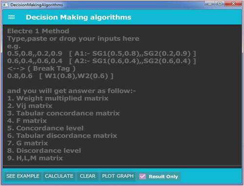
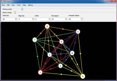
A decision system is developed using C++ software to select the suitable NTM process in industry. It is simple in use. A decision maker from the industry can use developed solution as shown in Figure 1 to solve the problem related to the selection of NTM process.

Figure 1. Console of the soft solution with instructions given for the input and output expected after the implementation of the mFS ELECTRE-I integrated approach.

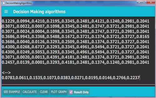
The decision system is developed in the robust way such that it can handle other decision problems from the industry by giving just input of decision matrix related to the problem with AHP weight. Figure 2 represents actual input given in the example-I in the form of normalized decision matrix. One can use direct decision matrix as input; the normalised decision matrix gave better rank performance as compared with the decision matrix without normalization.

Figure 2. Actual input is given to the console in the form of normalised decision matrix and weight obtained from the AHP method.

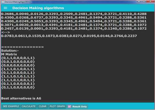
There are tabs available at the bottom task bar to perform different functions of the algorithm. “SEE EXAMPLE” tab will show sample examples to guide users to give input. “CALCULATE” tab will be used for obtaining detailed solution of the input given to the console. Appendix-I given at the end of the paper shows complete results obtained from the decision system. If we select “Result Only” selection box, summary results for the given problem comes on the screen. Figure 3 presents summary results for example-I. “CLEAR” tab on the task bar will clear console for the next problem.

Figure 3. Results obtained for the given input data.

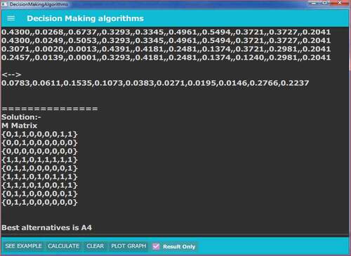
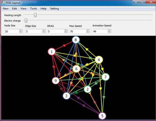
“PLOT GRAPH” on the console will plot a graph for the given input. Summary of the results obtained in Figure 3 can be used for deciding rank of alternatives. And the digraph plotted as shown in Figure 4 explains pictorial presentation of the dominance of one alternative over the other alternative.

Figure 4. Directed graph is plotted on the console with C++ code for example-I.

Equation (10)(10) $\mathrm{Here}{\mathrm{y}}_{\mathrm{ij}}={{\mathrm{b}}_{\mathrm{ij}}}^1+\mathit{\hspace{0.17em}}{{\mathrm{b}}_{\mathrm{ij}}}^2+{{\mathrm{b}}_{\mathrm{ij}}}^3\dots .\dots \mathit{\hspace{0.17em}}.+\mathit{\hspace{0.17em}}{{\mathrm{b}}_{\mathrm{ij}}}^{\mathrm{m}}$(10) and equation (11)(11) $\mathrm{Here}{y}_{\mathit{ij}}={{\mathit{b}}_{\mathit{ij}}}^1+\mathit{\hspace{0.17em}}{{\mathit{b}}_{\mathit{ij}}}^2+{{\mathit{b}}_{\mathit{ij}}}^3\dots .\dots \mathit{\hspace{0.17em}}.+\mathit{\hspace{0.17em}}{{\mathit{b}}_{\mathit{ij}}}^{\mathit{m}}$(11) from the algorithm are implemented on a weighted normalised decision matrix, and results are shown in Table 6 as a concordance set and Table 7 as a discordance set.

Table 7. Discordance set

j	1	2	3	4	5	6	7	8	9
A1j	-	{1,8}	{1,8}	{1,2,4,6,8,9,10}	{1,4,8,9}	{1,3,4,6,7,8,9}	{1,3,4,6,7,8,9}	{1,4,5,8}	{1,4,5}
A2j	{2,3,4,7}	-	{2}	{1,2,3,4,6,9,10}	{1,2,3,4,9}	{1,2,3,4,6,7,9}	{1,2,3,4,6,7,9}	{3,4,5}	{2,4,5}
A3j	{2,3,4,7}	{3}	-	{1,2,3,4,6,9,10}	{1,2,3,4,9}	{1,2,3,4,6,7,9}	{1,2,3,4,6,7,9}	{3,4,5}	{2,4,5}
A4j	{3,5,7}	{5,7}	{5,7}	-	{5}	{1,3,5,6,7}	{1,3,5,6,7}	{4,5}	{2,5}
A5j	{2,3,5,7}	{5,7}	{5,7}	{2,3,4,6,10}	-	{1,2,3,5,6,7}	{1,2,3,5,6,7}	{4,5}	{2,5}
A6j	{2}	{}	{}	{2,4,10}	{}	-	{}	{4,5}	{5}
A7j	{2}	{}	{}	{2,4,10}	{}	{2,3}	-	{4,5}	{5}
A8j	{2,3,7}	{2,7}	{2,7}	{1,2,3,4,6,9,10}	{1,2,3,9}	{1,2,3,6,7,9}	{1,2,3,6,7,9}	-	{2}
A9j	{2,3,7}	{1,3,7,8}	{1,3,7,8}	{1,2,3,4,6,8,9,10}	{1,3,8,9}	{1,2,3,6,7,8,9}	{1,2,3,6,7,8,9}	{1,3,4,8}	-

Equation (12) and equation (13) from the algorithm are used to calculate concordance and discordance indices, concordance matrix C, and discordance matrix A results from all such indices.

$\mathit{c}=\left[\begin{array}{ccccccccc}-& 0.9071& 0.9071& 0.2113& 0.5232& 0.3231& 0.3231& 0.7615& 0.7761\\ 0.6586& -& 0.9389& 0.0724& 0.3232& 0.2766& 0.2766& 0.7009& 0.7933\\ 0.6586& 0.8465& -& 0.0724& 0.3232& 0.2766& 0.2766& 0.7009& 0.7933\\ 0.7887& 0.9422& 0.9422& -& 0.9617& 0.6833& 0.6833& 0.9617& 0.9617\\ 0.7276& 0.9244& 0.9422& 0.4273& -& 0.6222& 0.6222& 0.8544& 0.9006\\ 0.9389& 1& 1& 0.6079& 1& -& 1& 0.8544& 0.9617\\ 0.9389& 1& 1& 0.6079& 1& 0.7854& -& 0.8544& 0.9617\\ 0.7659& 0.9194& 0.9194& 0.0724& 0.4305& 0.3839& 0.3839& -& 0.9389\\ 0.7659& 0.7341& 0.7341& 0.0578& 0.477& 0.3693& 0.3693& 0.6463& -\end{array}\right]$

$\mathit{A}=\left[\begin{array}{ccccccccc}-& 0.2235& 0.2233& 1& 0.3291& 1& 1& 0.3657& 0.1823\\ 1& -& 0.2653& 1& 1& 1& 1& 1& 1\\ 1& 1& -& 1& 1& 1& 1& 1& 1\\ 0.0943& 0.0467& 0.0467& -& 0.0234& 0.3774& 0.1888& 0.0701& 0.0701\\ 1& 0.1359& 0.1359& 1& -& 1& 1& 0.5709& 0.3103\\ 0.1143& 0& 0& 1& 0& -& 0& 0.1141& 0.0309\\ 0.1893& 0& 0& 1& 0& 1& -& 0.1522& 0.0412\\ 1& 0.0757& 0.0757& 1& 1& 1& 1& -& 0.0617\\ 1& 0.2041& 0.2041& 1& 1& 1& 1& 1& -\end{array}\right]$

Equation (16) and equation (17)(17) ${\text{e}}_{\text{\hspace{0.05em}pq}}\text{=1},{\text{a}}_{\text{\hspace{0.05em}pq}}\ge \acute{a}\text{ 0},{\text{a}}_{\text{\hspace{0.05em}pq}}\le \acute{a}$(17) are used to evaluate matrix L and E. It emerges as the comparison of every element from matrix C and A with concordance and discordance levels. For example, in 1, the concordance level results from equation (14) equal to 0.682832, and the discordance level results from equation (15) is 0.568396. Conditions 0 and 1 for concordance matrix C, values above 0.6828 are one and values below 0.6828 are 0. While the discordance matrix is compared with discordance level 0.5683, values below 0.5683 are one and values above 0.5683 are 0.

$\mathit{L}=\left[\begin{array}{ccccccccc}0& 1& 1& 0& 0& 0& 0& 1& 1\\ 0& 0& 1& 0& 0& 0& 0& 1& 1\\ 0& 1& 0& 0& 0& 0& 0& 1& 1\\ 1& 1& 1& 0& 1& 1& 1& 1& 1\\ 1& 1& 1& 0& 0& 0& 0& 1& 1\\ 1& 1& 1& 0& 1& 0& 1& 1& 1\\ 1& 1& 1& 0& 1& 1& 0& 1& 1\\ 1& 1& 1& 0& 0& 0& 0& 0& 1\\ 1& 1& 1& 0& 0& 0& 0& 0& 0\end{array}\right]$

$\mathit{E}=\left[\begin{array}{ccccccccc}0& 1& 1& 0& 1& 0& 0& 1& 1\\ 0& 0& 1& 0& 0& 0& 0& 0& 0\\ 0& 0& 0& 0& 0& 0& 0& 0& 0\\ 1& 1& 1& 0& 1& 1& 1& 1& 1\\ 0& 1& 1& 0& 0& 0& 0& 0& 1\\ 1& 1& 1& 0& 1& 0& 1& 1& 1\\ 1& 1& 1& 0& 1& 0& 0& 1& 1\\ 0& 1& 1& 0& 0& 0& 0& 0& 1\\ 0& 1& 1& 0& 0& 0& 0& 0& 0\end{array}\right]$

Matrix F shows the overall matrix, which gives the final ranking of alternatives. The ELECTRE-I method offers a clear comparison between various options. It is a unique property of ELECTRE-I, which gives outranking relationships for other options.

$\mathit{F}=\left[\begin{array}{ccccccccc}0& 1& 1& 0& 0& 0& 0& 1& 1\\ 0& 0& 1& 0& 0& 0& 0& 0& 0\\ 0& 0& 0& 0& 0& 0& 0& 0& 0\\ 1& 1& 1& 0& 1& 1& 1& 1& 1\\ 0& 1& 1& 0& 0& 0& 0& 0& 1\\ 1& 1& 1& 0& 1& 0& 1& 1& 1\\ 1& 1& 1& 0& 1& 0& 0& 1& 1\\ 0& 1& 1& 0& 0& 0& 0& 0& 1\\ 0& 1& 1& 0& 0& 0& 0& 0& 0\end{array}\right]$

Matrix F gives an overlap matrix for matrix L and matrix E. Figure 5 shows a colourful directed graph. Several coloured lines associated with nodes represent a preference for an alternative.

Figure 5. Colour-directed graph, for example-I.

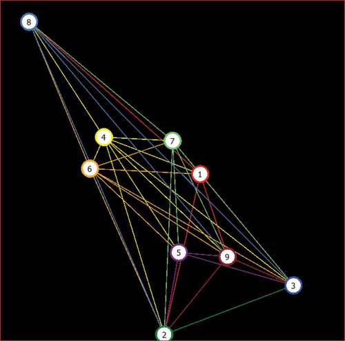
Table 8 presents a clear comparison between alternatives. In Table 8, outranking relations between NTM processes are shown with the help of values of elements from the L, E, and F matrix. {l =1, e = 1, f = 1} shows comparison between two alternatives. While all other combinations show “incomparable” relationships between alternatives. For example, one ranking of alternatives is given by 4-6-7-1-8-5-9-2-3. The sequence for the NTM process can be given as ECM-EDM-WEDM-USM-EBM-CHM-LBM-WJM-AJM in descending order.

Table 8. Outranking relations between NTM processes

Comparison of NTM processes	Cpq	Apq	cpq	apq	l	e	f	Ranking
(1,2)	{2,3,4,5,6,7,9,10}	{1,8}	0.9071	0.223555	1	1	1	1–2
(1,3)	{2,3,4,5,6,7,9,10}	{1,8}	0.9071	0.223395	1	1	1	1–3
(1,4)	{3,5,7}	{1,2,4,6,8,9,10}	0.2113	1	0	0	0	Incomparable
(1,5)	{2,3,5,6,7,10}	{1,4,8,9}	0.5232	0.329152	0	1	0	Incomparable
(1,6)	{2,5,10}	{1,3,4,6,7,8,9}	0.3231	1	0	0	0	Incomparable
(1,7)	{2,5,10}	{1,3,4,6,7,8,9}	0.3231	1	0	0	0	Incomparable
(1,8)	{2,3,6,7,9,10}	{1,4,5,8}	0.7615	0.36575	1	1	1	1–8
(1,9)	{2,3,6,7,8,9,10}	{1,4,5}	0.7761	0.182354	1	1	1	1–9
(2,1)	{1,5,6,8,9,10}	{2,3,4,7}	0.6586	1	0	0	0	Incomparable
(2,3)	{1,3,4,5,6,7,8,9,10}	{2}	0.9389	0.265364	1	1	1	2–3
(2,4)	{5,7,8}	{1,2,3,4,6,9,10}	0.0724	1	0	0	0	Incomparable
(2,5)	{5,6,7,8,10}	{1,2,3,4,9}	0.3232	1	0	0	0	Incomparable
(2,6)	{5,8,10}	{1,2,3,4,6,7,9}	0.2766	1	0	0	0	Incomparable
(2,7)	{5,8,10}	{1,2,3,4,6,7,9}	0.2766	1	0	0	0	Incomparable
(2,8)	{1,2,6,7,8,9,10}	{3,4,5}	0.7009	1	1	0	0	Incomparable
(2,9)	{1,3,6,7,8,9,10}	{2,4,5}	0.7933	1	1	0	0	Incomparable
(3,1)	{1,5,6,8,9,10}	{2,3,4,7}	0.6586	1	0	0	0	Incomparable
(3,2)	{1,2,4,5,6,7,8,9,10}	{3}	0.8465	1	1	0	0	Incomparable
(3,4)	{5,7,8}	{1,2,3,4,6,9,10}	0.0724	1	0	0	0	Incomparable
(3,5)	{5,6,7,8,10}	{1,2,3,4,9}	0.3232	1	0	0	0	Incomparable
(3,6)	{5,8,10}	{1,2,3,4,6,7,9}	0.2766	1	0	0	0	Incomparable
(3,7)	{5,8,10}	{1,2,3,4,6,7,9}	0.2766	1	0	0	0	Incomparable
(3,8)	{1,2,6,7,8,9,10}	{3,4,5}	0.7009	1	1	0	0	Incomparable
(3,9)	{1,3,6,7,8,9,10}	{2,4,5}	0.7933	1	1	0	0	Incomparable
(4,1)	{1,2,4,6,8,9,10}	{3,5,7}	0.7887	0.0943451	1	1	1	4–1
(4,2)	{1,2,3,4,6,8,9,10}	{5,7}	0.9422	0.0467728	1	1	1	4–2
(4,3)	{1,2,3,4,6,8,9,10}	{5,7}	0.9422	0.0467728	1	1	1	4–3
(4,5)	{1,2,3,4,6,7,8,9,10}	{5}	0.9617	0.0234004	1	1	1	4–5
(4,6)	{2,4,8,9,10}	{1,3,5,6,7}	0.6833	0.377492	1	1	1	4–6
(4,7)	{2,4,8,9,10}	{1,3,5,6,7}	0.6833	0.188802	1	1	1	4–7
(4,8)	{1,2,3,4,6,7,8,9,10}	{4,5}	0.9617	0.0701453	1	1	1	4–8
(4,9)	{1,2,3,4,6,7,8,9,10}	{2,5}	0.9617	0.0701453	1	1	1	4–9
(5,1)	{1,4,6,8,9,10}	{2,3,5,7}	0.7276	1	1	0	0	Incomparable
(5,2)	{1,2,3,4,6,8,9,10}	{5,7}	0.9422	0.135947	1	1	1	5–2
(5,3)	{1,2,3,4,6,8,9,10}	{5,7}	0.9422	0.135947	1	1	1	5–3
(5,4)	{1,5,7,8,9}	{2,3,4,6,10}	0.4273	1	0	0	0	Incomparable
(5,6)	{4,8,9,10}	{1,2,3,5,6,7}	0.6222	1	0	0	0	Incomparable
(5,7)	{4,8,9,10}	{1,2,3,5,6,7}	0.6222	1	0	0	0	Incomparable
(5,8)	{1,2,3,6,7,8,9,10}	{4,5}	0.8544	0.570967	1	0	0	Incomparable
(5,9)	{1,3,4,6,7,8,9,10}	{2,5}	0.9006	0.310344	1	1	1	5–9
(6,1)	{1,3,4,5,6,7,8,9,10}	{2}	0.9389	0.114357	1	1	1	6–1
(6,2)	{1,2,3,4,5,6,7,8,9,10}	{}	1	0	1	1	1	6–2
(6,3)	{1,2,3,4,5,6,7,8,9,10}	{}	1	0	1	1	1	6–3
(6,4)	{1,3,5,6,7,8,9}	{2,4,10}	0.6079	1	0	0	0	Incomparable
(6,5)	{1,2,3,4,5,6,7,8,9,10}	{}	1	0	1	1	1	6–5
(6,7)	{1,2,3,4,5,6,7,8,9,10}	{}	1	0	1	1	1	6–7
(6,8)	{1,2,3,6,7,8,9,10}	{4,5}	0.8544	0.114147	1	1	1	6–8
(6,9)	{1,2,3,4,6,7,8,9,10}	{5}	0.9617	0.0309667	1	1	1	6–9
(7,1)	{1,3,4,5,6,7,8,9,10}	{2}	0.9389	0.189302	1	1	1	7–1
(7,2)	{1,2,3,4,5,6,7,8,9,10}	{}	1	0	1	1	1	7–2
(7,3)	{1,2,3,4,5,6,7,8,9,10}	{}	1	0	1	1	1	7–3
(7,4)	{1,3,5,6,7,8,9}	{2,4,10}	0.6079	1	0	0	0	Incomparable
(7,5)	{1,2,3,4,5,6,7,8,9,10}	{}	1	0	1	1	1	7–5
(7,6)	{1,4,5,6,7,8,9,10}	{2,3}	0.7854	1	1	0	0	Incomparable
(7,8)	{1,2,3,6,7,8,9,10}	{4,5}	0.8544	0.152287	1	1	1	7–8
(7,9)	{1,2,3,4,6,7,8,9,10}	{5}	0.9617	0.0412889	1	1	1	7–9
(8,1)	{1,4,5,6,8,9,10}	{2,3,7}	0.7659	1	1	0	0	Incomparable
(8,2)	{1,3,4,5,6,8,9,10}	{2,7}	0.9194	0.0757729	1	1	1	8–2
(8,3)	{1,3,4,5,6,8,9,10}	{2,7}	0.9194	0.0757729	1	1	1	8–3
(8,4)	{5,7,8}	{1,2,3,4,6,9,10}	0.0724	1	0	0	0	Incomparable
(8,5)	{4,5,6,7,8,10}	{1,2,3,9}	0.4305	1	0	0	0	Incomparable
(8,6)	{4,5,8,10}	{1,2,3,6,7,9}	0.3839	1	0	0	0	Incomparable
(8,7)	{4,5,8,10}	{1,2,3,6,7,9}	0.3839	1	0	0	0	Incomparable
(8,9)	{1,3,4,5,6,7,8,9,10}	{2}	0.9389	0.0617143	1	1	1	8–9
(9,1)	{1,4,5,6,8,9,10}	{2,3,7}	0.7659	1	1	0	0	Incomparable
(9,2)	{2,4,5,6,9,10}	{1,3,7,8}	0.7341	0.204125	1	1	1	9–2
(9,3)	{2,4,5,6,9,10}	{1,3,7,8}	0.7341	0.204125	1	1	1	9–3
(9,4)	{5,7}	{1,2,3,4,6,8,9,10}	0.0578	1	0	0	0	Incomparable
(9,5)	{2,4,5,6,7,10}	{1,3,8,9}	0.477	1	0	0	0	Incomparable
(9,6)	{4,5,10}	{1,2,3,6,7,8,9}	0.3693	1	0	0	0	Incomparable
(9,7)	{4,5,10}	{1,2,3,6,7,8,9}	0.3693	1	0	0	0	Incomparable
(9,8)	{2,5,6,7,9,10}	{1,3,4,8}	0.6463	1	0	0	0	Incomparable

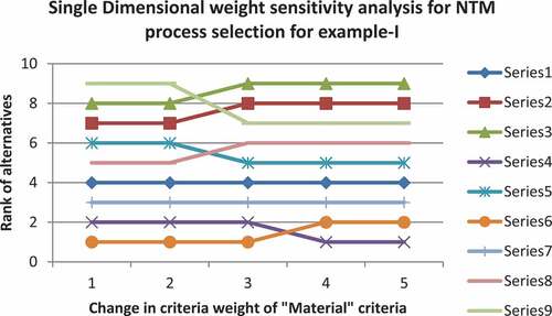
4.1. Single-dimensional weight sensitivity analysis for example-I

SDWSA is done to find the stability range of criteria weight for the criteria having maximum criteria weight value. For example-I “material” criteria is having maximum weight. SDWSA is for the material criteria as shown in the Table 9.

Table 9. Criteria weight variation for single-dimensional weight sensitivity analysis

u1	u2	u3	u4	u5	u6	u7	u8	u9	u10
0.0783	0.0611	0.1535	0.1073	0.0383	0.0271	0.0195	0.0146	0.2766	0.2237
Criteria weight variation with weight additive constraint
0.109	0.0918	0.1842	0.138	0.069	0.0578	0.0502	0.0453	0	0.2544
0.09792	0.08072	0.17312	0.12692	0.05792	0.04672	0.03912	0.03422	0.1	0.24332
0.0868	0.0696	0.162	0.1158	0.0468	0.0356	0.028	0.0231	0.2	0.2322
0.0757	0.0585	0.1509	0.1047	0.0357	0.0245	0.0169	0.012	0.3	0.2296
0.0663	0.0491	0.1415	0.0953	0.0263	0.0151	0.0075	0	0.3846	0.2117

Table 10 presents the rank of alternatives with varying criteria weight. Criteria weight for the material criteria is varied from zero to maximum. The variation comes in the rank of alternatives is observed for the local and global stability range.

Table 10. Alternatives with their ranks for criteria weight variation

Alternative	1	2	3	4	5
o1	4	4	4	4	4
o2	7	7	8	8	8
o3	8	8	9	9	9
o4	2	2	2	1	1
o5	6	6	5	5	5
o6	1	1	1	2	2
o7	3	3	3	3	3
o8	5	5	6	6	6
o9	9	9	7	7	7

Local and global stability ranges for the criteria weight variation are plotted on the graph as shown in Figure 6, where X- axis represents criteria weight variation and Y-axis represents alternative rank variation. Form the Figure 6, the local stability range is between 0 and 0.2 criteria weight, while the global stability range is between 0.3 and 0.3846.

Figure 6. Criteria weight variation for “Material” criteria v/s rank of alternatives.

5. Example-II: selection of NTM process to create efficient machine precision holes on duralumin

N. D. Chakladar & Chakraborty (2008) selected the problem of creating efficient machine precision holes on duralumin and chose nine different NTM processes considering 10 parameters. The decision matrix for the same case is given in Table 11. TSF,PR, and MRR parameters have actual values (quantitative), while the remaining parameters are shown qualitative values with the help of a five-point scale.

Table 11. Decision matrix: performance of various NTM processes to different attributes (N. D. Chakladar & Chakraborty, 2008)

Sr.	Process	Parameters
		u1	u2	u3	u4	u5	u6	u7	u8	u9	u10
1	o1	1.0	10.00	500.0	2	4	2	3	1	4	1
2	o2	2.5	0.22	0.8	1	4	2	2	3	3	1
3	o3	2.5	0.24	0.5	1	4	2	2	3	3	1
4	o4	3.0	100.00	400.0	5	2	3	1	3	5	4
5	o5	3.0	0.40	15.0	3	3	2	1	3	5	4
6	o6	3.5	2.70	800.0	3	4	4	4	3	4	5
7	o7	3.5	2.50	600.0	3	4	4	4	3	4	5
8	o8	2.5	0.20	1.6	4	5	2	1	3	4	1
9	o9	2.0	1.40	0.1	3	5	2	1	1	4	1

Table 12 shows the normalised decision matrix.

Table 12. Normalised decision matrix

Sr.	Process	Parameters
		u1	u2	u3	u4	u5	u6	u7	u8	u9	u10
1	o1	0.1229	0.0994	0.4210	0.2195	0.3345	0.2481	0.4121	0.1240	0.3288	0.1072
2	o2	0.3071	0.0022	0.0007	0.1098	0.3345	0.2481	0.2747	0.3721	0.2466	0.1072
3	o3	0.3071	0.0024	0.0004	0.1098	0.3345	0.2481	0.2747	0.3721	0.2466	0.1072
4	o4	0.3686	0.9943	0.3368	0.5488	0.1672	0.3721	0.1374	0.3721	0.4110	0.4288
5	o5	0.3686	0.0040	0.0126	0.3293	0.2509	0.2481	0.1374	0.3721	0.4110	0.4288
6	o6	0.4300	0.0268	0.6737	0.3293	0.3345	0.4961	0.5494	0.3721	0.3288	0.5361
7	o7	0.4300	0.0249	0.5053	0.3293	0.3345	0.4961	0.5494	0.3721	0.3288	0.5361
8	o8	0.3071	0.0020	0.0013	0.4391	0.4181	0.2481	0.1374	0.3721	0.3288	0.1072
9	o9	0.2457	0.0139	0.0001	0.3293	0.4181	0.2481	0.1374	0.1240	0.3288	0.1072

Pairwise comparison for parameters is given in Table 13, with the help of a nine-point scale. For this example, weights from example-1 are used as the same parameters selected for the NTM process.

Table 13. Pairwise comparison matrix

	u1	u2	u3	u4	u5	u6	u7	u8	u9	u10
u1	1	2	1/3	1/2	3	4	5	6	1/5	1/4
u2	1/2	1	1/3	1/2	2	3	4	5	1/5	1/4
u3	3	3	1	2	5	6	7	8	1/2	1/3
u4	2	2	1/2	1	4	5	6	7	1/4	1/3
u5	1/3	1/2	1/5	1/4	1	2	3	4	1/7	1/6
u6	1/4	1/3	1/6	1/5	1/2	1	2	3	1/8	1/7
u7	1/5	1/4	1/7	1/6	1/3	1/2	1	2	1/9	1/8
u8	1/6	1/5	1/8	1/7	1/4	1/3	1/2	1	1/9	1/9
u9	5	5	2	4	7	8	9	9	1	2
u10	4	4	3	3	6	7	8	9	1/2	1

Equation (2)(2) ${\text{w}}_{\text{\hspace{0.05em}i}}\text{=}\frac{{(\underset{\text{\hspace{0.05em}j=1}}{\overset{}{{{\displaystyle \prod }}^n}}{\text{d}}_{\text{\hspace{0.05em}ij}})}^{\text{\hspace{0.05em}1/n}}}{\underset{\text{\hspace{0.05em}i=1}}{\overset{}{{{\displaystyle \sum }}^n}}{(\underset{\text{\hspace{0.05em}j=1}}{\overset{}{{{\displaystyle \prod }}^n}}{\text{d}}_{\text{\hspace{0.05em}ij}})}^{\text{\hspace{0.05em}1/n}}}\text{i},\text{j=1},\text{2},\text{3}\dots \text{n}$(2) is used to calculate the weights of the criterion. For the example-II, we got values of criterion weights as below:

W_TSF = 0.0783,W_PR = 0.0611, W_MRR = 0.1535, W_C = 0.1073, W_E = 0.0383, W_TF = 0.0271, W_TC = 0.0195, W_S = 0.0146, W_M = 0.2766, W_F = 0.2237.

Equations (6) and (8(8) $\mathrm{CR}=\frac{\mathrm{CI}}{\mathrm{RI}}$(8) ) are used for the evaluation of the maximum Eigen value (λ_max) and consistency ratio (CR). For the pairwise comparison matrix shown in Table 6, λ_max = 10.5749 and CR = 0.0403. It shows consistency, as this value is less than 0.10. It is without any bias.

Equation (10)(10) $\mathrm{Here}{\mathrm{y}}_{\mathrm{ij}}={{\mathrm{b}}_{\mathrm{ij}}}^1+\mathit{\hspace{0.17em}}{{\mathrm{b}}_{\mathrm{ij}}}^2+{{\mathrm{b}}_{\mathrm{ij}}}^3\dots .\dots \mathit{\hspace{0.17em}}.+\mathit{\hspace{0.17em}}{{\mathrm{b}}_{\mathrm{ij}}}^{\mathrm{m}}$(10) and equation (11)(11) $\mathrm{Here}{y}_{\mathit{ij}}={{\mathit{b}}_{\mathit{ij}}}^1+\mathit{\hspace{0.17em}}{{\mathit{b}}_{\mathit{ij}}}^2+{{\mathit{b}}_{\mathit{ij}}}^3\dots .\dots \mathit{\hspace{0.17em}}.+\mathit{\hspace{0.17em}}{{\mathit{b}}_{\mathit{ij}}}^{\mathit{m}}$(11) from the algorithm are implemented on a weighted normalised decision matrix in Table 14. Results are shown in Table 15 as a concordance set and Table 16 as a discordance set.

Table 14. Weighted normalised matrix

Sr.	Parameters
	u1	u2	u3	u4	u5	u6	u7	u8	u9	u10
1	0.0096	0.0061	0.0646	0.0236	0.0128	0.0067	0.0080	0.0018	0.0909	0.0240
2	0.0240	0.0001	0.0001	0.0118	0.0128	0.0067	0.0054	0.0054	0.0682	0.0240
3	0.0240	0.0001	0.0001	0.0118	0.0128	0.0067	0.0054	0.0054	0.0682	0.0240
4	0.0289	0.0607	0.0517	0.0589	0.0064	0.0101	0.0027	0.0054	0.1137	0.0959
5	0.0289	0.0002	0.0019	0.0353	0.0096	0.0067	0.0027	0.0054	0.1137	0.0959
6	0.0337	0.0016	0.1034	0.0353	0.0128	0.0134	0.0107	0.0054	0.0909	0.1199
7	0.0337	0.0015	0.0776	0.0353	0.0128	0.0134	0.0107	0.0054	0.0909	0.1199
8	0.0240	0.0001	0.0002	0.0471	0.0160	0.0067	0.0027	0.0054	0.0909	0.0240
9	0.0192	0.0009	0.0001	0.0353	0.0160	0.0067	0.0027	0.0018	0.0909	0.0240

Table 15. Concordance set

j	1	2	3	4	5	6	7	8	9
C1j	-	{2,3,4,5,6,7,9,10}	{2,3,4,5,6,7,9,10}	{3,5,7}	{2,3,5,6,7}	{2,5,9}	{2,5,9}	{2,3,6,7,9,10}	{2,3,6,7,8,9,10}
C2j	{1,5,6,8,10}	-	{1,3,4,5,6,7,8,9,10}	{5,7,8}	{5,6,7,8}	{5,8}	{5,8}	{1,2,6,7,8,10}	{1,3,6,7,8,10}
C3j	{1,5,6,8,10}	{1,2,4,5,6,7,8,9,10}	-	{5,7,8}	{5,6,7,8}	{5,8}	{5,8}	{1,2,6,7,8,10}	{1,3,6,7,8,10}
C4j	{1,2,4,6,8,9,10}	{1,2,3,4,6,8,9,10}	{1,2,3,4,6,8,9,10}	-	{1,2,3,4,6,7,8,9,10}	{2,4,8,9}	{2,4,8,9}	{1,2,3,4,6,7,8,9,10}	{1,2,3,4,6,7,8,9,10}
C5j	{1,4,6,8,9,10}	{1,2,3,4,6,8,9,10}	{1,2,3,4,6,8,9,10}	{1,5,7,8,9,10}	-	{4,8,9}	{4,8,9}	{1,2,3,6,7,8,9,10}	{1,3,4,6,7,8,9,10}
C6j	{1,3,4,5,6,7,8,9,10}	{1,2,3,4,5,6,7,8,9,10}	{1,2,3,4,5,6,7,8,9,10}	{1,3,5,6,7,8,10}	{1,2,3,4,5,6,7,8,10}	-	{1,2,3,4,5,6,7,8,9,10}	{1,2,3,6,7,8,9,10}	{1,2,3,4,6,7,8,9,10}
C7j	{1,3,4,5,6,7,8,9,10}	{1,2,3,4,5,6,7,8,9,10}	{1,2,3,4,5,6,7,8,9,10}	{1,3,5,6,7,8,10}	{1,2,3,4,5,6,7,8,10}	{1,4,5,6,7,8,9,10}	-	{1,2,3,6,7,8,9,10}	{1,2,3,4,6,7,8,9,10}
C8j	{1,4,5,6,8,9,10}	{1,3,4,5,6,8,9,10}	{1,3,4,5,6,8,9,10}	{5,7,8}	{4,5,6,7,8}	{4,5,8,9}	{4,5,8,9}	-	{1,3,4,5,6,7,8,9,10}
C9j	{1,4,5,6,8,9,10}	{2,4,5,6,9,10}	{2,4,5,6,9,10}	{5,7}	{2,4,5,6,7}	{4,5,9}	{4,5,9}	{2,5,6,7,9,10}	-

Table 16. Discordance set

j	1	2	3	4	5	6	7	8	9
A1j	-	{1,8}	{1,8}	{1,2,4,6,8,9,10}	{1,4,8,9,10}	{1,3,4,6,7,8,10}	{1,3,4,6,7,8,10}	{1,4,5,8}	{1,4,5}
A2j	{2,3,4,7,9}	-	{2}	{1,2,3,4,6,9,10}	{1,2,3,4,9,10}	{1,2,3,4,6,7,9,10}	{1,2,3,4,6,7,9,10}	{3,4,5,9}	{2,4,5,9}
A3j	{2,3,4,7,9}	{3}	-	{1,2,3,4,6,9,10}	{1,2,3,4,9,10}	{1,2,3,4,6,7,9,10}	{1,2,3,4,6,7,9,10}	{3,4,5,9}	{2,4,5,9}
A4j	{3,5,7}	{5,7}	{5,7}	-	{5}	{1,3,5,6,7,10}	{1,3,5,6,7,10}	{5}	{5}
A5j	{2,3,5,7}	{5,7}	{5,7}	{2,3,4,6}	-	{1,2,3,5,6,7,10}	{1,2,3,5,6,7,10}	{4,5}	{2,5}
A6j	{2}	{}	{}	{2,4,9}	{9}	-	{}	{4,5}	{5}
A7j	{2}	{}	{}	{2,4,9}	{9}	{2,3}	-	{4,5}	{5}
A8j	{2,3,7}	{2,7}	{2,7}	{1,2,3,4,6,9,10}	{1,2,3,9,10}	{1,2,3,6,7,10}	{1,2,3,6,7,10}	-	{2}
A9j	{2,3,7}	{1,3,7,8}	{1,3,7,8}	{1,2,3,4,6,8,9,10}	{1,3,8,9,10}	{1,2,3,6,7,8,10}	{1,2,3,6,7,8,10}	{1,3,4,8}	-

Figure 7 represents actual input given in the example-II in the form of a normalized decision matrix.

Figure 7. Actual input is given to the console in the form of a normalised decision matrix and weight obtained from the AHP method for example-II.

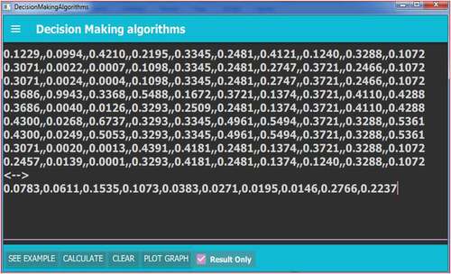
Figure 8 presents summary results for example-II.

Figure 8. Results obtained for the given input data.

The digraph plotted as shown in Figure 9 explains the pictorial presentation of the dominance of one alternative over the other alternative. Appendix-II at the end gives the overall calculations of the mFS ELECTRE-I integrated AHP approach. The decision system developed is useful for the end user that is manager (decision maker) from the manufacturing industry. It is very easy to use console to provide input. Once the decision matrix is ready, it is easy to select the best alternative from the available alternatives. All the decisions obtained with the developed decision system are in line with the decision obtained from the previous work. Furthermore, the decision system helps in improving the performance of the manufacturing process as well as reduces time for decision-making. This type of decision systems can be used in other sectors to take decisions like selection of site for thermal plant, selection of suitable material, selection of best robot, and selection of suitable FMS system.

Figure 9. Directed graph is plotted on the console with C++ code for example-II.

Equation (12) and equation (13) from the algorithm are used to calculate concordance and discordance indices, concordance matrix C, and discordance matrix A results from all such indices.

$\mathit{C}=\left[\begin{array}{ccccccccc}-& 0.9071& 0.9071& 0.2113& 0.5232& 0.3231& 0.3231& 0.7615& 0.7761\\ 0.6586& -& 0.9389& 0.0724& 0.3232& 0.2766& 0.2766& 0.7009& 0.7933\\ 0.6586& 0.8465& -& 0.0724& 0.3232& 0.2766& 0.2766& 0.7009& 0.7933\\ 0.7887& 0.9422& 0.9422& -& 0.9617& 0.6833& 0.6833& 0.9617& 0.9617\\ 0.7276& 0.9244& 0.9422& 0.4273& -& 0.6222& 0.6222& 0.8544& 0.9006\\ 0.9389& 1& 1& 0.6079& 1& -& 1& 0.8544& 0.9617\\ 0.9389& 1& 1& 0.6079& 1& 0.7854& -& 0.8544& 0.9617\\ 0.7659& 0.9194& 0.9194& 0.0724& 0.4305& 0.3839& 0.3839& -& 0.9389\\ 0.7659& 0.7341& 0.7341& 0.0578& 0.477& 0.3693& 0.3693& 0.6463& -\end{array}\right]$

$\mathit{A}=\left[\begin{array}{ccccccccc}-& 0.2235& 0.2233& 1& 0.3291& 1& 1& 0.3657& 0.1823\\ 1& -& 0.2653& 1& 1& 1& 1& 1& 1\\ 1& 1& -& 1& 1& 1& 1& 1& 1\\ 0.0943& 0.0467& 0.0467& -& 0.0234& 0.3774& 0.1888& 0.0701& 0.0701\\ 1& 0.1359& 0.1359& 1& -& 1& 1& 0.5709& 0.3103\\ 0.1143& 0& 0& 1& 0& -& 0& 0.1141& 0.0309\\ 0.1893& 0& 0& 1& 0& 1& -& 0.1522& 0.0412\\ 1& 0.0757& 0.0757& 1& 1& 1& 1& -& 0.0617\\ 1& 0.2041& 0.2041& 1& 1& 1& 1& 1& -\end{array}\right]$

Equation (16) and equation (17)(17) ${\text{e}}_{\text{\hspace{0.05em}pq}}\text{=1},{\text{a}}_{\text{\hspace{0.05em}pq}}\ge \acute{a}\text{ 0},{\text{a}}_{\text{\hspace{0.05em}pq}}\le \acute{a}$(17) are used to evaluate matrices L and E. Finally, matrices L and E emerge as comparison of every element from the matrix with a concordance level of 0.617754 and a discordance level of 0.583391.

$\mathit{L}=\left[\begin{array}{ccccccccc}0& 1& 1& 0& 0& 0& 0& 1& 1\\ 0& 0& 1& 0& 0& 0& 0& 0& 0\\ 0& 1& 0& 0& 0& 0& 0& 0& 0\\ 1& 1& 1& 0& 1& 0& 0& 1& 1\\ 1& 1& 1& 1& 0& 0& 0& 1& 1\\ 1& 1& 1& 0& 1& 0& 1& 1& 1\\ 1& 1& 1& 0& 1& 1& 0& 1& 1\\ 1& 1& 1& 0& 0& 0& 0& 0& 1\\ 1& 1& 1& 0& 0& 0& 0& 1& 0\end{array}\right]$

$\mathit{E}=\left[\begin{array}{ccccccccc}0& 1& 1& 0& 0& 0& 0& 1& 1\\ 0& 0& 1& 0& 0& 0& 0& 0& 0\\ 0& 0& 0& 0& 0& 0& 0& 0& 0\\ 1& 1& 1& 0& 1& 0& 1& 1& 1\\ 0& 1& 1& 0& 0& 0& 0& 1& 1\\ 1& 1& 1& 0& 1& 0& 1& 1& 1\\ 1& 1& 1& 0& 1& 0& 0& 1& 1\\ 0& 1& 1& 0& 0& 0& 0& 0& 1\\ 0& 1& 1& 0& 0& 0& 0& 0& 0\end{array}\right]$

$\mathit{F}=\left[\begin{array}{ccccccccc}0& 1& 1& 0& 0& 0& 0& 1& 1\\ 0& 0& 1& 0& 0& 0& 0& 0& 0\\ 0& 0& 0& 0& 0& 0& 0& 0& 0\\ 1& 1& 1& 0& 1& 0& 0& 1& 1\\ 0& 1& 1& 0& 0& 0& 0& 1& 1\\ 1& 1& 1& 0& 1& 0& 1& 1& 1\\ 1& 1& 1& 0& 1& 0& 0& 1& 1\\ 0& 1& 1& 0& 0& 0& 0& 0& 1\\ 0& 1& 1& 0& 0& 0& 0& 0& 0\end{array}\right]$

Matrix F gives an overlap matrix for matrix L and matrix E. Figure 10 shows a colour-directed graph. Several coloured lines associated with nodes represent a preference for an alternative.

Figure 10. Colour-directed graph, for example-II.

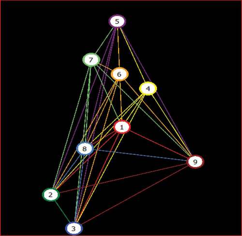
Table 17 provides a straightforward comparison of alternatives. Outranking relationships between NTM processes are shown in Table 17 using values from the L, E, and F matrices. l = 1, e = 1, and f = 1 represent a comparison of two alternatives. While all other combinations show “incomparable” relationships between alternatives, when we calculated number of comparable alternatives the rank order will become 6-4-7-5-1-8-9-2-3. In descending order, the NTM process can be described as EDM-ECM-WEDM-CHM-USM-EBM-LBM-WJM-AJM.

Table 17. Outranking relations between NTM processes

Comparison of NTMP’s	Cpq	Apq	cpq	apq	l	e	f	Ranking
(1,2)	{2,3,4,5,6,7,9,10}	{1,8}	0.9071	0.223555	1	1	1	1–2
(1,3)	{2,3,4,5,6,7,9,10}	{1,8}	0.9071	0.223395	1	1	1	1–3
(1,4)	{3,5,7}	{1,2,4,6,8,9,10}	0.2113	1	0	0	0	Incomparable
(1,5)	{2,3,5,6,7}	{1,4,8,9,10}	0.5232	1	0	0	0	Incomparable
(1,6)	{2,5,9}	{1,3,4,6,7,8,10}	0.3231	1	0	0	0	Incomparable
(1,7)	{2,5,9}	{1,3,4,6,7,8,10}	0.3231	1	0	0	0	Incomparable
(1,8)	{2,3,6,7,9,10}	{1,4,5,8}	0.7615	0.36575	1	1	1	1–8
(1,9)	{2,3,6,7,8,9,10}	{1,4,5}	0.7761	0.182354	1	1	1	1–9
(2,1)	{1,5,6,8,10}	{2,3,4,7,9}	0.382	1	0	0	0	Incomparable
(2,3)	{1,3,4,5,6,7,8,9,10}	{2}	0.9389	0.265364	1	1	1	2–3
(2,4)	{5,7,8}	{1,2,3,4,6,9,10}	0.0724	1	0	0	0	Incomparable
(2,5)	{5,6,7,8}	{1,2,3,4,9,10}	0.0995	1	0	0	0	Incomparable
(2,6)	{5,8}	{1,2,3,4,6,7,9,10}	0.0529	1	0	0	0	Incomparable
(2,7)	{5,8}	{1,2,3,4,6,7,9,10}	0.0529	1	0	0	0	Incomparable
(2,8)	{1,2,6,7,8,10}	{3,4,5,9}	0.4243	1	0	0	0	Incomparable
(2,9)	{1,3,6,7,8,10}	{2,4,5,9}	0.5167	1	0	0	0	Incomparable
(3,1)	{1,5,6,8,10}	{2,3,4,7,9}	0.382	1	1	0	0	Incomparable
(3,2)	{1,2,4,5,6,7,8,9,10}	{3}	0.8465	1	1	0	0	Incomparable
(3,4)	{5,7,8}	{1,2,3,4,6,9,10}	0.0724	1	1	0	0	Incomparable
(3,5)	{5,6,7,8}	{1,2,3,4,9,10}	0.0995	1	1	0	0	Incomparable
(3,6)	{5,8}	{1,2,3,4,6,7,9,10}	0.0529	1	0	0	0	Incomparable
(3,7)	{5,8}	{1,2,3,4,6,7,9,10}	0.0529	1	0	0	0	Incomparable
(3,8)	{1,2,6,7,8,10}	{3,4,5,9}	0.4243	1	1	0	0	Incomparable
(3,9)	{1,3,6,7,8,10}	{2,4,5,9}	0.5167	1	1	0	0	Incomparable
(4,1)	{1,2,4,6,8,9,10}	{3,5,7}	0.7887	0.1796	1	1	1	4–1
(4,2)	{1,2,3,4,6,8,9,10}	{5,7}	0.9422	0.0890	1	1	1	4–2
(4,3)	{1,2,3,4,6,8,9,10}	{5,7}	0.9422	0.0890	1	1	1	4–3
(4,5)	{1,2,3,4,6,7,8,9,10}	{5}	0.9617	0.0529	1	1	1	4–5
(4,6)	{2,4,8,9}	{1,3,5,6,7,10}	0.4596	0.8748	0	0	0	Incomparable
(4,7)	{2,4,8,9}	{1,3,5,6,7,10}	0.4596	0.4366	0	1	0	Incomparable
(4,8)	{1,2,3,4,6,7,8,9,10}	{5}	0.9617	0.1335	1	1	1	4–8
(4,9)	{1,2,3,4,6,7,8,9,10}	{5}	0.9617	0.1335	1	1	1	4–9
(5,1)	{1,4,6,8,9,10}	{2,3,5,7}	0.7276	0.8713	1	0	0	Incomparable
(5,2)	{1,2,3,4,6,8,9,10}	{5,7}	0.9422	0.0445	1	1	1	5–2
(5,3)	{1,2,3,4,6,8,9,10}	{5,7}	0.9422	0.0445	1	1	1	5–3
(5,4)	{1,5,7,8,9,10}	{2,3,4,6}	0.651	1	1	0	0	Incomparable
(5,6)	{4,8,9}	{1,2,3,5,6,7,10}	0.3985	1	0	0	0	Incomparable
(5,7)	{4,8,9}	{1,2,3,5,6,7,10}	0.3985	1	0	0	0	Incomparable
(5,8)	{1,2,3,6,7,8,9,10}	{4,5}	0.8544	0.1637	1	1	1	5–8
(5,9)	{1,3,4,6,7,8,9,10}	{2,5}	0.9006	0.0890	1	1	1	5–9
(6,1)	{1,3,4,5,6,7,8,9,10}	{2}	0.9389	0.0462	1	1	1	6–1
(6,2)	{1,2,3,4,5,6,7,8,9,10}	{}	1	0	1	1	1	6–2
(6,3)	{1,2,3,4,5,6,7,8,9,10}	{}	1	0	1	1	1	6–3
(6,4)	{1,3,5,6,7,8,10}	{2,4,9}	0.555	1	0	0	0	Incomparable
(6,5)	{1,2,3,4,5,6,7,8,10}	{9}	0.7234	0.2240	1	1	1	6–5
(6,7)	{1,2,3,4,5,6,7,8,9,10}	{}	1	0	1	1	1	6–7
(6,8)	{1,2,3,6,7,8,9,10}	{4,5}	0.8544	0.114147	1	1	1	6–8
(6,9)	{1,2,3,4,6,7,8,9,10}	{5}	0.9617	0.0309667	1	1	1	6–9
(7,1)	{1,3,4,5,6,7,8,9,10}	{2}	0.9389	0.0474	1	1	1	7–1
(7,2)	{1,2,3,4,5,6,7,8,9,10}	{}	1	0	1	1	1	7–2
(7,3)	{1,2,3,4,5,6,7,8,9,10}	{}	1	0	1	1	1	7–3
(7,4)	{1,3,5,6,7,8,10}	{2,4,9}	0.555	1	0	0	0	Incomparable
(7,5)	{1,2,3,4,5,6,7,8,10}	{9}	0.7234	0.3006	1	1	1	7–5
(7,6)	{1,4,5,6,7,8,9,10}	{2,3}	0.7854	1	1	0	0	Incomparable
(7,8)	{1,2,3,6,7,8,9,10}	{4,5}	0.8544	0.1227	1	1	1	7–8
(7,9)	{1,2,3,4,6,7,8,9,10}	{5}	0.9617	0.0333	1	1	1	7–9
(8,1)	{1,4,5,6,8,9,10}	{2,3,7}	0.7659	1	1	0	0	Incomparable
(8,2)	{1,3,4,5,6,8,9,10}	{2,7}	0.9194	0.0757729	1	1	1	8–2
(8,3)	{1,3,4,5,6,8,9,10}	{2,7}	0.9194	0.0757729	1	1	1	8–3
(8,4)	{5,7,8}	{1,2,3,4,6,9,10}	0.0724	1	0	0	0	Incomparable
(8,5)	{4,5,6,7,8}	{1,2,3,9,10}	0.2068	1	0	0	0	Incomparable
(8,6)	{4,5,8,9}	{1,2,3,6,7,10}	0.4368	1	0	0	0	Incomparable
(8,7)	{4,5,8,9}	{1,2,3,6,7,10}	0.4368	1	0	0	0	Incomparable
(8,9)	{1,3,4,5,6,7,8,9,10}	{2}	0.9389	0.0617143	1	1	1	8–9
(9,1)	{1,4,5,6,8,9,10}	{2,3,7}	0.7659	1	1	0	0	Incomparable
(9,2)	{2,4,5,6,9,10}	{1,3,7,8}	0.7341	0.204125	1	1	1	9–2
(9,3)	{2,4,5,6,9,10}	{1,3,7,8}	0.7341	0.204125	1	1	1	9–3
(9,4)	{5,7}	{1,2,3,4,6,8,9,10}	0.0578	1	0	0	0	Incomparable
(9,5)	{2,4,5,6,7}	{1,3,8,9,10}	0.2533	1	0	0	0	Incomparable
(9,6)	{4,5,9}	{1,2,3,6,7,8,10}	0.4222	1	0	0	0	Incomparable
(9,7)	{4,5,9}	{1,2,3,6,7,8,10}	0.4222	1	0	0	0	Incomparable
(9,8)	{2,5,6,7,9,10}	{1,3,4,8}	0.6463	1	1	0	0	Incomparable

5.1. Single-dimensional weight sensitivity analysis for example-II

SDWSA is done to find the stability range of criteria weight for the criteria having maximum criteria weight value. For example-I “material” criteria is having maximum weight. SDWSA is for the material criteria as shown in the Table 18.

Table 18. Criteria weight variation for single-dimensional weight sensitivity analysis

u1	u2	u3	u4	u5	u6	u7	u8	u9	u10
0.0783	0.0611	0.1535	0.1073	0.0383	0.0271	0.0195	0.0146	0.2766	0.2237
Criteria weight variation with weight additive constraint
0.109	0.0918	0.1842	0.138	0.069	0.0578	0.0502	0.0453	0	0.2544
0.09792	0.08072	0.17312	0.12692	0.05792	0.04672	0.03912	0.03422	0.1	0.24332
0.0868	0.0696	0.162	0.1158	0.0468	0.0356	0.028	0.0231	0.2	0.2322
0.0757	0.0585	0.1509	0.1047	0.0357	0.0245	0.0169	0.012	0.3	0.2296
0.0663	0.0491	0.1415	0.0953	0.0263	0.0151	0.0075	0	0.3846	0.2117

Table 19 presents the rank of alternatives with varying criteria weight. Criteria weight for the material criteria is varied from zero to maximum. The variation comes in the rank of alternatives is observed for the local and global stability range.

Table 19. Alternatives with their ranks for criteria weight variation

Alternative	1	2	3	4	5
o1	4	4	4	4	4
o2	8	8	8	8	8
o3	9	9	9	9	9
o4	2	2	2	2	1
o5	5	5	5	5	5
o6	1	1	1	1	2
o7	3	3	3	3	3
o8	6	6	6	6	6
o9	7	7	7	7	7

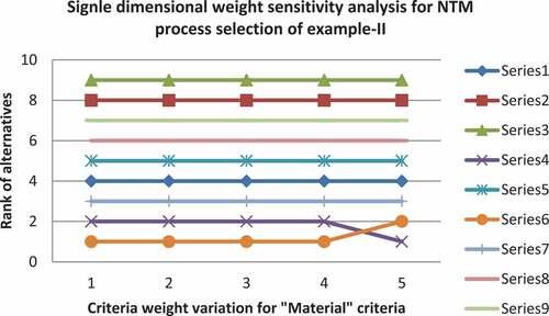
Local and global stability ranges for the criteria weight variation are plotted on the graph as shown in Figure 11, where X- axis presents criteria weight variation and Y-axis presents alternative rank variation. Form Figure 11, the local and global stability ranges are between 0 and 0.3 criteria weight.

Figure 11. Criteria weight variation for “Material” criteria v/s rank of alternatives.

6. Validation of results

Results obtained from example-I and example-II with the mFS ELECTRE-I integrated AHP approach are compared to results obtained in the study by N. D. Chakladar & Chakraborty (2008) (TOPSIS-AHP method), as shown in Table 20. It is observed that the ranks obtained are the same. Karande & Chakraborty (2012) also obtained the results for NTM selection with the PROMETHEE-GAIA method as obtained in Table 20.

Table 20. Validation of results by comparing with the results of N. D. Chakladar & Chakraborty (2008)

	Example-I		Example-II
Ranks	TOPSIS-AHP method (N. D. Chakladar & Chakraborty, 2008)	m-polar ELECTRE-I integrated AHP	TOPSIS-AHP method (N. D. Chakladar & Chakraborty, 2008)	m-polar ELECTRE-I integrated AHP
1	ECM	ECM	EDM	EDM
2	EDM	EDM	ECM	ECM
3	WEDM	WEDM	WEDM	WEDM
4	USM	USM	CHM	CHM
5	EBM	EBM	USM	USM
6	CHM	CHM	EBM	EBM
7	LBM	LBM	LBM	LBM
8	WJM	WJM	WJM	WJM
9	AJM	AJM	AJM	AJM

SDWSA shows that the m-polar fuzzy ELECTRE-I integrated AHP approach gives the local stability range and global stability range for example-I and example-II. For example-I, the local stability range is between 0 and 0.2 and the global stability range is between 0.3 and 0.3846. For example-II, local stability and global stability ranges are between 0 and 0.3. The AHP criteria weight method is suited for the m-polar fuzzy ELECTRE-I as it give stability for criteria weight variation.

7. Conclusions

The rank obtained by the developed decision system implemented in examples I and II is identical to that obtained by the TOPSIS-AHP method, but the advantage of the mFS ELECTRE-I integrated AHP method is that it compares each alternative with other available alternatives with the aid of concordance and discordance indices. As a result, the NTM process can be chosen using the mFS ELECTRE-I integrated AHP algorithm. For instance, it may be inferred from the findings that the ECM is the ideal technique for stainless steel surface revolution. EDM is the optimum method for creating precise holes in duralumin, according to the approved rank, for example-II. Figures 5 and 10 illustrate how the mFS ELECTRE-I integrated AHP algorithm’s implementation offers a clear comparison between two options utilising a colour-directed graph. The decision-making process will take less time, thanks to the soft solution built for the decision system, which also produces the optimum NTM process for the manufacturing process. It gives the decision maker a clearer picture of which NTM method is practical for the specified production demand by contrasting two possibilities with their benefits and drawbacks based on the weights of the criteria. The AHP approach is used with the mFS ELECTRE-I algorithm to assign weights to parameters for the input of mixed (measured and ambiguous) information. We may infer that the mFS ELECTRE-I integrated AHP algorithm can be employed for MCDM and MCGDM based on the examples in this work and the issues solved in the literature. The results of the algorithm are supported by earlier studies (N. D. Chakladar & Chakraborty, 2008; Karande & Chakraborty, 2012), which also demonstrate that the AHP criteria weight variation produced stable rank for NTM processes. It confirms the value of the m-polar fuzzy ELECTRE-I integrated AHP technique even more. Processing the mFS ELECTRE-I for HDWSA is the sensitivity analysis’s restriction. For mFS ELECTRE-I, a procedure for the performance score is not accessible, which restricts HDWSA for the approach. The general algorithm for numerous industrial selection issues is this one. Robot selection, flexible manufacturing system selection, rapid prototyping selection, and other industrial concerns can be taken into account for applications of the mFS ELECTRE-I integrated AHP algorithm. Beyond the nine options covered by the nine trial runs, we can increase the number of options. Most experiments can be computed using the existing soft solution. Even if the highest limits for experiments have not been explored, 25 experiments can be easily evaluated. We can still compare all the possibilities, even though the calculations take more time. The user can assess all possibilities with the help of the current soft solution.

Disclosure statement

No potential conflict of interest was reported by the authors.

Additional information

Funding

The authors received no direct funding for this research.

Notes on contributors

Madan Jagtap

Madan Jagtap is an Assistant Professor in Mechanical Engineering Department in Saraswati College of Engineering, and PhD Research Scholar in Mechanical Engineering Department in the Veermata Jijabai Technological Institute, Matunga, Affiliated to the Mumbai University, Mumbai, India. He earned B.E. in Aeronautical Engineering from Aeronautical Society of India, New Delhi, India. Masters in Manufacturing Systems Engineering from Saraswati College of Engineering Affiliated to Mumbai University, India. He has published journal and conference papers. His research interests include manufacturing, simulation, optimization, reliability and Uncertainty.

Prasad Karande

Prasad Karande is an Associate Professor in Department of Mechanical Engineering at the Veermata Jijabai Technological Institute, Mumbai, India. He earned B.E. in Mechanical Engineering from Shivaji University, India, Masters in Production Engineering with specialization in Manufacturing from Mumbai University, India and PhD in Engineering from Jadavpur University, Kolkata, India. He has published many research papers in leading journal and conferences. Dr. Karande has taught under graduate and post-graduate courses in industrial engineering, operations research, supply chain management etc. His research interests include multi-criteria decision-making, supplier selection, optimization and manufacturing.

Appendix I:

sample calculation for example-I and example-II

0.1229,0.0994,0.4210,0.2195,0.3345,0.2481,0.4121,0.1240,0.2981,0.2041

0.3071,0.0022,0.0007,0.1098,0.3345,0.2481,0.2747,0.3721,0.2981,0.2041

0.3071,0.0024,0.0004,0.1098,0.3345,0.2481,0.2747,0.3721,0.2981,0.2041

0.3686,0.9943,0.3368,0.5488,0.1672,0.3721,0.1374,0.3721,0.3727,0.8165

0.3686,0.0040,0.0126,0.3293,0.2509,0.2481,0.1374,0.3721,0.3727,0.2041

0.4300,0.0268,0.6737,0.3293,0.3345,0.4961,0.5494,0.3721,0.3727,0.2041

0.4300,0.0249,0.5053,0.3293,0.3345,0.4961,0.5494,0.3721,0.3727,0.2041

0.3071,0.0020,0.0013,0.4391,0.4181,0.2481,0.1374,0.3721,0.2981,0.2041

0.2457,0.0139,0.0001,0.3293,0.4181,0.2481,0.1374,0.1240,0.2981,0.2041

<–>

0.0783,0.0611,0.1535,0.1073,0.0383,0.0271,0.0195,0.0146,0.2766,0.2237

===============

Solution:-

Weight multiplied matrix

{{0.00962307},{0.00607334},{0.0646235},{0.0235524},{0.0128114},{0.00672351},{0.00803595},{0.0018104},{0.0824545},{0.0456572}}

{{0.0240459},{0.00013442},{0.00010745},{0.0117815},{0.0128114},{0.00672351},{0.00535665},{0.00543266},{0.0824545},{0.0456572}}

{{0.0240459},{0.00014664},{6.14e-05},{0.0117815},{0.0128114},{0.00672351},{0.00535665},{0.00543266},{0.0824545},{0.0456572}}

{{0.0288614},{0.0607517},{0.0516988},{0.0588862},{0.00640376},{0.0100839},{0.0026793},{0.00543266},{0.103089},{0.182651}}

{{0.0288614},{0.0002444},{0.0019341},{0.0353339},{0.00960947},{0.00672351},{0.0026793},{0.00543266},{0.103089},{0.0456572}}

{{0.033669},{0.00163748},{0.103413},{0.0353339},{0.0128114},{0.0134443},{0.0107133},{0.00543266},{0.103089},{0.0456572}}

{{0.033669},{0.00152139},{0.0775635},{0.0353339},{0.0128114},{0.0134443},{0.0107133},{0.00543266},{0.103089},{0.0456572}}

{{0.0240459},{0.0001222},{0.00019955},{0.0471154},{0.0160132},{0.00672351},{0.0026793},{0.00543266},{0.0824545},{0.0456572}}

{{0.0192383},{0.00084929},{1.535e-05},{0.0353339},{0.0160132},{0.00672351},{0.0026793},{0.0018104},{0.0824545},{0.0456572}}

Vij Matrix

{0.00962307,0.00607334,0.0646235,0.0235524,0.0128114,0.00672351,0.00803595,0.0018104,0.0824545,0.0456572}

{0.0240459,0.00013442,0.00010745,0.0117815,0.0128114,0.00672351,0.00535665,0.00543266,0.0824545,0.0456572}

{0.0240459,0.00014664,6.14e-05,0.0117815,0.0128114,0.00672351,0.00535665,0.00543266,0.0824545,0.0456572}

{0.0288614,0.0607517,0.0516988,0.0588862,0.00640376,0.0100839,0.0026793,0.00543266,0.103089,0.182651}

{0.0288614,0.0002444,0.0019341,0.0353339,0.00960947,0.00672351,0.0026793,0.00543266,0.103089,0.0456572}

{0.033669,0.00163748,0.103413,0.0353339,0.0128114,0.0134443,0.0107133,0.00543266,0.103089,0.0456572}

{0.033669,0.00152139,0.0775635,0.0353339,0.0128114,0.0134443,0.0107133,0.00543266,0.103089,0.0456572}

{0.0240459,0.0001222,0.00019955,0.0471154,0.0160132,0.00672351,0.0026793,0.00543266,0.0824545,0.0456572}

{0.0192383,0.00084929,1.535e-05,0.0353339,0.0160132,0.00672351,0.0026793,0.0018104,0.0824545,0.0456572}

Tabular Concordance Matrix

{{},{2,3,4,5,6,7,9,10},{2,3,4,5,6,7,9,10},{3,5,7},{2,3,5,6,7,10},{2,5,10},{2,5,10},{2,3,6,7,9,10},{2,3,6,7,8,9,10}}

{{1,5,6,8,9,10},{},{1,3,4,5,6,7,8,9,10},{5,7,8},{5,6,7,8,10},{5,8,10},{5,8,10},{1,2,6,7,8,9,10},{1,3,6,7,8,9,10}}

{{1,5,6,8,9,10},{1,2,4,5,6,7,8,9,10},{},{5,7,8},{5,6,7,8,10},{5,8,10},{5,8,10},{1,2,6,7,8,9,10},{1,3,6,7,8,9,10}}

{{1,2,4,6,8,9,10},{1,2,3,4,6,8,9,10},{1,2,3,4,6,8,9,10},{},{1,2,3,4,6,7,8,9,10},{2,4,8,9,10},{2,4,8,9,10},{1,2,3,4,6,7,8,9,10},{1,2,3,4,6,7,8,9,10}}

{{1,4,6,8,9,10},{1,2,3,4,6,8,9,10},{1,2,3,4,6,8,9,10},{1,5,7,8,9},{},{4,8,9,10},{4,8,9,10},{1,2,3,6,7,8,9,10},{1,3,4,6,7,8,9,10}}

{{1,3,4,5,6,7,8,9,10},{1,2,3,4,5,6,7,8,9,10},{1,2,3,4,5,6,7,8,9,10},{1,3,5,6,7,8,9},{1,2,3,4,5,6,7,8,9,10},{},{1,2,3,4,5,6,7,8,9,10},{1,2,3,6,7,8,9,10},{1,2,3,4,6,7,8,9,10}}

{{1,3,4,5,6,7,8,9,10},{1,2,3,4,5,6,7,8,9,10},{1,2,3,4,5,6,7,8,9,10},{1,3,5,6,7,8,9},{1,2,3,4,5,6,7,8,9,10},{1,4,5,6,7,8,9,10},{},{1,2,3,6,7,8,9,10},{1,2,3,4,6,7,8,9,10}}

{{1,4,5,6,8,9,10},{1,3,4,5,6,8,9,10},{1,3,4,5,6,8,9,10},{5,7,8},{4,5,6,7,8,10},{4,5,8,10},{4,5,8,10},{},{1,3,4,5,6,7,8,9,10}}

{{1,4,5,6,8,9,10},{2,4,5,6,9,10},{2,4,5,6,9,10},{5,7},{2,4,5,6,7,10},{4,5,10},{4,5,10},{2,5,6,7,9,10},{}}

F Matrix

{0,0.9071,0.9071,0.2113,0.5232,0.3231,0.3231,0.7615,0.7761}

{0.6586,0,0.9389,0.0724,0.3232,0.2766,0.2766,0.7009,0.7933}

{0.6586,0.8465,0,0.0724,0.3232,0.2766,0.2766,0.7009,0.7933}

{0.7887,0.9422,0.9422,0,0.9617,0.6833,0.6833,0.9617,0.9617}

{0.7276,0.9422,0.9422,0.4273,0,0.6222,0.6222,0.8544,0.9006}

{0.9389,1,1,0.6079,1,0,1,0.8544,0.9617}

{0.9389,1,1,0.6079,1,0.7854,0,0.8544,0.9617}

{0.7659,0.9194,0.9194,0.0724,0.4305,0.3839,0.3839,0,0.9389}

{0.7659,0.7341,0.7341,0.0578,0.477,0.3693,0.3693,0.6463,0}

Concordance level is 0.682832

Tabular Discordance Matrix

{{},{1,8},{1,8},{1,2,4,6,8,9,10},{1,4,8,9},{1,3,4,6,7,8,9},{1,3,4,6,7,8,9},{1,4,5,8},{1,4,5}}

{{2,3,4,7},{},{2},{1,2,3,4,6,9,10},{1,2,3,4,9},{1,2,3,4,6,7,9},{1,2,3,4,6,7,9},{3,4,5},{2,4,5}}

{{2,3,4,7},{3},{},{1,2,3,4,6,9,10},{1,2,3,4,9},{1,2,3,4,6,7,9},{1,2,3,4,6,7,9},{3,4,5},{2,4,5}}

{{3,5,7},{5,7},{5,7},{},{5},{1,3,5,6,7},{1,3,5,6,7},{5},{5}}

{{2,3,5,7},{5,7},{5,7},{2,3,4,6,10},{},{1,2,3,5,6,7},{1,2,3,5,6,7},{4,5},{2,5}}

{{2},{},{},{2,4,10},{},{},{},{4,5},{5}}

{{2},{},{},{2,4,10},{},{2,3},{},{4,5},{5}}

{{2,3,7},{2,7},{2,7},{1,2,3,4,6,9,10},{1,2,3,9},{1,2,3,6,7,9},{1,2,3,6,7,9},{},{2}}

{{2,3,7},{1,3,7,8},{1,3,7,8},{1,2,3,4,6,8,9,10},{1,3,8,9},{1,2,3,6,7,8,9},{1,2,3,6,7,8,9},{1,3,4,8},{}}

G Matrix

{0,0.223555,0.223395,1,0.329152,1,1,0.36575,0.182354}

{1,0,0.265364,1,1,1,1,1,1}

{1,1,0,1,1,1,1,1,1}

{0.0943451,0.0467728,0.0467728,0,0.0234004,0.377492,0.188802,0.0701453,0.0701453}

{1,0.135947,0.135947,1,0,1,1,0.570967,0.310344}

{0.114357,0,0,1,0,0,0,0.114147,0.0309667}

{0.189302,0,0,1,0,1,0,0.152287,0.0412889}

{1,0.0757729,0.0757729,1,1,1,1,0,0.0617143}

{1,0.204125,0.204125,1,1,1,1,1,0}

Discordance level is 0.568396

H Matrix

{0,1,1,0,0,0,0,1,1}

{0,0,1,0,0,0,0,1,1}

{0,1,0,0,0,0,0,1,1}

{1,1,1,0,1,1,1,1,1}

{1,1,1,0,0,0,0,1,1}

{1,1,1,0,1,0,1,1,1}

{1,1,1,0,1,1,0,1,1}

{1,1,1,0,0,0,0,0,1}

{1,1,1,0,0,0,0,0,0}

L Matrix

{0,1,1,0,1,0,0,1,1}

{0,0,1,0,0,0,0,0,0}

{0,0,0,0,0,0,0,0,0}

{1,1,1,0,1,1,1,1,1}

{0,1,1,0,0,0,0,0,1}

{1,1,1,0,1,0,1,1,1}

{1,1,1,0,1,0,0,1,1}

{0,1,1,0,0,0,0,0,1}

{0,1,1,0,0,0,0,0,0}

M Matrix

{0,1,1,0,0,0,0,1,1}

{0,0,1,0,0,0,0,0,0}

{0,0,0,0,0,0,0,0,0}

{1,1,1,0,1,1,1,1,1}

{0,1,1,0,0,0,0,0,1}

{1,1,1,0,1,0,1,1,1}

{1,1,1,0,1,0,0,1,1}

{0,1,1,0,0,0,0,0,1}

{0,1,1,0,0,0,0,0,0}

The best alternative is A4.

Appendix

0.1229,0.0994,0.4210,0.2195,0.3345,0.2481,0.4121,0.1240,0.3288,0.1072

0.3071,0.0022,0.0007,0.1098,0.3345,0.2481,0.2747,0.3721,0.2466,0.1072

0.3071,0.0024,0.0004,0.1098,0.3345,0.2481,0.2747,0.3721,0.2466,0.1072

0.3686,0.9943,0.3368,0.5488,0.1672,0.3721,0.1374,0.3721,0.4110,0.4288

0.3686,0.0040,0.0126,0.3293,0.2509,0.2481,0.1374,0.3721,0.4110,0.4288

0.4300,0.0268,0.6737,0.3293,0.3345,0.4961,0.5494,0.3721,0.3288,0.5361

0.4300,0.0249,0.5053,0.3293,0.3345,0.4961,0.5494,0.3721,0.3288,0.5361

0.3071,0.0020,0.0013,0.4391,0.4181,0.2481,0.1374,0.3721,0.3288,0.1072

0.2457,0.0139,0.0001,0.3293,0.4181,0.2481,0.1374,0.1240,0.3288,0.1072

<–>

0.0783,0.0611,0.1535,0.1073,0.0383,0.0271,0.0195,0.0146,0.2766,0.2237

===============

Solution:-

Weight multiplied matrix

{{0.00962307},{0.00607334},{0.0646235},{0.0235524},{0.0128114},{0.00672351},{0.00803595},{0.0018104},{0.0909461},{0.0239806}}

{{0.0240459},{0.00013442},{0.00010745},{0.0117815},{0.0128114},{0.00672351},{0.00535665},{0.00543266},{0.0682096},{0.0239806}}

{{0.0240459},{0.00014664},{6.14e-05},{0.0117815},{0.0128114},{0.00672351},{0.00535665},{0.00543266},{0.0682096},{0.0239806}}

{{0.0288614},{0.0607517},{0.0516988},{0.0588862},{0.00640376},{0.0100839},{0.0026793},{0.00543266},{0.113683},{0.0959226}}

{{0.0288614},{0.0002444},{0.0019341},{0.0353339},{0.00960947},{0.00672351},{0.0026793},{0.00543266},{0.113683},{0.0959226}}

{{0.033669},{0.00163748},{0.103413},{0.0353339},{0.0128114},{0.0134443},{0.0107133},{0.00543266},{0.0909461},{0.119926}}

{{0.033669},{0.00152139},{0.0775635},{0.0353339},{0.0128114},{0.0134443},{0.0107133},{0.00543266},{0.0909461},{0.119926}}

{{0.0240459},{0.0001222},{0.00019955},{0.0471154},{0.0160132},{0.00672351},{0.0026793},{0.00543266},{0.0909461},{0.0239806}}

{{0.0192383},{0.00084929},{1.535e-05},{0.0353339},{0.0160132},{0.00672351},{0.0026793},{0.0018104},{0.0909461},{0.0239806}}

Vij Matrix

{0.00962307,0.00607334,0.0646235,0.0235524,0.0128114,0.00672351,0.00803595,0.0018104,0.0909461,0.0239806}

{0.0240459,0.00013442,0.00010745,0.0117815,0.0128114,0.00672351,0.00535665,0.00543266,0.0682096,0.0239806}

{0.0240459,0.00014664,6.14e-05,0.0117815,0.0128114,0.00672351,0.00535665,0.00543266,0.0682096,0.0239806}

{0.0288614,0.0607517,0.0516988,0.0588862,0.00640376,0.0100839,0.0026793,0.00543266,0.113683,0.0959226}

{0.0288614,0.0002444,0.0019341,0.0353339,0.00960947,0.00672351,0.0026793,0.00543266,0.113683,0.0959226}

{0.033669,0.00163748,0.103413,0.0353339,0.0128114,0.0134443,0.0107133,0.00543266,0.0909461,0.119926}

{0.033669,0.00152139,0.0775635,0.0353339,0.0128114,0.0134443,0.0107133,0.00543266,0.0909461,0.119926}

{0.0240459,0.0001222,0.00019955,0.0471154,0.0160132,0.00672351,0.0026793,0.00543266,0.0909461,0.0239806}

{0.0192383,0.00084929,1.535e-05,0.0353339,0.0160132,0.00672351,0.0026793,0.0018104,0.0909461,0.0239806}

Tabular Concordance Matrix

{{},{2,3,4,5,6,7,9,10},{2,3,4,5,6,7,9,10},{3,5,7},{2,3,5,6,7},{2,5,9},{2,5,9},{2,3,6,7,9,10},{2,3,6,7,8,9,10}}

{{1,5,6,8,10},{},{1,3,4,5,6,7,8,9,10},{5,7,8},{5,6,7,8},{5,8},{5,8},{1,2,6,7,8,10},{1,3,6,7,8,10}}

{{1,5,6,8,10},{1,2,4,5,6,7,8,9,10},{},{5,7,8},{5,6,7,8},{5,8},{5,8},{1,2,6,7,8,10},{1,3,6,7,8,10}}

{{1,2,4,6,8,9,10},{1,2,3,4,6,8,9,10},{1,2,3,4,6,8,9,10},{},{1,2,3,4,6,7,8,9,10},{2,4,8,9},{2,4,8,9},{1,2,3,4,6,7,8,9,10},{1,2,3,4,6,7,8,9,10}}

{{1,4,6,8,9,10},{1,2,3,4,6,8,9,10},{1,2,3,4,6,8,9,10},{1,5,7,8,9,10},{},{4,8,9},{4,8,9},{1,2,3,6,7,8,9,10},{1,3,4,6,7,8,9,10}}

{{1,3,4,5,6,7,8,9,10},{1,2,3,4,5,6,7,8,9,10},{1,2,3,4,5,6,7,8,9,10},{1,3,5,6,7,8,10},{1,2,3,4,5,6,7,8,10},{},{1,2,3,4,5,6,7,8,9,10},{1,2,3,6,7,8,9,10},{1,2,3,4,6,7,8,9,10}}

{{1,3,4,5,6,7,8,9,10},{1,2,3,4,5,6,7,8,9,10},{1,2,3,4,5,6,7,8,9,10},{1,3,5,6,7,8,10},{1,2,3,4,5,6,7,8,10},{1,4,5,6,7,8,9,10},{},{1,2,3,6,7,8,9,10},{1,2,3,4,6,7,8,9,10}}

{{1,4,5,6,8,9,10},{1,3,4,5,6,8,9,10},{1,3,4,5,6,8,9,10},{5,7,8},{4,5,6,7,8},{4,5,8,9},{4,5,8,9},{},{1,3,4,5,6,7,8,9,10}}

{{1,4,5,6,8,9,10},{2,4,5,6,9,10},{2,4,5,6,9,10},{5,7},{2,4,5,6,7},{4,5,9},{4,5,9},{2,5,6,7,9,10},{}}

F Matrix

{0,0.9071,0.9071,0.2113,0.2995,0.376,0.376,0.7615,0.7761}

{0.382,0,0.9389,0.0724,0.0995,0.0529,0.0529,0.4243,0.5167}

{0.382,0.8465,0,0.0724,0.0995,0.0529,0.0529,0.4243,0.5167}

{0.7887,0.9422,0.9422,0,0.9617,0.4596,0.4596,0.9617,0.9617}

{0.7276,0.9422,0.9422,0.651,0,0.3985,0.3985,0.8544,0.9006}

{0.9389,1,1,0.555,0.7234,0,1,0.8544,0.9617}

{0.9389,1,1,0.555,0.7234,0.7854,0,0.8544,0.9617}

{0.7659,0.9194,0.9194,0.0724,0.2068,0.4368,0.4368,0,0.9389}

{0.7659,0.7341,0.7341,0.0578,0.2533,0.4222,0.4222,0.6463,0}

The concordance level is 0.617754.

Tabular Discordance Matrix

{{},{1,8},{1,8},{1,2,4,6,8,9,10},{1,4,8,9,10},{1,3,4,6,7,8,10},{1,3,4,6,7,8,10},{1,4,5,8},{1,4,5}}

{{2,3,4,7,9},{},{2},{1,2,3,4,6,9,10},{1,2,3,4,9,10},{1,2,3,4,6,7,9,10},{1,2,3,4,6,7,9,10},{3,4,5,9},{2,4,5,9}}

{{2,3,4,7,9},{3},{},{1,2,3,4,6,9,10},{1,2,3,4,9,10},{1,2,3,4,6,7,9,10},{1,2,3,4,6,7,9,10},{3,4,5,9},{2,4,5,9}}

{{3,5,7},{5,7},{5,7},{},{5},{1,3,5,6,7,10},{1,3,5,6,7,10},{5},{5}}

{{2,3,5,7},{5,7},{5,7},{2,3,4,6},{},{1,2,3,5,6,7,10},{1,2,3,5,6,7,10},{4,5},{2,5}}

{{2},{},{},{2,4,9},{9},{},{},{4,5},{5}}

{{2},{},{},{2,4,9},{9},{2,3},{},{4,5},{5}}

{{2,3,7},{2,7},{2,7},{1,2,3,4,6,9,10},{1,2,3,9,10},{1,2,3,6,7,10},{1,2,3,6,7,10},{},{2}}

{{2,3,7},{1,3,7,8},{1,3,7,8},{1,2,3,4,6,8,9,10},{1,3,8,9,10},{1,2,3,6,7,8,10},{1,2,3,6,7,8,10},{1,3,4,8},{}}

G Matrix

{0,0.223555,0.223395,1,1,1,1,0.36575,0.182354}

{1,0,0.265364,1,1,1,1,1,1}

{1,1,0,1,1,1,1,1,1}

{0.179655,0.0890662,0.0890662,0,0.0529805,0.874817,0.436681,0.133573,0.133573}

{0.871389,0.0445065,0.0445065,1,0,1,1,0.163765,0.0890129}

{0.0462334,0,0,1,0.224052,0,0,0.114147,0.0309667}

{0.0474434,0,0,1,0.300631,1,0,0.122795,0.0333721}

{1,0.0757729,0.0757729,1,1,1,1,0,0.0617143}

{1,0.204125,0.204125,1,1,1,1,1,0}

Discordance level is 0.583391.

H Matrix

{0,1,1,0,0,0,0,1,1}

{0,0,1,0,0,0,0,0,0}

{0,1,0,0,0,0,0,0,0}

{1,1,1,0,1,0,0,1,1}

{1,1,1,1,0,0,0,1,1}

{1,1,1,0,1,0,1,1,1}

{1,1,1,0,1,1,0,1,1}

{1,1,1,0,0,0,0,0,1}

{1,1,1,0,0,0,0,1,0}

L Matrix

{0,1,1,0,0,0,0,1,1}

{0,0,1,0,0,0,0,0,0}

{0,0,0,0,0,0,0,0,0}

{1,1,1,0,1,0,1,1,1}

{0,1,1,0,0,0,0,1,1}

{1,1,1,0,1,0,1,1,1}

{1,1,1,0,1,0,0,1,1}

{0,1,1,0,0,0,0,0,1}

{0,1,1,0,0,0,0,0,0}

M Matrix

{0,1,1,0,0,0,0,1,1}

{0,0,1,0,0,0,0,0,0}

{0,0,0,0,0,0,0,0,0}

{1,1,1,0,1,0,0,1,1}

{0,1,1,0,0,0,0,1,1}

{1,1,1,0,1,0,1,1,1}

{1,1,1,0,1,0,0,1,1}

{0,1,1,0,0,0,0,0,1}

{0,1,1,0,0,0,0,0,0}

The best alternative is A6.

References

- Adeel, A., Akram, M., Ahmed, I., & Nazar, K. (2019). Novel m—polar fuzzy linguistic ELECTRE-I method for group decision-making. Symmetry, 11(4), 471. https://doi.org/10.3390/sym11040471
- Adeel, A., Akram, M., & Koam, A. (2019). Multi-criteria decision-making under mHF ELECTRE-I and HmF ELECTRE-I. Energies, 12(9), 1661. https://doi.org/10.3390/en12091661
- Akram, M., Waseem, N., & Liu, P. (2019). Novel approach in decision making with m–polar fuzzy ELECTRE-I. International Journal of Fuzzy Systems, 21(4), 1117–45. https://doi.org/10.1007/s40815-019-00608-y
- Asghari, F., Amidian, A. A., Muhammadi, J., & Rabiee, H. R. (2010). A fuzzy ELECTRE approach for evaluating mobile payment business models. Proceedings - 2010 International Conference on Management of e-Commerce and e-Government, ICMeCG 2010, 351–355. https://doi.org/10.1109/ICMeCG.2010.78
- Aytac, E., Tus, I. A., & Kundakci, N. (2011). Fuzzy ELECTRE I method for evaluating catering firm alternatives. Ege Academic Review, 11(2011), 125–134. http://acikerisim.pau.edu.tr/xmlui/handle/11499/41842
- Boral, S., & Chakraborty, S. (2016). A case-based reasoning approach for non-traditional machining processes selection. Advances in Production Engineering and Management, 11(4), 311–323. https://doi.org/10.14743/apem2016.4.229
- Chakladar, N. D., & Chakraborty, S. (2008). A combined TOPSIS-AHP-method-based approach for non-traditional machining processes selection. Proceedings of the Institution of Mechanical Engineers, Part B: Journal of Engineering Manufacture, 222(12), 1613–1623. https://doi.org/10.1243/09544054JEM1238
- Chakladar, N., Das, R., & Chakraborty, S. (2009). A digraph-based expert system for non-traditional machining processes selection. International Journal of Advanced Manufacturing Technology, 43(3–4), 226–237. https://doi.org/10.1007/s00170-008-1713-0
- Chakrabarti, S., Mitra, S., & Bhattacharyya, B. (2007). Development of an management information system as knowledge base model for machining process characterisation. International Journal of Advanced Manufacturing Technology, 34(11–12), 1088–1097. https://doi.org/10.1007/s00170-006-0673-5
- Chakraborty, S. (2011). Applications of the MOORA method for decision making in manufacturing environment. International Journal of Advanced Manufacturing Technology, 54(9–12), 1155–1166. https://doi.org/10.1007/s00170-010-2972-0
- Chakraborty, S., & Dey, S. (2006). Design of an analytic-hierarchy-process-based expert system for non-traditional machining process selection. International Journal of Advanced Manufacturing Technology, 31(5–6), 490–500. https://doi.org/10.1007/s00170-005-0216-5
- Chakraborty, S., & Dey, S. (2007). QFD-based expert system for non-traditional machining processes selection. Expert Systems with Applications, 32(4), 1208–1217. https://doi.org/10.1016/j.eswa.2006.02.010
- Chatterjee, P., Mondal, S., Boral, S., Banerjee, A., & Chakraborty, S. (2017). A novel hybrid method for non-traditional machining process selection using factor relationship and multi-attribute border approximation method. Facta Universitatis, Series: Mechanical Engineering, 15(3), 439–456. https://doi.org/10.22190/FUME170508024C
- Chen J, Li S, Ma S and Wang X. (2014). m -Polar Fuzzy Sets: An Extension of Bipolar Fuzzy Sets. The Scientific World Journal, 2014 1–8. 10.1155/2014/416530
- Cogun, C. (1993). Computer-aided system for selection of nontraditional machining operations. Computers in Industry, 22(2), 169–179. https://doi.org/10.1016/0166-3615(93)
- Das, S., & Chakraborty, S. (2011). Selection of non-traditional machining processes using analytic network process. Journal of Manufacturing Systems, 30(1), 41–53. https://doi.org/10.1016/j.jmsy.2011.03.003
- Edison Chandrasselan, R., Jehadeesan, R., & Raajenthiren, M. (2008). Web-based knowledge base system for selection of non-traditional machining processes. Malaysian Journal of Computer Science, 21(1), 45–56. https://ejournal.um.edu.my/index.php/MJCS/article/view/6318
- Hatami-Marbini, A., Tavana, M., Moradi, M., & Kangi, F. (2013). A fuzzy group electre method for safety and health assessment in hazardous waste recycling facilities. Safety Science, 51(1), 414–426. https://doi.org/10.1016/j.ssci.2012.08.015
- Jagtap, M., & Karande, P. (2021). Effect of normalization methods on rank performance in single valued mFSELECTRE-I algorithm. Materials Today: Proceedings, Xxxx. https://doi.org/10.1016/j.matpr.2021.10.146
- Jagtap, M., & Karande, P. (2022). Application of M-polar fuzzy set algorithm for non traditional machining process selection. E. Zaramenskikh & A. Fedorova, Eds. Digitalization of society, economics and management. lecture notes in information systems and organisation (Vol. 53, pp. 221–233). Springer. https://doi.org/10.1007/978-3-030-94252-6_16
- Jagtap, M., & Karande, P. (2022). The m-polar fuzzy TOPSIS method for NTM selection. In S. N. Mohanty, P. Chatterjee, & B. T. Hung (Eds.), Fuzzy Computing in Data Science. Wiley. https://doi.org/10.1002/9781394156887.ch15
- Jagtap, M., Karande, P., & Athawale, V. M. (2021). Rank assessment of robots using mFSELECTRE-I algorithm. Proceedings of the International Conference on Industrial Engineering and Operations Management, 246–255. http://ieomsociety.org/sample-reference-paper-9.pdf
- Jagtap, M., Karande, P., & Patil, P. (2022). Modified m-polar fuzzy set ELECTRE-I approach. In S. N. Mohanty, P. Chatterjee, & B. T. Hung (Eds.), Fuzzy computing in data science (pp. 113–145). Wiley. https://doi.org/10.1002/9781394156887.ch7
- Karande, P., & Chakraborty, S. (2012). Application of PROMETHEE-GAIA method for non-traditional machining processes selection. Management Science Letters, 2(6), 2049–2060. https://doi.org/10.5267/j.msl.2012.06.015
- Kaya, T., & Kahraman, C. (2011). An integrated fuzzy AHP-ELECTRE methodology for environmental impact assessment. Expert Systems with Applications, 38(7), 8553–8562. https://doi.org/10.1016/j.eswa.2011.01.057
- Khandekar, A. V., & Chakraborty, S. (2016). Application of fuzzy axiomatic design principles for selection of non-traditional machining processes. International Journal of Advanced Manufacturing Technology, 83(1–4), 529–543. https://doi.org/10.1007/s00170-015-7608-y
- Prasad, K., & Chakraborty, S. (2014). A decision-making model for non-traditional machining processes selection. Decision Science Letters, 3(4), 467–478. https://doi.org/10.5267/j.dsl.2014.7.002
- Prasad, K., & Chakraborty, S. (2018). A decision guidance framework for non-traditional machining processes selection. Ain Shams Engineering Journal, 9(2), 203–214. https://doi.org/10.1016/j.asej.2015.10.013
- Ranjit, R., & Vimalkumar, S. N. (2022). Integrated MOORA-ELECTRE approach for solving multi-criteria decision problem. World Journal of Engineering, 19(4), 510–521. https://doi.org/10.1108/WJE-12-2020-0656
- Recherche, R. O., & Roy, O. B. (1968). Classement et choix en présence de points de vue multiples. Revue Française D’Automatique, D’Informatique Et De recherche opérationnelle. Recherche opérationnelle, tome, 2, 57–75.
- Rouyendegh, B. D., & Erkan, T. E. (2013). An application of the Fuzzy ELECTRE method for academic staff selection. Human Factors and Ergonomics in Manufacturing, 23(2), 107–115.https://doi.org/10.1002/hfm.20301
- Sadhu, A., & Chakraborty, S. (2011). Non-traditional machining processes selection using data envelopment analysis (DEA). Expert Systems with Applications, 38(7), 8770–8781. https://doi.org/10.1016/j.eswa.2011.01.088
- Temuçin, T., Tozan, H., Vayvay, Ö., Harničárová, M., & Valíček, J. (2014). A fuzzy based decision model for nontraditional machining process selection. International Journal of Advanced Manufacturing Technology, 70(9–12), 2275–2282. https://doi.org/10.1007/s00170-013-5474-z
- Yurdakul, M., & Çoǧun, C. (2003). Development of a multi-attribute selection procedure for non-traditional machining processes. Proceedings of the Institution of Mechanical Engineers, Part B: Journal of Engineering Manufacture, 217(7), 993–1009. https://doi.org/10.1243/09544050360686851
- Zadeh, L. (1965). Fuzzy Set. Information and Control, 8, 338–353. https://www-liphy.univ-grenoble-alpes.fr/pagesperso/bahram/biblio/Zadeh_FuzzySetTheory_1965.pdf