Financial performance prediction model based on firms’ internal capability determinants: evidence from listed firms in Thailand during the transition period of going public

Abstract

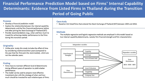
This study attempts to develop a financial performance prediction model, which explores the relationship between the internal capability determinants and the financial performance of public firms both before and after the firms participated in the Stock Exchange of Thailand (SET). The regression and logistic regression methods are employed in this model based on two internal capability determinants, namely firm financial strengths and firm characteristics. The evaluation is based on 111 listed firms that entered the SET between 2003 and 2014, inclusively. Decision makers can make use of the developed model to predict their firms’ financial performance in relative groups (high, medium and low performance groups) during the transition years when they become public. Unlike prior studies, this study includes the effect of time by considering the relative transition years (compared to the year that the firms join the stock market), which are not the calendar years. As a result, the true timing effect on the firm performance before and after going public can be discovered. The empirical evidence shows that the firms have to maintain different levels of determinants during different years of operation to yield a better financial performance. In addition, they can use the results of the prediction to prepare the most effective investment plan with the strategy of when and how much should be invested for each relative type of firms in order to upgrade its financial performance in relative to other firms in the marke

Keywords:

• internal capability determinants
• firm characteristics
• firm financial strengths
• firm performance
• financial prediction model
• logistic regression

1. Introduction

Firms have to deal with several challenges, which can substantially influence their financial performances, during the period of going public. Firms that achieve good performance have the capability to efficiently manage their restricted resources and present competitive advantages over others. To be successful firms, strong determinants that have a significant impact on their performances should be considered. A good understanding of crucial determinants, especially internal capability determinants, which are controllable by the firms, can lead to a superior performance.

Many past studies (e.g., Bătae et al., 2021; Ghosh, 2008; Sinthupundaja & Chiadamrong, 2017; Teeratansirikool et al., 2013; Wattanawarangkoon et al., 2022) have investigated the relationship between determinants of internal capabilities and firm performance. According to these studies, the firms would know the determinants they should emphasize, but they do not know what exactly will happen after focusing on these determinants. On the other hand, other studies (e.g., Bose & Pal, 2006; He et al., 2022; Zhang et al., 1999) have focused on developing firm performance prediction models. These studies can only utilize the prediction models to forecast the firm status, but these studies ignore the effect of significant determinants. Evaluating the firms’ performance in order to know both their financial health and how to improve their performances would be a powerful tool to help decision makers or managers make good business decisions. Furthermore, most of the past studies, which investigated such relationships, have done the analysis based on the calendar year (not the relative transition year when a firm becomes public) so that the characteristics and actual status of the firms during the transition period cannot be depicted appropriately.

Therefore, the objective of this study is to develop a firm financial performance prediction model and explore the relationship between the internal capability determinants and the financial performance of public firms both before and after the firms participated in the Stock Exchange of Thailand (SET) based on the relative transition years. The regression and logistic regression methods are employed in order to construct the prediction model for each specific relative year in the transition period from one year before through four years after the firms enter the stock market. The analyses are performed based on 111 firms listed in the SET (collection period of the data from 2002 to 2018). The main contributions of this study are summarized as follows:

• Developing the financial performance prediction model based on the internal capability determinants before and after the firms become public

• Including the effect of time by considering the relative transition years (compared to the year that the firms join the stock market), which are not the calendar years

• Exploring the relationship between interested factors (derived from the internal capability determinants) and financial performance as well as identifying how the firms can improve their financial performance through improving their internal capability determinants

• Providing the recommendations (e.g., when and how much to invest) for achieving a better performance to the firms during this transition period

The study is organized as follows. Section 2 presents the related literature showing the review of related literature and research gap. Section 3 addresses the research design explaining the data, samples, measures of variables and conceptual framework. Section 4 provides the results and discussion. Section 5 delivers the managerial implications through another application of the prediction model. Section 6 then illustrates the financial performance prediction tool and the last section states the conclusions, limitations, and recommendations for further research.

2. Literature review

Performance predictions can play an important role in business and financial decisions. With performance prediction models, significant determinants can be determined, and good decisions can be made leading firms to achieve a good performance. The firm financial performance predictions and relationships between firm performance and determinants have been studied by many researchers. Depending on the aims of the studies, different variables of determinants and different techniques have been used. Abor (2005), Altaf and Shah (2018) and Ahmed and Afza (2019) developed the performance prediction models by applying multiple regression, a statistical technique, to explore the impact of capital structure on firm performance and profitability. With the same technique, Babalola (2013) investigated the relationship between firm size and the profitability of listed manufacturing firms in the Nigerian Stock Exchange. Ghafoorifard et al. (2014) employed the linear regression method to develop the financial prediction models for listed firms in the Tehran Stock Exchange using firm size and age as predictors. Dagestani and Qing (2022) highlighted the use of Environmental Information Disclosure (EID) practices as a means to improve a firm’s reputation and stakeholder support in resulting in a positive impact on firm financial performance in China. On the other hand, Lam (2004) applied one of the machine learning techniques, namely neural networks, to construct the financial performance prediction models including 16 financial statements and 11 macroeconomic variables for S&P companies. Ravi et al. (2008) also presented bank performance prediction models by employing a number of machine learning techniques, including a Probabilistic Neural Network (PNN) and a Radial Basis Function Neural Network (RBFNN), Support Vector Machine (SVM), and Classification and Regression Trees (CART).

Regarding the internal capabilities, the scope of this study is focused on two internal determinants, firm financial strengths and firm characteristics. Both the capability and the status of firms can be explained through these two determinants. The firms can obtain a good performance when the levels of these determinants are properly controlled (Abor, 2005; Babalola, 2013; Banafa et al., 2015; Bongoye et al., 2016; Fazlzadeh et al., 2011; Ghafoorifard et al., 2014; Ghosh, 2008; Harvey et al., 2001; Nasrallah & El Khoury, 2022; Wan Yusoff & Alhaji, 2012).

The financial strengths reveal firms’ financial power. A firm with more financial power tends to have a better financial position, and a better financial position can lead the firm to achieve a better performance. Furthermore, the financial strengths can indicate the capability of firms to control the amount of cash, expense and working capital. Liquidity, leverage and the cost of goods sold can be employed as indicators to assess the financial strengths.

Liquidity can have an impact on a firm performance since it represents the ability to efficiently make use of working capital and quickly convert a firm’s assets to cash. Kim et al. (1998) stated that handling unexpected situation and uncertainty are more preferable to firms that have higher liquidity, and these firms usually achieve a good performance. On the other hand, Hvide and Møen (2007) claimed that instead of a high level of liquidity, a moderate level can better lead to a superior performance. As a result, the impact of liquidity on the firm performance is still ambiguous.

Leverage is often considered as one of the critical factors contributing to the performance of the firms. A positive association between leverage and performance was discovered (Muritala, 2012). Higher leverage can decrease the agency cost and inefficiency resulting in a better performance. However, too high leverage brings greater risk, which can harm the firm performance. Aburisheh et al. (2022) reported that financial leverage has a beneficial impact on earnings management in the industrial firms listed in the Amman Stock Exchange as the higher financial leverage of the firms, the greater the inclination to commit accruals.

Cost of goods sold includes all product or service relevant costs. If the cost is lowered, firms can have a higher competitive advantage over others. Pasiouras and Kosmidou (2007) conducted an experiment to study the effect of the cost to income ratio on bank performance. The negative association between the cost ratio and performance was found indicating that to obtain high performance, cost must be low. The impact of the cost of sales to the sales ratio on the performance of healthcare firms was also studied by Park and Guahk (2017). The results showed that lowering the cost of sales allows firms to spend more on their research and development projects so that corporate value and firm profitability are then increased.

Firm characteristics present the ability of firms to remain competitive and explain the physical condition of firms. The firm characteristics are generally measured by asset utilization, tangibility of assets and firm size.

Asset utilization indicates the efficiency of firms to utilize their assets in order to generate revenue or sales (Ablanedo-Rosas et al., 2010). Seema and Surendra (2011) discovered that asset utilization significantly affects the firm financial performance in the way that higher asset utilization results in a better performance.

Asset tangibility is also one of the determinants that can have an impact on a firm performance. Jensen and Meckling (1976) defined it as the proportion of fixed assets in total assets. Tangibility is reported to have a positive relationship with firm performance (Ahmed et al., 2010). Higher amount of revenue can be generated thanks to a higher amount of fixed assets. In contrast, an excess amount of fixed assets can harm the firm performance if the fixed assets are not utilized efficiently.

Company size or firm size represents the total asset owned by the firm. The accurate association between company size and firm performance is still not agreed upon. Flamini et al. (2009) and Almajali et al. (2012) stated that a better performance is favorable for larger firms since they will have more competitive power to survive in a highly competitive market. Moreover, larger firms can better exploit economies of scale to reduce cost and increase profit. On the other hand, Majumdar (1997) insisted that large firms may achieve inferior performance due to an inefficient use of their assets, while Aburisheh et al. (2022) demonstrated that company size has no or little impact on earnings management for industrial firms listed on Amman Stock Exchange.

Firm performance indicates the capability of a firm to acquire and utilize its resources in order to develop a competitive advantage over others. Several measures can be used to represent the firm performance such as Return on Assets (ROA), Return on Equity (ROE), Return on Sales (ROS), Return on Investment (ROI) and Tobin’s Q. Different researchers may employ different measures to address different views of performance. Ghosh (2008) used ROA to examine the association between factors of capital structure and firm performance. On the other hand, Liargovas and Skandalis (2010) explored the effects of internal determinants toward three measures of performance, namely ROA, ROE and ROS.

The importance (consideration) of timing effect has been determined differently among past studies. Harvey et al. (2001), Ghosh (2008), Fazlzadeh et al. (2011) and Ghafoorifard et al. (2014) simultaneously analyzed all data from different years during the specified period. According to these analyses, the relationship between firm performance and determinants over the period of interest could be investigated, but the relationship in each year is still undetermined. On the other hand, Wan Yusoff and Alhaji (2012) separately analyzed the data in each calendar year during the specified period. The effect of time is considered in this case so that the relationship between determinants and firm performance in each year could be discovered. In this study, the effect of time is taken into consideration. Nevertheless, instead of doing the analyses based on the calendar years, the analysis is determined the relative transition period years during the firm joined the stock market. As a result, the true timing effect on the firm performance before and after going public can be discovered. Table 1 summarizes the literature related to determinants, firm performance, timing effect, and analysis techniques. The research gap is also highlighted in this table.

Table 1. A literature summary and research gap

Study	Determinants							Firm Performance				Timing Effect			Analysis Techniques
	Liquidity	Leverage	Cost of goods sold	Company size	Asset Utilization	Tangibility	Others^1	ROA	ROE	ROS	Others^2	Not Include	Calendar Year	Relative Transition Year
Majumdar (1997)	✓	✓		✓		✓	✓				✓		✓		Multiple Regression
Opler et al. (1999)					✓		✓					✓			T-Test and Multiple Regression
Harvey et al. (2001)		✓		✓		✓	✓				✓	✓			Regression
Lam (2004)	✓				✓		✓		✓				✓		Neural Networks
Pasiouras and Kosmidou (2007)	✓			✓			✓	✓				✓			Multiple Regression
Ghosh (2008)		✓		✓		✓		✓				✓			Multiple Regression
Ravi et al. (2008)	✓	✓					✓				✓		✓		Neural Network, Support Vector Machine
Liargovas and Skandalis (2010)	✓	✓		✓		✓	✓	✓	✓	✓		✓			Multiple Regression
Fazlzadeh et al. (2011)	✓	✓		✓			✓	✓			✓	✓			F-Test, T-Test, and Multiple Regression
Seema and Surendra (2011)	✓	✓					✓	✓	✓		✓		✓		Paired T-test and Independent T-Test
Almajali et al. (2012)	✓	✓		✓			✓	✓				✓			T-test and Multiple Regression
Muritala (2012)		✓		✓	✓	✓	✓	✓	✓			✓			Multiple Regression
Olson et al. (2012)			✓	✓	✓		✓				✓	✓			Logistic Regression, Decision Tree, Neural Network and Support Vector Machines
Wan Yusoff and Alhaji (2012)							✓		✓		✓		✓		Spearman’s Correlation Matrix
Babalola (2013)	✓	✓		✓			✓	✓				✓			Multiple Regression
Ghafoorifard et al. (2014)				✓							✓	✓			Linear Regression
Abor (2005)		✓		✓					✓			✓			Multiple Regression
Banafa et al. (2015)		✓						✓			✓	✓			T-Test
Bongoye et al. (2016)	✓			✓		✓	✓	✓				✓			T-Test
Park and Guahk (2017)		✓			✓		✓	✓	✓	✓	✓	✓			Multiple Regression
Altaf and Shah (2018)	✓	✓		✓			✓	✓			✓	✓			Multiple Regression
Ahmed and Afza (2019)	✓	✓		✓		✓	✓	✓	✓		✓	✓			Multiple Regression
Le Thi Kim et al. (2021)	✓	✓		✓	✓		✓		✓	✓		✓			Linear Regression and Blinder–Oaxaca decomposition analysis
Nasrallah and El Khoury (2022)				✓			✓	✓			✓	✓			Multiple Regression
This Study	✓	✓	✓	✓	✓	✓		✓	✓	✓				✓	Logistic Regression and Multiple Regression

Remarks: (1) Other determinants include Competitive intensity, Risk, Growth opportunity, Company age, Investment and management efficiency, etc.

(2) Other financial performances include Sales, Net profit, Tobin’s Q, Return on Investment, Earnings before Interest and Taxes and etc.

3. Research design

3.1. Data and sample

Firms listed in SET are investigated in this study. The firms are divided into eight industries, namely Technology, Property & Construction, Financials, Agro & Food Industry, Resources, Industrials, Services and Consumer Products. Firms in Financials and Services industries are excluded due to their different financial structures as they provide services instead of products. The financial data of each firm for five years (from one year before through four years after the firm became listed in the SET) are collected. As illustrated in Figure 1, if firm A joined the SET in 2008, this firm’s financial data in 2007 and from 2009 to 2012 will be collected. Similarly, if firm B joined the SET in 2010, this firm’s financial data in 2009 and from 2011 to 2014 will be collected. Considering each data set, the data of each firm can be retrieved from a different calendar year as the data set for the second year after the firms became listed is the data in 2010 for firm A but it is the data set in 2012 for firm B.

Figure 1. Timeline Overview.

Since the available financial data are limited, this study includes only the firms that participated in SET between 2003 and 2014. As a result, the data collection period is from 2002 to 2018. During this period, 123 interested firms joined the SET (not including financial and service firms). However, as a consequence of newly opening, going bankrupt, ceasing or merging with other firms, the financial data of some firms are absent, and these firms are then excluded from the analysis. As a result, only 111 firms or 90% of the listed firms remain in the analysis, as presented in Tables 2 and 3.

Table 2. Number of firms as classified by industry groups

Industry group	No. of firms
Agro & Food Industry	12
Consumer Products	5
Industrials	16
Property & Construction	43
Resources	14
Technology	21
Total	111

Table 3. Number of new listed firms in each year

Year	No. of firms
2014	12
2013	6
2012	3
2011	2
2010	3
2009	4
2008	7
2007	5
2006	8
2005	24
2004	23
2003	14
Total	111

To obtain the data required for this study, the income statement and the balance sheet must be explored. The balance sheet presents the assets, liabilities and shareholder’s equity of the firm. The income statement reports all revenues and costs incurred by the operation of the firm. These two financial statements can be found in the annual report of each firm and can be accessed through the websites of the SET, the Securities and Exchange Commission (SEC), and the firms. The determinants and performance for the analysis will be found using the collected data.

3.2. Measure of variables

3.2.1. Dependent variable

The dependent variable employed in this study is firm financial performance, which can be indicated by the combination of ROA, ROE and ROS (Sinthupundaja & Chiadamrong, 2017; Waddock & Graves, 1997). With these three measures, all aspects of financial performance can be covered. ROA is measured by the ratio of net income to total assets. It can provide the information about how efficiently a firm is operated (Petersen & Schoeman, 2008). ROE is calculated by the net income divided by total shareholders’ equity. It reveals the shareholders’ return on investment (Kabajeh et al., 2012). ROS is measured by the ratio of net income to total sales. It analyzes the percentage of sales that results in net income (Eva & Roman, 2018). The combination of the three measures can provide the overview of the firms’ financial performance as it can point out the internal efficiency and internal capability of the firms to generate the profit (Cochran & Wood, 1984; Orlitzky et al., 2003). Table 4 presents the dependent variable and their definition used in the analyses.

Table 4. Definition of dependent variable

Dependent Variable		Definition
Firm financial performance	Combination of ROA, ROE, ROS	ROA + ROE + ROS
	ROA	Net income/Total assets
	ROE	Net income/Total shareholders’ equity
	ROS	Net income/Total sales

3.3. Independent variables

There are six independent variables including factors of firm financial strengths and firm characteristics. The firm financial strengths include three variables, which are liquidity, leverage and Cost of Goods Sold (COGS). According to Mehari and Aemiro (2013), the current ratio is used to evaluate liquidity as it can measure the firm’s capability to handle its short-term obligations. It is a proportion of current assets to current liabilities. Leverage reveals the proportion of obligations in the capital structure and is measured by the debt ratio (Rajan & Zingales, 1995). It is the ratio of total liabilities to total assets. COGS is defined by the ratio of cost of goods sold to total sales. According to Krisnanto (2016), COGS refers to all cost related to products or services. The COGS ratio reflects how efficiently a firm manages its cost in relation to its sales.

The firm characteristics include another three variables, which are asset utilization, tangibility and company size. As suggested by Ellis (1998), asset utilization demonstrates the ability of a firm to utilize its assets. It is measured by the asset turnover ratio or the ratio of net sales to total assets. Jensen and Meckling (1976) used the proportion of fixed assets to total assets to represent tangibility. Company size can be assessed by several measurements. One of them is a natural logarithm of total assets (Hensher et al., 2007). It illustrates the size of a firm as the amount of total assets. These six independent variables can capture all business operations within the firms as any business transactions within the firms can be detected through these six variables. The independent variables and their definitions used in the analyses are presented in Table 5.

Table 5. Definitions of independent variables

Independent Variable		Definition
Firm financial strengths	Liquidity	Total current assets/Total current liability	X1
	Leverage	Total liabilities/Total assets	X2
	COGS	Cost of goods sold/Total sales	X3
Firm characteristics	Asset utilization	Total sales/Total assets	X4
	Tangibility	Total fixed assets/Total assets	X5
	Company size	ln(Total assets)	X6

3.4. Analysis techniques

In this study, financial performance prediction models are developed using two statistical techniques, including multiple regression and logistic regression. Both techniques are employed and compared to identify their benefits and drawbacks. The superior technique will be selected for further analysis. The two techniques are explained as follows:

3.4.1. Multiple regression

Multiple regression is a popular analytic method commonly used in educational and behavioural sciences (Kelley et al., 2013). Many researchers adopt this method in the field of business and finance since it can provide a way to quantitatively model an outcome via the use of regressors. It attempts to model the variation of a dependent variable or an outcome as a function of independent variables or regressors. A multiple regression model is presented in Equation 1.(1) $\mathit{Y}={\beta }_0+{\beta }_1{X}_1+{\beta }_2{X}_2+{\beta }_3{X}_3+\dots +X_n{\beta }_n+{\beta }_{12}{X}_1{X}_2+{\beta }_{13}{X}_1{X}_3+\dots +{\beta }_{\mathit{n}-1,\mathit{n}}{X}_{\mathit{n}-1}{X}_n$(1)

(1) $\mathit{Y}={\beta }_0+{\beta }_1{X}_1+{\beta }_2{X}_2+{\beta }_3{X}_3+\dots +X_n{\beta }_n+{\beta }_{12}{X}_1{X}_2+{\beta }_{13}{X}_1{X}_3+\dots +{\beta }_{\mathit{n}-1,\mathit{n}}{X}_{\mathit{n}-1}{X}_n$(1)

where: $\mathit{Y}$ = the dependent variable

${\beta }_0$ = the intercept

${\beta }_1$ to ${\beta }_n$ = the estimated coefficient of $X_1$ to $X_n$

${\beta }_{12}$ to ${\beta }_{\mathit{n}-1,\mathit{n}}$ = the estimated coefficient of $X_{12}$ to $X_{\mathit{n}-1,\mathit{n}}$

$X_1$ to $X_n$ = the independent variables

$\mathit{n}$ = the total number of independent variables

3.4.2. Logistic regression

Logistic regression or logit model is another popular analytic technique applied in business and financial research (Youn & Gu, 2010). It is a method for estimating the probability of a desired event or the group membership of independent variables using the logistic transformation of dependent variables (Öğüt et al., 2012). This study employs two logistic models, including binary logistic regression for two possible outcome and ordinal logistic regression for three-or-more possible outcome. A logistic regression model is presented in Equation 2.(2) $\mathit{Log}\left(\frac{p}{1-\mathit{p}}\right)={\beta }_0+{\beta }_1{X}_1+{\beta }_2{X}_2+{\beta }_3{X}_3+\dots +X_n{\beta }_n+{\beta }_{12}{X}_1{X}_2+\dots +{\beta }_{\mathit{n}-1,\mathit{n}}{X}_{\mathit{n}-1}{X}_n$(2)

(2) $\mathit{Log}\left(\frac{p}{1-\mathit{p}}\right)={\beta }_0+{\beta }_1{X}_1+{\beta }_2{X}_2+{\beta }_3{X}_3+\dots +X_n{\beta }_n+{\beta }_{12}{X}_1{X}_2+\dots +{\beta }_{\mathit{n}-1,\mathit{n}}{X}_{\mathit{n}-1}{X}_n$(2)

where: $\mathit{p}$ = the probability that the desired event will occur

${\beta }_0$ = the intercept

${\beta }_1$ to ${\beta }_n$ = the estimated coefficient of $X_1$ to $X_n$

${\beta }_{12}$ to ${\beta }_{\mathit{n}-1,\mathit{n}}$ = the estimated coefficient of $X_{12}$ to $X_{\mathit{n}-1,\mathit{n}}$

$X_1$ to $X_n$ = the independent variables

$\mathit{n}$ = the total number of independent variables

According to the binary logistic regression model, the probability of the desired event that will occur ($\mathit{p}$) can be calculated as follows:

(3) $\mathit{p}=\frac{e^{{\beta }_0+{\beta }_1{X}_1+{\beta }_2{X}_2+{\beta }_3{X}_3+\dots +X_n{\beta }_n+{\beta }_{12}{X}_1{X}_2+\dots +{\beta }_{\mathit{n}-1,\mathit{n}}{X}_{\mathit{n}-1}{X}_n}}{1+e^{{\beta }_0+{\beta }_1{X}_1+{\beta }_2{X}_2+{\beta }_3{X}_3+\dots +X_n{\beta }_n+{\beta }_{12}{X}_1{X}_2+\dots +{\beta }_{\mathit{n}-1,\mathit{n}}{X}_{\mathit{n}-1}{X}_n}}$(3)

3.5. Conceptual framework

Both statistical techniques, multiple regression and logistic regression are employed to develop prediction models and analyze the relationship between the six independent variables and the firm financial performance. The conceptual framework is presented in Figure 2. The financial data in each dataset (in each year relatively to the year that the firm participated in SET) will be analyzed separately. Therefore, five models will be obtained from each technique.

Figure 2. Conceptual framework.

4. Results and discussion

4.1. Correlation test

Correlation is tested to check whether there is an association among the independent variables or not. As suggested by Akoglu (2018), a correlation coefficient of 0.7 or higher will indicate a strong relationship between variables. If the correlation between any two independent variables is too high, one of them should be removed from the model in order to prevent the problem of multicollinearity that can lead to the misinterpretation of results. The correlation test is performed separately for each dataset (in each year relatively to the year that the firm participated in SET). For example, Table 6 presents the Pearson’s correlation coefficients between any two independent variables for the dataset of one year before the firm participating in SET. The results reveal a maximum correlation coefficient of 0.357 between asset utilization and cost of goods sold. No value of correlation between any two variables is higher than 0.7 in all tested relative years. It is indicated that the regression models containing the aforementioned six independent variables in all relative years are valid and do not have the problem of multicollinearity.

Table 6. Pearson’s correlation coefficient of the case with one year before becoming public firms

Condition	Liquidity	Leverage	Cost of goods sold ratio	Asset utilization	Tangibility	Company size
Liquidity	1
Leverage	−0.201	1
Cost of goods sold	−0.040	0.207	1
Asset utilization	−0.201	−0.075	0.357	1
Tangibility	−0.232	−0.141	−0.245	−0.101	1
Company size	−0.048	−0.095	0.046	−0.043	0.352	1

4.2. Performance prediction models

4.2.1. Multiple regression

For the multiple regression analysis, Minitab 19 is used to analyze financial data using a combination of ROA, ROE and ROS as a dependent variable and six aforementioned variables as independent variables. Prior to the analysis, all variables are standardized by subtracting the mean and then dividing by the standard deviation in order to get rid of bias due to the differences in the scales of the variables. Interactions among variables are allowed up to the second degree. Applying the backward elimination method, the terms that have a p-value exceeding 0.10 will be eliminated from the model. The final model will be obtained when there are only significant terms (p-value ≤0.10) in the model. It should be noted that if the interaction of any two factors is significant, these two factors will remain in the model, whether they are significant or not. Equations 4(4) $\mathit{Y}=-2.21-0.1220X_1-0.059X_2-0.674X_3+0.648X_4+5.70X_5+0.1353X_6+0.1416X_1{X}_2+0.1381X_1{X}_4-0.784X_3{X}_4-0.2503X_5{X}_6$(4) to 8(8) $\mathit{Y}=-6.12+0.229X_1+1.1538X_2+6.72X_3+1.005X_4-0.299X_5+0.2628X_6+0.0274X_1{X}_2+0.1619X_1{X}_5-0.01403X_1{X}_6-1.2517X_2{X}_3-1.025X_3{X}_4-0.280X_3{X}_6$(8) present the final regression model in each year.

Multiple regression model for one year before becoming public firms

(4) $\mathit{Y}=-2.21-0.1220X_1-0.059X_2-0.674X_3+0.648X_4+5.70X_5+0.1353X_6+0.1416X_1{X}_2+0.1381X_1{X}_4-0.784X_3{X}_4-0.2503X_5{X}_6$(4)

The multiple regression model for 1^st year after becoming public firms

(5) $\mathit{Y}=-0.366+0.0072X_1+0.1042X_2-0.175X_3+0.623X_4-0.082X_5+0.0258X_6+0.1143X_1{X}_5-0.639X_3{X}_4$(5)

The multiple regression model for 2^nd year after becoming public firms

(6) $\mathit{Y}=-2.835-0.2291X_1-0.655X_2+1.962X_3+2.055X_4+0.1279X_5+1.962X_6+0.1340X_1{X}_2+0.3097X_1{X}_4+1.322X_2{X}_5-4.802X_3{X}_5+1.366X_4{X}_5-0.1414X_4{X}_6$(6)

The multiple regression model for 3^rd year after becoming public firms

(7) $\mathit{Y}=-2.351-0.362X_1+1.721X_2+2.499X_3+1.466X_4+2.233X_5+0.0121X_6+0.01837X_1{X}_6-1.949X_2{X}_3+0.422X_2{X}_5-1.523X_3{X}_4-3.229X_3{X}_5$(7)

The multiple regression model for 4^th year after becoming public firms

(8) $\mathit{Y}=-6.12+0.229X_1+1.1538X_2+6.72X_3+1.005X_4-0.299X_5+0.2628X_6+0.0274X_1{X}_2+0.1619X_1{X}_5-0.01403X_1{X}_6-1.2517X_2{X}_3-1.025X_3{X}_4-0.280X_3{X}_6$(8)

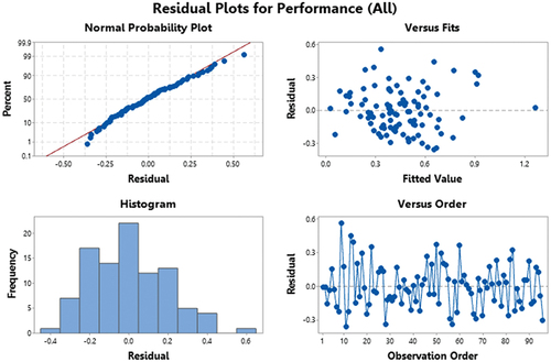
Having obtained these regression models, the error assumptions are then investigated. For demonstration, Figure 3 is used to verify the error assumptions of the multiple regression model for one year before becoming public firms. All error assumptions, including normal distribution, constant variance and independence are verified, and the model is determined to be valid. The results also apply to other models in other years. Furthermore, a lack-of-fit test is performed to check whether the terms in the models are sufficient to explain the firm financial performance or not. Since the p-value of every model is higher than 0.05 (the significance level), indicating that there is no evidence of lack of fit, it can be concluded that all prediction models are significant.

Figure 3. Error assumptions of the multiple regression model for one year before becoming public firms.

To measure the efficiency of the model, Mean Absolute Percentage Error (MAPE) is introduced. MAPE can be calculated in Equation 9(9) $\mathit{MAPE}=\frac{1}{n}\sum _{\mathit{t}=1}^n\left|\frac{A_t-F_t}{A_t}\right|$(9) , as follows:

(9) $\mathit{MAPE}=\frac{1}{n}\sum _{\mathit{t}=1}^n\left|\frac{A_t-F_t}{A_t}\right|$(9)

The lower value of MAPE indicates the higher accuracy of the prediction model. As suggested by Lewis (1982), the model is considered to be highly accurate if the MAPE value is less than 10%. If the MAPE value is between 10% and 20%, the model can provide a good prediction. If the MAPE value is between 20% and 50%, the model can produce a reasonable prediction. However, if the MAPE value is higher than 50%, the model is considered to be inaccurate and should not be used. The MAPE values of each multiple regression model are shown in Table 7. All prediction models have the values of MAPE within a range of 20% to 50% indicating that the efficiency of every model is acceptable.

Table 7. MAPE of each multiple regression model

Relative Year	MAPE
One year before	42.28%
One year after	48.96%
Two years after	45.16%
Three years after	49.04%
Four years after	48.47%

Although the multiple regression model can provide a detailed prediction with the actual value of firm financial performance, the accuracy of these model predictions is just acceptable and on the edge to be considered as inaccurate. As a result, another statistical technique, logistic regression, is then employed to make a similar prediction, but the scale of the prediction will be less (as a relative group rather than an actual scale) to bring up its accuracy.

4.2.2. Logistic regression

In the logistic regression, financial data are also analyzed using Minitab 19. Unlike multiple regression, three scenarios were considered. In the first scenario, the firms are divided into two groups, including a high and low performance group, by using the median of the combination of ROA, ROE and ROS as a threshold point. In the second scenario, the firms are divided into three groups, including a high, medium and low performance group, by using the 33^th and 66^th percentiles of the combination of ROA, ROE and ROS as threshold points. In the third scenario, the firms are divided into four groups, including a very high, high, low and very low performance group, by using the 25^th, 50^th and 75^th percentiles of the combination of ROA, ROE and ROS as threshold points. Binary logistic regression is applied in the first scenario, while ordinal logistic regression is applied in the last two scenarios. Similar aforementioned independent variables were used. Interactions among variables are allowed up to the second degree. Having applied the backward elimination method, the terms that have p-value exceeding 0.10 were eliminated from the model. Equations 10(10) $p_1=\frac{e^{-43.91+0.76X_1-13.28X_2-135.12X_3-15.37X_4-87.72X_5-2.34X_6-1.58X_1{X}_4+13.57X_2{X}_3+19.92X_3{X}_5-6.62X_3{X}_5-2.44X_4{X}_5+0.81X_4{X}_6+3.35X_5{X}_6}}{1+e^{-43.91+0.76X_1-13.28X_2-135.12X_3-15.37X_4-87.72X_5-2.34X_6-1.58X_1{X}_4+13.57X_2{X}_3+19.92X_3{X}_5-6.62X_3{X}_5-2.44X_4{X}_5+0.81X_4{X}_6+3.35X_5{X}_6}}$(10) to 19 present the final logistic regression model in each relative year of the second scenario (three-group) that will later be used in this study for demonstrating the application of the proposed financial performance prediction tool.

The logit model of the second scenario (three-group), one year before becoming public firms

(10) $p_1=\frac{e^{-43.91+0.76X_1-13.28X_2-135.12X_3-15.37X_4-87.72X_5-2.34X_6-1.58X_1{X}_4+13.57X_2{X}_3+19.92X_3{X}_5-6.62X_3{X}_5-2.44X_4{X}_5+0.81X_4{X}_6+3.35X_5{X}_6}}{1+e^{-43.91+0.76X_1-13.28X_2-135.12X_3-15.37X_4-87.72X_5-2.34X_6-1.58X_1{X}_4+13.57X_2{X}_3+19.92X_3{X}_5-6.62X_3{X}_5-2.44X_4{X}_5+0.81X_4{X}_6+3.35X_5{X}_6}}$(10)

(11) $p_2=\frac{e^{-41.87+0.76X_1-13.28X_2-135.12X_3-15.37X_4-87.72X_5-2.34X_6-1.58X_1{X}_4+13.57X_2{X}_3+19.92X_3{X}_5-6.62X_3{X}_5-2.44X_4{X}_5+0.81X_4{X}_6+3.35X_5{X}_6}}{1+e^{-41.87+0.76X_1-13.28X_2-135.12X_3-15.37X_4-87.72X_5-2.34X_6-1.58X_1{X}_4+13.57X_2{X}_3+19.92X_3{X}_5-6.62X_3{X}_5-2.44X_4{X}_5+0.81X_4{X}_6+3.35X_5{X}_6}}$(11)

where: $p_1$ is the probability to be predicted in a low performance group

$p_2$ is the probability to be predicted in low or medium performance groups

The logit model of the second scenario (three-group), 1^st year after becoming public firms

(12) $p_1=\frac{e^{6.86-1.69X_1-6.17X_2-9.70X_3-2.85X_4-8.90X_5-0.29X_6-1.63X_1{X}_2+6.56X_1{X}_3-3.70X_1{X}_4-2.21X_1{X}_5-7.00X_2{X}_4-5.15X_2{X}_5+8.54X_3{X}_4-6.38X_4{X}_5}}{1+e^{6.86-1.69X_1-6.17X_2-9.70X_3-2.85X_4-8.90X_5-0.29X_6-1.63X_1{X}_2+6.56X_1{X}_3-3.70X_1{X}_4-2.21X_1{X}_5-7.00X_2{X}_4-5.15X_2{X}_5+8.54X_3{X}_4-6.38X_4{X}_5}}$(12)

(13) $p_1=\frac{e^{9.25-1.69X_1-6.17X_2-9.70X_3-2.85X_4-8.90X_5-0.29X_6-1.63X_1{X}_2+6.56X_1{X}_3-3.70X_1{X}_4-2.21X_1{X}_5-7.00X_2{X}_4-5.15X_2{X}_5+8.54X_3{X}_4-6.38X_4{X}_5}}{1+e^{9.25-1.69X_1-6.17X_2-9.70X_3-2.85X_4-8.90X_5-0.29X_6-1.63X_1{X}_2+6.56X_1{X}_3-3.70X_1{X}_4-2.21X_1{X}_5-7.00X_2{X}_4-5.15X_2{X}_5+8.54X_3{X}_4-6.38X_4{X}_5}}$(13)

where: $p_1$ is the probability to be predicted in a low performance group

$p_2$ is the probability to be predicted in low or medium performance groups

The logit model of the second scenario (three-group), 2^nd year after becoming public firms

(14) $p_1=\frac{e^{-0.39+0.91X_1+4.51X_2-3.79X_3+2.10X_4-8.52X_5-0.03X_6-1.01X_1{X}_2-1.29X_1{X}_4-11.17X_2{X}_5+21.38X_3{X}_5-1.96X_4{X}_5}}{1+e^{-0.39+0.91X_1+4.51X_2-3.79X_3+2.10X_4-8.52X_5-0.03X_6-1.01X_1{X}_2-1.29X_1{X}_4-11.17X_2{X}_5+21.38X_3{X}_5-1.96X_4{X}_5}}$(14)

(15) $p_2=\frac{e^{1.51+0.91X_1+4.51X_2-3.79X_3+2.10X_4-8.52X_5-0.03X_6-1.01X_1{X}_2-1.29X_1{X}_4-11.17X_2{X}_5+21.38X_3{X}_5-1.96X_4{X}_5}}{1+e^{1.51+0.91X_1+4.51X_2-3.79X_3+2.10X_4-8.52X_5-0.03X_6-1.01X_1{X}_2-1.29X_1{X}_4-11.17X_2{X}_5+21.38X_3{X}_5-1.96X_4{X}_5}}$(15)

where: $p_1$ is the probability to be predicted in a low performance group

$p_2$ is the probability to be predicted in low or medium performance groups

The logit model of the second scenario (three-group), 3^rd year after becoming public firms

(16) $p_1=\frac{e^{12.31+5.14X_1-10.69X_2-10.53X_3-14.19X_4-12.92X_5-0.01X_6-0.25X_1{X}_6+10.83X_2{X}_3+14.65X_3{X}_4+15.41X_3{X}_5}}{1+e^{12.31+5.14X_1-10.69X_2-10.53X_3-14.19X_4-12.92X_5-0.01X_6-0.25X_1{X}_6+10.83X_2{X}_3+14.65X_3{X}_4+15.41X_3{X}_5}}$(16)

(17) $p_2=\frac{e^{14.54+5.14X_1-10.69X_2-10.53X_3-14.19X_4-12.92X_5-0.01X_6-0.25X_1{X}_6+10.83X_2{X}_3+14.65X_3{X}_4+15.41X_3{X}_5}}{1+e^{14.54+5.14X_1-10.69X_2-10.53X_3-14.19X_4-12.92X_5-0.01X_6-0.25X_1{X}_6+10.83X_2{X}_3+14.65X_3{X}_4+15.41X_3{X}_5}}$(17)

where: $p_1$ is the probability to be predicted in a low performance group

$p_2$ is the probability to be predicted in low or medium performance groups

The logit model of the second scenario (three-group), 4^th year after becoming public firms

(18) $p_2=\frac{e^{156.69-8.97X_1-6.29X_2-173.04X_3-13.96X_4-1.74X_5-7.14X_6-1.93X_1{X}_2-1.45X_1{X}_4+0.47X_1{X}_6-7.86X_3{X}_4-21.27\mathit{X}{X}_3{X}_4+7.81X_3{X}_6}}{1+e^{156.69-8.97X_1-6.29X_2-173.04X_3-13.96X_4-1.74X_5-7.14X_6-1.93X_1{X}_2-1.45X_1{X}_4+0.47X_1{X}_6-7.86X_3{X}_4-21.27\mathit{X}{X}_3{X}_4+7.81X_3{X}_6}}$(18)

(19) $p_2=\frac{e^{159.11-8.97X_1-6.29X_2-173.04X_3-13.96X_4-1.74X_5-7.14X_6-1.93X_1{X}_2-1.45X_1{X}_4+0.47X_1{X}_6-7.86X_3{X}_4-21.27\mathit{X}{X}_3{X}_4+7.81X_3{X}_6}}{1+e^{159.11-8.97X_1-6.29X_2-173.04X_3-13.96X_4-1.74X_5-7.14X_6-1.93X_1{X}_2-1.45X_1{X}_4+0.47X_1{X}_6-7.86X_3{X}_4-21.27\mathit{X}{X}_3{X}_4+7.81X_3{X}_6}}$(19)

where: $p_1$ is the probability to be predicted in a low performance group

$p_2$ is the probability to be predicted in low or medium performance groups

During the process of developing these logistic regression models, the goodness-of-fit tests are performed to verify whether the independent variables used in the model (liquidity, leverage, COGS, asset utilization, tangibility and company size) are sufficient or not. Using a significance level of 0.05, the p-value of each model is higher than the significance level. Therefore, it can be concluded that all prediction models are significant under a 95% confident level.

These logistic regression models provide the probability of the firms to be in each group. The group that has the highest probability will indicate the predicted outcome. For example, if firm M has a probability of 10%, 30% and 60% to be in a low, medium and high performance group, respectively, firm M will be predicted in the high performance group. To evaluate the efficiency of the model, the accuracy rate is also introduced. The accuracy rate can be measured by determining the rate to which the outcome of the model is exactly matched with the actual value. In this case, if a firm is classified as a high performance firm and this firm is actually a high performance firm, the accuracy becomes 100%. On the other hand, if a firm is classified as a high performance firm and this firm is actually a low performance firm, the accuracy becomes 0%. By averaging the accuracy of all firms, the accuracy of the model can be achieved. Table 8 presents the accuracy rates of each logistic regression model.

Table 8. Accuracy rates of logistic models

Relative Year	2-group	3-group	4-group
One year before	78.95%	61.05%	58.95%
One year after	80.00%	63.00%	52.00%
Two years after	74.03%	59.74%	44.16%
Three years after	89.25%	65.59%	52.69%
Four years after	78.57%	69.05%	64.29%
Average	80.16%	63.69%	54.42%

According to Table 8, the average accuracy rate for the two-group model is 80.16%, while the average accuracy rate for the three-group model is 63.69%, and the average accuracy rate for the four-group model is 54.42%. By comparing these three models, the prediction model with less possible outcomes (the two-group model) will certainly provide a higher accuracy rate. Furthermore, when comparing the multiple regression model that employs the interval response and the logistic regression model that employs the categorical response, the logistic regression model outperforms in terms of accuracy, while the multiple regression model is superior in terms of a detailed prediction with an individual scale. Therefore, logistic regression is suggested if the prediction requires a high accuracy, while multiple regression is suggested if the prediction requires the exact predicted value. Among the prediction models that are developed, the three-group logistic regression model is selected to be used in this study for further analysis since the predicted outcomes are not too bad and the accuracy is acceptable (average of 63.69%), whereas the predicted outcomes of the two-group model (yes or no) are too limited and the four-group model’s accuracy is too low.

For further investigation, the effect of an individual factor (independent variable) on the firm financial performance (dependent variable) is explored using the selected three-group logistic regression model. To clarify, in the model, the predicted outcome can be one of the following: a high performance group (Q1), a medium performance group (Q2) and a low performance group (Q3). Since the model includes the interactions between any two factors, the effect of each factor is difficult to interpret through the equations. Therefore, to overcome this difficulty, three scenarios are presented to investigate how each factor is related to the performance. The first scenario is for firm A that is predicted to be in the high performance group (Q1) in any relative transition years. The second scenario is for firm B that is predicted to be in the medium performance group (Q2) in any relative transition years. The last scenario is for firm C that is predicted to be in the low performance group (Q3) in any relative transition years.

The status of the firm in each scenario is shown in Table 9. The investigation in each scenario is done by gradually changing the value of only the interested factor while leaving the rest factors the same and observing how the predicted firm performance and its status change in relation to the other firms in the market. A certain range for variation of each factor is determined according to the recommended value or the nature of each factor as shown in Table 10. The results of the investigation on the effect of the individual factor are shown in Figures 4-9. The highlighted columns in circle number 1 in these figures indicate the initial status of the firm in each scenario before adjusting the value of the factor. The unhighlighted cells indicate that the firm is still predicted to be in the same group as it is at the beginning (same as the highlighted cells in the circle number 1). The highlighted cells in circle number 2 indicate that the firm is predicted to be in an inferior performance group. For example, at a specific value of a specific factor, if the highlighted cells in circle number 2 are from firm B, it indicates that firm B will be predicted to be in a low performance group (Q3). As shown in Figure 4, in the fourth year after going public, the highlighted cells in circle number 2 cover the level of liquidity from 0 to 0.4 meaning that firm B will be predicted to be in a low performance group (Q3) if the level of liquidity is lower than or equal to 0.4. On the other hand, the highlighted cells in circle number 3 indicate that the firm is predicted to be in a better performance group. For example, at a specific value of a specific factor, if the highlighted cells in circle number 3 are from firm B, it indicates that firm B will be predicted to be in a high performance group (Q1). According to Figure 4, in the fourth year after going public, the highlighted cells in circle number 3 cover the level of liquidity from 2.1 to 3 meaning that firm B will be predicted to be in a high performance group (Q1) if the level of liquidity is higher than or equal to 2.1. The explanation of the results will then be given. It should be noted that different results may be achieved if the firm with a different initial status is considered. However, if this firm is predicted to be in the same group as in one of the three scenarios, for instance, it is predicted to be in Q1, the obtained results will be similar to the results from the first scenario. In addition, it should also be noted that the prediction results are subject to certain accuracy rates as presented in Table 8 as the prediction is not always 100% accurate.

Figure 4. The impact of liquidity on predicted performance.

Figure 5. The impact of leverage on predicted performance.

Figure 6. The impact of COGS on predicted performance.

Figure 7. The impact of asset utilization on predicted performance.

Figure 8. The impact of tangibility on predicted performance.

Figure 9. The impact of company size on predicted performance.

Table 9. Status of the firm in each scenario

Factors	Firms
	A	B	C
Liquidity	1.7	1.2	0.7
Leverage	0.9	0.7	0.5
COGS	0.7	0.8	0.9
Asset Utilization	0.9	0.7	0.5
Tangibility	0.9	0.7	0.5
Company Size	23	22	21

Table 10. Range variation of each factor

Variation Range
Liquidity	0–3
Leverage	0–1
COGS	0–1
Asset Utilization	0–1
Tangibility	0–1
Company Size	20–25

Regarding the variation of liquidity in Figure 4, the firms in every scenario seem to have a similar trend. If liquidity increases, the firms will have a higher probability to be predicted to be in a better group. In contrast, if liquidity decreases, the firms will have a higher probability to be predicted to be in an inferior group. The specific value of liquidity that results in the change of the predicted performance can be observed. For example, at the first year after becoming listed, firm B will be predicted to be in Q3 (an inferior performance group) if liquidity is lower than or equal to 0.5 (see circle number 4). On the other hand, firm B will be predicted to be in Q1 (a better performance group) if liquidity is higher than or equal to 1.9. The results suggest that in the second year after becoming listed, if a medium performance firm such as firm B wants to position itself in Q1 (having a better performance compared to other firms), it has to increase liquidity to be at least 1.9 from the initial value of 1.2 (under the condition that the other variables remain the same).

Considering the variation of leverage in Figure 5, a similar trend can be found between firm A and firm B. By decreasing the level of leverage, the firm will have a higher probability to be predicted to be in an inferior group. On the other hand, increasing the level of leverage cannot increase enough probability to change the value of their predicted performance to be in a better group. It is suggested that high and medium performance firms such as firm A and firm B should not focus on increasing the level of leverage, but they should focus on preventing the reduction of leverage. The specific values of the leverage that affect the predicted performance can also be found. For instance, firm A will be predicted to be in Q2 (an inferior performance group) if the firm reduces its level of leverage to be lower than or equal to 0.4 from the initial value of 0.9 (see circle number 4) at the third year after going public. For a low performance firm such as firm C, unlike the first two firms, changing the level of leverage seems to have no effect on firm C’s performance. It is recommended that firm C ignores any activities related to the change in the level of leverage.

Opposite to other factors, COGS and the performance of the three firms are not positively correlated with each other. Decreasing the level of COGS can improve the firm financial performance, while increasing the level of COGS can worsen the predicted performance. As shown in Figure 6, at the fourth year after going public, firm B, which is initially predicted to be in Q2 (a medium performance group), will be predicted to be in Q1 or a better group if it can reduce the level of COGS to be at least 0.7 (from the initial value of 0.8). In contrast, firm B will be predicted to be in Q3 or an inferior group if the level of COGS increases to be at least 0.9 (see circle number 4). To achieve a better performance, it is suggested that COGS should be reduced.

According to Figure 7, asset utilization seems to have the same impact on firm performance as leverage does. Increasing the level of asset utilization cannot change the predicted performance of firm A or firm B, while the predicted performance of these firms can be worse if the level of asset utilization is reduced. It is recommended that high and medium performance firms such as firm A and firm B should prevent a decrease in asset utilization. As suggested in Figure 7, at the fourth year after going public, firm A should maintain a level of asset utilization to be higher than 0.4 from the initial value of 0.9 (see circle number 4) to prevent an inferior outcome, which is the predicted performance in Q2 (an inferior performance group). On the other hand, asset utilization seems to have no impact on firm C’s performance. It should be eliminated from the list of interested factors for low performance firms such as firm C.

Similar to leverage and asset utilization, as shown in Figure 8, the predicted performances of firm A and firm B are affected only by the decrease in tangibility. The probability of these firms to be predicted in inferior groups will be higher if the level of tangibility is lower. At the second year after becoming public, firm A can be predicted to be in Q2 (a medium performance group) if the level of tangibility is managed to be lower than or equal to 0.2 (see circle number 4). Other specific values of tangibility that result in changes of predicted performance can be noticed according to Figure 8. For a low performance firm such as firm C, its performance is not affected by the change of tangibility. Thus, tangibility is suggested to be ignored in this scenario.

Regarding Figure 9, the company size seems to have no impact on the performance of high and low performance firms such as firm A and firm B. It is recommended that these two firms should not consider changing the level of the company size if they would like to improve their firm relative financial performance. However, for a low performance firm such as firm C, increasing the level of the company size can increase the probability that its predicted relative performance will be better. For example, at the first year after going public, if firm C can increase the level of the company size to be higher than 23.5 (see circle number 4), it can be predicted to be in Q2, which is a better group of performance. It is suggested that firm C can focus on increasing the company size at the early year during the transition period of becoming public in order to improve its relative financial performance as compared to other firms in the market.

5. Managerial implication

In this section, a small example case is introduced to demonstrate another application and benefit of the financial performance prediction model. Assuming that firm Z recently joined the stock market, the current financial data of firm Z is shown in Table 11. In the first year after becoming public, the firm wants to expand its production capacity by buying new machines that are worth 400 million baht (1US$ ≈ 34 baht) in total. According to its managers’ decision, instead of using its own money, they decide to utilize a bank loan with an interest rate of 10% so that an interest of 40 million baht will be paid at the end of the year. The financial performance prediction model can be used to check whether this investment is worth doing or not. Furthermore, if it is not worth doing, how it can be made worthwhile. This is to find out the most effective investment plan of when and how much should be invested.

Table 11. Financial data of firm Z

Source	Financial Data	Value (million baht)
Selected data from the balance sheet	Current Assets	700
	Non-current Assets	1,000
	Total Assets	1,700
	Current Liabilities	600
	Non-current Liabilities	300
	Total Liabilities	900
Selected data from the income statement	Sales	1,000
	Cost of Goods Sold	800

Assuming that the firm wants to make the investment in the first year after going public, Equations 12(12) $p_1=\frac{e^{6.86-1.69X_1-6.17X_2-9.70X_3-2.85X_4-8.90X_5-0.29X_6-1.63X_1{X}_2+6.56X_1{X}_3-3.70X_1{X}_4-2.21X_1{X}_5-7.00X_2{X}_4-5.15X_2{X}_5+8.54X_3{X}_4-6.38X_4{X}_5}}{1+e^{6.86-1.69X_1-6.17X_2-9.70X_3-2.85X_4-8.90X_5-0.29X_6-1.63X_1{X}_2+6.56X_1{X}_3-3.70X_1{X}_4-2.21X_1{X}_5-7.00X_2{X}_4-5.15X_2{X}_5+8.54X_3{X}_4-6.38X_4{X}_5}}$(12) and 13(13) $p_1=\frac{e^{9.25-1.69X_1-6.17X_2-9.70X_3-2.85X_4-8.90X_5-0.29X_6-1.63X_1{X}_2+6.56X_1{X}_3-3.70X_1{X}_4-2.21X_1{X}_5-7.00X_2{X}_4-5.15X_2{X}_5+8.54X_3{X}_4-6.38X_4{X}_5}}{1+e^{9.25-1.69X_1-6.17X_2-9.70X_3-2.85X_4-8.90X_5-0.29X_6-1.63X_1{X}_2+6.56X_1{X}_3-3.70X_1{X}_4-2.21X_1{X}_5-7.00X_2{X}_4-5.15X_2{X}_5+8.54X_3{X}_4-6.38X_4{X}_5}}$(13) from the logit model must be used. At the beginning, firm Z’s performance will be predicted using the current status. Then, the status will be changed in relation to the above-mentioned situation, and firm Z’s financial performance will be predicted again using this new status. The results will then be compared, and suggestions will be made.

Starting with the prediction using the current financial status of firm Z. Prior to the analysis, the values of required factors are calculated and presented in Table 12. Having obtained the factors, the relative performance prediction can be made. The result reveals that firm Z is predicted to be in Q3 or a low performance group.

Table 12. Status of firm Z

Factors	Values
Liquidity	1.167
Leverage	0.529
COGS	0.8
Asset Utilization	0.588
Tangibility	0.588
Company Size	21.254

Then, due to such an investment, the financial structure of firm Z will be changed. Non-current liabilities and total liabilities will be increased by 400 million baht resulting from the bank loan. Non-current assets will also be increased by 400 million baht as a consequence of factory expansion and purchasing machines. Cash, which is a part of current assets, will be reduced by 40 million baht due to the interest of the bank loan. Tables 13 and 14 present the consequence of the financial data and status of firm Z after this investment. From the prediction with this financial data, the result shows that firm Z is still predicted to be in Q3 or in a low performance group. The reason behind this outcome is that the firm just bought new machines and expanded its factory, but it does not have any financial benefit from such actions yet as the sales still remain the same.

Table 13. Financial data of firm Z after the investment

Source	Financial Data	Value (million baht)
Selected data from the balance sheet	Current Assets	660
	Non-current Assets	1,400
	Total Assets	2,060
	Current Liabilities	600
	Non-current Liabilities	700
	Total Liabilities	1,300
Selected data from the income statement	Sales	1,000
	Cost of Goods Sold	800

Table 14. Status of firm Z after the investment

Factors	Values
Liquidity	1.1
Leverage	0.631
COGS	0.8
Asset Utilization	0.485
Tangibility	0.679
Company Size	21.445

To make this investment worthwhile, more sales need to be generated. Assuming that the sales and the cost of goods sold increase in the same proportion as their past ratio before the investment, the changing financial data and status of firm Z through experimenting with an increase in sales and cost of goods sold are shown in Tables 15 and 16.

Table 15. Financial data of firm Z after the investment and the increase in sales

Source	Financial Data	Value (million Baht)
Selected data from the balance sheet	Current Assets	660
	Non-current Assets	1,400
	Total Assets	2,060
	Current Liabilities	600
	Non-current Liabilities	700
	Total Liabilities	1,300
Selected data from the income statement	Sales	1,300
	Cost of Goods Sold	1,040

Table 16. Status of firm Z after the investment and the increase in sales

Factors	Values
Liquidity	1.1
Leverage	0.631
COGS	0.8
Asset Utilization	0.631
Tangibility	0.679
Company Size	21.445

According to the results from the financial performance prediction model, firm Z will now be predicted to be in Q2 or in a medium performance group (a better group) if it can increase sales to be at least 1,300 million baht (30% increase). By knowing that the investor can realize that this investment will only be worth enough to upgrade its relative financial performance as compared to others in the market when it must increase its sales by 30%. However, this result is subject to a year of the prediction. For example, in order to upgrade its relative performance, firm Z must increase at least 300 million baht of sales in that investing year. In reality, this new expansion may not have an immediate effect in that year, so the model of other years can be employed and experimented with this new status so that the worthiness of this investment can be observed in other years. Please also note that this prediction is subject to the accuracy rates of the prediction model as presented in Table 8, and it is a sole result of one business decision as many business actions can happen at the same time in reality.

6. Financial performance prediction tool

Due to the complexity of the logistic regression equations and the amount of data involved, performing the experiment on the prediction model by hand is very inconvenient and time-consuming. To obtain the predicted outcome, many steps need to be done as illustrated in the previous section. Users must find the financial data, calculate the required factor, calculate the probability of each outcome, and determine what the predicted outcome is. As a result, a more user-friendly tool is introduced to help the managers or decision makers effectively utilize the prediction model. This tool is called the financial performance prediction tool. It was developed in Microsoft Excel with its macro. The tool includes two important parts, namely input and output. The input part is for filling in essential current financial data, including selected data from balance sheet (current assets, non-current assets, total assets, current liabilities, non-current liabilities and total liabilities) and selected data from income statement (sales and cost of goods sold) as shown in Figure 10. These data will be fed into the logistic regression model for calculating the relative financial performance. The prediction results will be presented in the output part as shown in Figure 11. This part provides the calculated value of each factor, the probability to be predicted in each group of performance in each year, the predicted group of performance and the effect from varying each individual factor according to the input financial data.

Figure 10. The financial performance prediction tool (input part).

Figure 11. The financial performance prediction tool (output part).

The users can input the financial data of their firms directly without calculating the value of factors or the probability of each outcome. The prediction tool will then perform all the calculations automatically and provide the predicted outcome in a specified year. The factors and the financial performances that should be emphasized can be observed. Furthermore, the users can use the results of the prediction to prepare the most effective investment plan of when and how much should be invested. For example, if the users want to expand their production capacity, they can try predicting the relative performance in different years to find what year is the best year for the expansion. On the other hand, if the expansions are planned in a specific year, the users can try to experiment by changing the values of their determinants through their financial statements to find out how to benefit most from such an expansion as demonstrated in the previous sections.

7. Conclusions

This study aimed to develop a financial performance prediction model using the logistic regression technique based on listed firms in the SET during the transition period of going public.

The analysis was based on two internal capability determinants, namely Firm Financial Strength (Liquidity, Leverage and Cost of Goods Sold) and Firm Characteristics (Asset Utilization, Tangibility and Company Size). The results indicated that the multiple regression method was not suitable for such a prediction as the logistic regression method outperformed in terms of prediction accuracy. By weighing the benefits and drawbacks, the logistic regression model for predicting three groups of firm performance (combination of ROA, ROE and ROS) with the average accuracy of 63.69% was selected for further analysis.

The main experiment was then carried out in three steps. In the first step (as presented in the results and discussion), the varying effect of each factor was investigated. The investigation in each scenario was done by gradually changing the value of only the interested factor while leaving the rest factors the same and observing how the predicted firm performance and its status change in relation to the other firms in the market. The findings presented that liquidity had a positive relationship to the firm performance. High level of current assets could lead to a high firm financial performance. As opposed to liquidity, COGS revealed a negative relationship to the firm performance. To achieve a better performance, the firms should try to keep the level of COGS low. For leverage, asset utilization and tangibility, increasing the levels of these factors had no impact on firm performance, while decreasing the levels of these factors could harm the performance of high and medium performance firms. In contrast, reducing the level of the company size seemed to have to effect on firm performance, but increasing the level of the company size could benefit the performance of low performance firms.

In addition to discovering the effects of each factor, the experiment in the second step involved the managerial implication where the managerial benefit of the financial performance prediction model was demonstrated. If the firm wants to make an investment by a certain way of business transactions, the prediction model can be used to confirm whether such an investment is worthwhile or not (in terms of upgrading its relative financial performance). If it is not worthwhile, the model can help identify how to make it worthwhile. It can provide the recommendations (e.g., when and how much to invest) for achieving a better performance to the firms during this transition period.

Next, due to the complexity of the logistic regression equations and the amount of data involved, performing the experiment on the prediction model by hand is very inconvenient and time-consuming, and the financial performance prediction tool was developed to help managers or decision makers effectively utilize the obtained logistic regression model. The users can repeatedly use the tool based on the developed model to find the recommendations or strategies for achieving a better financial performance. So, it can become an important assistant to deal with business decisions.

In this study, several limitations can be reached. First of all, the analysis was performed based on the financial data in the SET. Due to the uniqueness of Thai firms, the results of this study are not generalized for any countries. Secondly, the financial performance prediction model was developed by including the financial data of all firms in the market. The characteristics of each industry in the market cannot be extracted. Future researches may consider developing the prediction performance for each industry. Thirdly, according to the analysis, the success of the firm is determined by the relative financial performance. Different outcomes can be achieved if different indicators of success are measured. Fourth, the prediction model includes only internal capability determinants, namely firm financial strengths and firm characteristics. Other external determinants such as form or supply chain cooperation, innovation, socio-economic and cultural environment factors can also be considered. Another limitation is that the prediction tool is based on the logistic regression model. Other methods of prediction using Artificial Intelligent, such as machine learning, may be considered. This can help improve the accuracy of the prediction model. Finally, the effects of internal determinants are investigated based on a case of three example firms. If other firms that have a different status from the example firms are considered, different results may be obtained. However, this can easily be done with the developed financial performance prediction tool.

Correction

This article has been corrected with minor changes. These changes do not impact the academic content of the article.

Disclosure statement

No potential conflict of interest was reported by the authors.

Additional information

Funding

The work was supported by the Thammasat University Research Fund [Contract Number: TUFT 33/2566}.

References

- Ablanedo-Rosas, J. H., Gao, H., Zheng, X., Alidaee, B., & Wang, H. (2010). A study of the relative efficiency of Chinese ports: A financial ratio-based data envelopment analysis approach. Expert Systems, 27(5), 349–28. https://doi.org/10.1111/j.1468-0394.2010.00552.x
- Abor, J. (2005). The effect of capital structure on profitability: An empirical analysis of listed firms in Ghana. The Journal of Risk Finance, 6(5), 438–445. https://doi.org/10.1108/15265940510633505
- Aburisheh, K. E., Dahiyat, A. A., & Owais, W. O. (2022). Impact of cash flow on earnings management in Jordan. Cogent Business & Management, 9(1), 2135211. https://doi.org/10.1080/23311975.2022.2135211
- Ahmed, N., & Afza, T. (2019). Capital structure, competitive intensity and firm performance: Evidence from Pakistan. Journal of Advances in Management Research, 16(5), 796–813. https://doi.org/10.1108/jamr-02-2019-0018
- Ahmed, N., Ahmad, Z., & Ahmed, I. (2010). Determinants of capital structure: A case of life insurance sector of Pakistan. European Journal of Economics Finance and Administrative Sciences, 24, 7–12.
- Akoglu, H. (2018). User’s guide to correlation coefficients. Turkish Journal of Emergency Medicine, 18(3), 91–93. https://doi.org/10.1016/j.tjem.2018.08.001
- Almajali, A. Y., Alamro, S. A., & Al-Soub, Y. Z. (2012). Factors affecting the financial performance of Jordanian insurance companies listed at amman stock exchange. Journal of Management Research, 4(2), 266–289. https://doi.org/10.5296/jmr.v4i2.1482
- Altaf, N., & Shah, F. A. (2018). How does working capital management affect the profitability of Indian companies? Journal of Advances in Management Research, 15(3), 347–366. https://doi.org/10.1108/jamr-06-2017-0076
- Babalola, Y. A. (2013). The effect of firm size on firms profitability in Nigeria. Journal of Economics & Sustainable Development, 4(5), 90–94.
- Banafa, A. S., Muturi, W., & Ngugi, K. (2015). The impact of leverage on financial performance of listed non-financial firm in Kenya. International Journal of Finance and Accounting, 4(7), 1–20.
- Bătae, O. M., Dragomir, V. D., & Feleagă, L. (2021). The relationship between environmental, social, and financial performance in the banking sector: A European study. Journal of Cleaner Production, 290, 125791. https://doi.org/10.1016/j.jclepro.2021.125791
- Bongoye, M. G., Banafa, A., & Kingi, W. (2016). Effect of firm specific factors on financial performance of non-financial firms listed at nairobi securities exchange. Imperial Journal of Interdisciplinary Research, 2(12), 253–265.
- Bose, I., & Pal, R. (2006). Predicting the survival or failure of click-and-mortar corporations: A knowledge discovery approach. European Journal of Operational Research, 174(2), 959–982. https://doi.org/10.1016/j.ejor.2005.05.009
- Cochran, P. L., & Wood, R. A. (1984). Corporate social responsibility and financial performance. Academy of Management Journal, 27(1), 42–56. https://doi.org/10.2307/255956
- Dagestani, A. A., & Qing, L. (2022). The impact of environmental information disclosure on Chinese firms’ environmental and economic performance in the 21st century: A systematic review. IEEE Engineering Management Review, 50(4), 203–214. https://doi.org/10.1109/EMR.2022.3210465
- Ellis, R. (1998). Asset utilization: A metric for focusing reliability efforts (7th Ed.). Westside Houston.
- Eva, H., & Roman, S. (2018). Return on sales and wheat yields per hectare of European agricultural entities. Agricultural Economics, 64(10), 436–444. https://doi.org/10.17221/209/2017-agricecon
- Fazlzadeh, A., Hendi, A. T., & Mahboubi, K. (2011). The examination of the effect of ownership structure on firm performance in listed firms of Tehran stock exchange based on the type of the industry. International Journal of Business & Management, 6(3), 249–267. https://doi.org/10.5539/ijbm.v6n3p249
- Flamini, C., Valentina, C., McDonald, G., & Liliana, S. (2009). The determinants of commercial Bank profitability in Sub-saharan Africa, Working Paper, IMF.
- Ghafoorifard, M., Sheykh, B., Shakibaee, M., & Joshaghan, N. S. (2014). Assessing the relationship between firm size, age and financial performance in listed companies on tehran stock exchange. International Journal of Scientific Management and Development, 2(3), 631–635.
- Ghosh, S. (2008). Leverage, foreign borrowing and corporate performance: Firm-level evidence for India. Applied Economics Letters, 15(8), 607–616. https://doi.org/10.1080/13504850600722047
- Harvey, C. R., Lins, K. V., & Roper, A. H. (2001). The effect of capital structure when expected agency costs are extreme. Journal of Financial Economics, 74(1), 3–30. https://doi.org/10.1016/j.jfineco.2003.07.003
- He, B., Ma, X., Malik, M. N., Shinwari, R., Wang, Y., Qing, L., Dagestani, A. A., & Ageli, M. M. (2022). Sustainable economic performance and transition towards cleaner energy to mitigate climate change risk: Evidence from top emerging economies. Economic Research-Ekonomska Istraživanja, 36(3). https://doi.org/10.1080/1331677x.2022.2154240
- Hensher, D. A., Jones, S., & Greene, W. H. (2007). An error component logit analysis of corporate bankruptcy and insolvency risk in Australia. The Economic Record, 83(260), 86–103. https://doi.org/10.1111/j.1475-4932.2007.00378.x
- Hvide, H., & Møen, J. (2007). Liquidity constraints and entrepreneurial performance. Department of Business and Management Science, Norwegian School of Economics.
- Jensen, M. C., & Meckling, W. H. (1976). Theory of the firm: Managerial behaviour, agency costs and ownership structure. Journal of Financial Economics, 3(4), 305–360. https://doi.org/10.1016/0304-405X(76)90026-X
- Kabajeh, M. A. M., Aimat, S. M. A., & Dahmash, F. N. (2012). The relationship between the ROA, ROE and ROI ratios with jordanian insurance public companies market share prices. International Journal of Humanities and Social Science, 2(11), 115–120.
- Kelley, K., Bolin, J., & H, H. (2013). Multiple Regression. In T. Teo (Ed.), Handbook of quantitative methods for educational research (pp. 71–101). SensePublishers.
- Kim, C. -S., Mauer, D. C., & Sherman, A. E. (1998). The determinants of corporate liquidity: Theory and evidence. The Journal of Financial and Quantitative Analysis, 33(3), 335–359. https://doi.org/10.2307/2331099
- Krisnanto, J. (2016). How advertising intensity and promotion costs effect operating profit in four type Indonesian banking industry. Journal of Accounting & Marketing, 3(5), 1–5. https://doi.org/10.4172/2168-9601.1000181
- Lam, M. (2004). Neural network techniques for financial performance prediction: Integrating fundamental and technical analysis. Decision Support Systems, 37(4), 567–581. https://doi.org/10.1016/s0167-9236(03)00088-5
- Le Thi Kim, N., Duvernay, D., & Le Thanh, H. (2021). Determinants of financial performance of listed firms manufacturing food products in Vietnam: Regression analysis and Blinder–Oaxaca decomposition analysis. Journal of Economics and Development, 23(3), 267–283. https://doi.org/10.1108/jed-09-2020-0130
- Lewis, C. D. (1982). Industrial and business forecasting methods. Butterworths.
- Liargovas, P. G., & Skandalis, K. S. (2010). Factors affecting firms’ performance: The case of Greece. Global Business and Management Research An International Journal, 2(2), 184–197.
- Majumdar, S. K. (1997). The impact of size and age on firm-level performance: Some evidence from India. Review of Industrial Organization, 12(2), 231–241. https://doi.org/10.1023/A:1007766324749
- Mehari, D., & Aemiro, T. (2013). Firm-specific factors that determine insurance companies’ performance in Ethiopia. European Scientific Journal, 9(10), 245–255. 10.19044/esj.2013.v9n10p/p
- Muritala, T. A. (2012). An empirical analysis of capital structure on firm’s performance in Nigeria. International Journal of Advances in Management and Economics, 1(5), 116–124.
- Nasrallah, N., & El Khoury, R. (2022). Is corporate governance a good predictor of SMEs financial performance? Evidence from developing countries (the case of Lebanon). Journal of Sustainable Finance & Investment, 12(1), 13–43. https://doi.org/10.1080/20430795.2021.1874213
- Öğüt, H., Doğanay, M. M., & Ceylan, N. B. (2012). Prediction of bank financial strength ratings: The case of Turkey. Economic Modelling, 29(3), 632–640. https://doi.org/10.1016/j.econmod.2012.01.010
- Olson, D. L., Delen, D., & Meng, Y. (2012). Comparative analysis of data mining methods for bankruptcy prediction. Decision Support Systems, 52(2), 464–473. https://doi.org/10.1016/j.dss.2011.10.007
- Opler, T., Pinkowitz, L., Stulz, R., & Williamson, R. (1999). The determinants and implications of corporate cash holdings. Journal of Financial Economics, 52(1), 3–46. https://doi.org/10.1016/s0304-405x(99)00003-3
- Orlitzky, M., Schmidt, F. L., & Rynes, S. L. (2003). Corporate social and financial performance: A metaanalysis. Organization Studies, 24(3), 403–441. https://doi.org/10.1177/0170840603024003910
- Park, J. W., & Guahk, S. (2017). Financial performance of healthcare firms: The cases of Korea. International Journal of Economics and Financial Issues, 7(3), 721–728.
- Pasiouras, F., & Kosmidou, K. (2007). Factors influencing the profitability of domestic and foreign commercial banks in the European Union. Research in International Business and Finance, 21(2), 222–237. https://doi.org/10.1016/j.ribaf.2006.03.007
- Petersen, M. A., & Schoeman, I. (2008). Modeling of banking profit via return-on-assets and return-on-equity. Proceedings of the World Congress on Engineering, 2, 1–6.
- Rajan, R. G., & Zingales, L. (1995). What do we know about capital structure? Some evidence from international data. The Journal of Finance, 50(5), 1421–1460. https://doi.org/10.1111/j.1540-6261.1995.tb05184.x
- Ravi, V., Kurniawan, H., Thai, P. N. K., & Kumar, P. R. (2008). Soft computing system for bank performance prediction. Applied Soft Computing, 8(1), 305–315. https://doi.org/10.1016/j.asoc.2007.02.001
- Seema, G. P. K., & Surendra, S. Y. (2011). Impact of MOU on financial performance of public sector enterprises in India. Journal of Advances in Management Research, 8(2), 263–284. https://doi.org/10.1108/09727981111175984
- Sinthupundaja, J., & Chiadamrong, N. (2017). Investigating the determinants of Thai manufacturing public firms’ performance using an integration of multiple linear regression and hierarchical linear modelling. International Journal of Business Excellence, 11(2), 162–184. https://doi.org/10.1504/ijbex.2017.081430
- Teeratansirikool, L., Siengthai, S., Badir, Y., & Charoenngam, C. (2013). Competitive strategies and firm performance: The mediating role of performance measurement. International Journal of Productivity & Performance Management, 62(2), 168–184. https://doi.org/10.1108/17410401311295722
- Waddock, S. A., & Graves, S. B. (1997). The corporate social performance-financial performance link. Strategic Management Journal, 18(4), 303–319. https://doi.org/10.1002/(SICI)1097-026619970418:4<303:AID-SMJ869>3.0.CO;2-G
- Wan Yusoff, W., & Alhaji, W. F. (2012). Corporate governance and firm performance of public listed companies in Malaysia. Trends and Development in Management Studies, 1(1), 43–65.
- Wattanawarangkoon, T., Sinthupundaja, J., Suppakitjarak, N., & Chiadamrong, N. (2022). Examining internal capability determinants on firms’ financial performance before and after going public: A case of listed firms in Thailand. Journal of Advances in Management Research, 19(3), 464–487. https://doi.org/10.1108/JAMR-06-2021-0202
- Youn, H., & Gu, Z. (2010). Predict US restaurant firm failures: The artificial neural network model versus logistic regression model. Tourism and Hospitality Research, 10(3), 171–187. https://doi.org/10.1057/thr.2010.2
- Zhang, G., Hu, M. Y., Eddy Patuwo, B., & Indro, D. C. (1999). Artificial neural networks in bankruptcy prediction: General framework and cross-validation analysis. European Journal of Operational Research, 116(1), 16–32. https://doi.org/10.1016/s0377-2217(98)00051-4