A group acceptance sampling plan based on flexible new Kumaraswamy exponential distribution: An application to quality control reliability

Abstract

In this study, we presented a group acceptance sampling plan for situations in which the lifetime of an item followed a flexible new Kumaraswamy exponential distribution for applications to quality control reliability. This study includes a detailed analysis of the operating characteristic function values, producer risk, and minimum required group size for the acceptance number, which are determined by three shape parameters. To determine the quality index, we used the median and tested various parametric values to obtain the optimized values. These optimized values are presented in the tables and graphically for a better understanding. In addition, we explain the results of our study using two real-life datasets and an example. Comparison has been also made between GASP and OSP.

Keywords:

• new Kumaraswamy exponential distribution
• group acceptance sampling plan
• consumer’s risk
• life test
• producer’s risk

JEL classification:

• 62E15
• 62E05
• 62E10

1. Introduction

In recent years, there has been a growing focus on improving, measuring, and monitoring the quality of products, services, and procedures. This trend has been driven by the recognition that there is a strong link between productivity, reputation, quality, and confidence in a brand’s image. As a result, companies across various industries have been investing in quality management systems, process improvement initiatives, and customer feedback mechanisms to ensure that they are delivering high-quality products and services that meet the needs and expectations of their customers. Nowadays companies consider the implementation of statistical quality control (SQC) procedures and decisive importance for enhancing their competitiveness in the market. However, quality control (QC) has evolved from its original definition, which primarily involves adjusting production to a standardized model to meet customer requirements. It now extends beyond manufacturing processes and is applied across various industrial and service sectors. These methods are employed to oversee and regulate the quality of the products, services, and procedures and involve statistically analyzing the collected data during production or service delivery to identify and eliminate sources of variability and ensure consistent adherence to quality standards. SQC also utilizes the statistical tools and methodologies to analyze data and make informed decisions based on objective evidence, rather than relying on subjective judgments (Ameeq et al., 2023).

Implementing SQC techniques offers several benefits to organizations. First, it aids to identify and rectify issues and flaws early in the production or service delivery process, avoiding the production of defective products or the delivery of subpar services. By monitoring and controlling quality, companies can lessen waste, rework, and customer complaints, resulting in improved efficiency and cost-effectiveness. Additionally, SQC enables organizations to make data-driven decisions by providing valuable insights into the performance and capability of their processes. By analyzing process data, companies can identify areas for improvement, optimize resource allocation, and enhance their overall operational efficiency. This continuous improvement approach helps organizations stay competitive in the market and meet or exceed customer expectations. In addition to its impact on internal operations, SQC also contributes to external factors such as brand image, trust, and customer satisfaction. Consistent delivery of high-quality products and services builds trust among customers, enhances brand reputation, and establishes a competitive edge in the marketplace. Positive customer experiences and satisfaction lead to increased customer loyalty and repeat business, which further boost the organization’s position in the industry (Chang, 2016).

In today’s industrial world, it has become essential to produce high-quality products using statistical quality control (SQC) techniques. Product quality is a crucial factor in achieving business success, expansion, and competitiveness. These techniques are helpful for improving product quality in any manufacturing process, as they help to reduce process and product variabilities (Duncan, 1986). However, the success of any industry is greatly influenced by SQC, which comprises a set of operational procedures that businesses must follow to obtain certification that their products meet consumers expectations. According to Attali et al. (2013), quality dimensions, such as dependability, performance, aesthetics, features, and adherence to standards, are essential criteria for assessing a product’s quality. These dimensions emerged as the most significant factors influencing consumer happiness when choosing between competing products and services (Rubmann et al., 2015).

Acceptance sampling is a statistical technique used to assess the suitability of a product batch. Essentially, it involves sampling a batch of products as a whole to determine their acceptability. The primary objective is to ensure that the batch meets specific standards, which can vary depending on the company or industry. In this method, a random sample of the available products is selected, and the sample products are tested, and the choice to accept or reject the entire batch is taken in light of the test results. While this method also helps to determine whether a product of batch should be accepted, if it does not provide an accurate estimation of the overall quality of the entire lot. Typically, the manufacturer provides the consumer with a few samples from the batch. If the number of defects in the samples falls below an acceptable threshold, the consumer approves the entire lot. In the context of inspecting products produced in small batches, a solitary sampling approach entails picking a sample from the batch and subjecting it to testing in order to determine if it satisfies specific quality standards. Essentially, the aim is to verify whether the defective items fall within the acceptable limit, and if the batch fails to meet the established criteria, the entire lot is deemed unacceptable and rejected. In the context of quality control, a dual sampling approach entails selecting two samples from a lot and evaluating them to determine if they meet a pre-established quality standard. This method involves the use of two acceptance numbers. If the number of defective pieces in the first sample is lower than the smallest acceptance number, the entire lot is accepted. Conversely, if the number of defective pieces exceeds the largest acceptance number, the lot is rejected. When the number of defective pieces falls between the first and second acceptance numbers, a second sample is drawn. The final decision regarding acceptance or rejection is based on whether the combined number of defective pieces from both samples surpasses the second acceptance number. Multiple sampling refers to the use of more than two samples in making a decision. Sequential sampling, for instance, involves obtaining several samples. Once the group of samples is collected, a test is conducted to assess whether it meets a predefined quality criterion. If the samples do not surpass the threshold limit, the process is repeated (Muneeb Hassan et al., 2023; Vlcek et al., 2004).

The development of accelerated life-testing methods has been a subject of interest for many years. Researchers have proposed various approaches for estimating the reliability of products under accelerated conditions. For instance, Epstein (1954) assumed that an item’s lifespan follows an exponential distribution and created an accelerated simulation process (ASP) based on abbreviated life tests. Meanwhile, Goode and KAO (1961) proposed sampling strategies and reliability testing procedures for abbreviated life tests under the premise that the lifetime of a device follows the Weibull distribution. Similarly, Gupta (1962) used normal and log-normal distributions to derive the sampling plans for abbreviated life tests. In recent years, new probability density functions have been introduced to improve the accelerated life testing methods. For instance, Rosaiah et al. (2009) presented a half-logistic distribution as a new PDF in the field of ASP. In addition, when a test is terminated at a predetermined time, Kantam et al. (2001) investigated the issue of ASP and proposed a method based on truncated life tests. Baklizi (2003) suggested using ASP based on truncated life tests for the Pareto distribution of the second kind, assuming that the form parameter is known. Finally, Aslam et al. (2010) developed an ASP for a generalized exponential distribution, where the life tests were shortened at a preassigned time.

Several studies on GASP have been proposed to accommodate different product lifetime distributions. For instance, when product lifetimes follow either an inverse Rayleigh or log-logistic distribution, Aslam et al. (2009b) introduced a GASP based on life tests, where multiple items can be tested simultaneously. For the Birnbaum-Saunders distribution, Balakrishnan et al. (2007) proposed an economic reliability strategy, whereas Aslam et al. (2009a) suggested GASP plans for the Weibull distribution with a given shape parameter. Jun et al. (2006) developed Weibull distributed lifetimes under sudden death. Aslam et al. (2013) developed GASP plans for both the Weibull and the generalized exponential distribution. In another study on GASP based on life tests, Aslam et al. (2009) assumed that lifetime follows a gamma distribution with well-known shape parameters. For the Marshall-Olkin Kumaraswamy exponential distribution, Almarashi et al. (2021) provided GASP plans for life tests. Rao (2009a) provided a group acceptance sampling plan based on truncated life tests for Marshall-Olkin extended Lomax distribution.

Owing to the potential to include more components, it is becoming increasingly common to create novel statistical probability distributions based on baseline distributions, G-families, and component techniques to examine the tail features of the distributions. Here, we discuss some G-families to demonstrate the validity of the current study. The G-families were suggested by Azzalini (1985) Skew-Normal-G (SN-G) family, Eugene et al. (2002) beta-G family, Cordeiro and de Castro (2011) Kumaraswamy-G (Kw-G) family, Naz et al. (2023) Transmuted Modified Power-Generated (TMPo-G) family, Alexander et al. (2012) McDonald-G (Mc-G) family, Rezaei et al. (2017) ToppLeone-G (TL-G) family, Marshall and Olkin (1997) Marshall-Olkin-G (MO-G) family, Gupta et al. (1998) exponentiated-G (exp-G) family, Gleaton and Lynch (2006) odd-log logistic-G (OLL-G) family, Bourguignon et al. (2014) odd-Weibull-G (OW-G) family, Tahir et al. (2015) odd generalized exponential (OGE-G) family, and Tahir et al. (2015) logistic-X family in recent statistical literature, and they have received more attention. For the bounded unit interval (0,1), Kumaraswamy (1980) proposed a Kumaraswamy two-parameter model, which we express here using the random variable (rv) $y$$\sim$ Kw ($\lambda$, $\kappa$).

The kumaraswamy distribution’s cumulative density function (cdf) and probability density function (pdf) of $Y$ are

(1) $R\left(w\right)=1-(1-w^{\lambda }{)}^{\kappa },w\in \mathbb{R}$(1)

and

(2) $r\left(w\right)=\lambda \kappa w^{(\lambda -1)}1-(1-w^{\lambda }{)}^{\kappa -1}$(2)

respectively.

Cordeiro and de Castro (2011) described in the Kw-G family cdf and pdf by

(3) $F_{KwG}\left(w,\lambda ,\kappa ,\varpi \right)=1-1-G{(w,\varpi {)}^{\lambda }}^{\kappa },w\in \mathbb{R}$(3)

and

(4) $f_{KwG}\left(w,\lambda ,\kappa ,\varpi \right)=\lambda \kappa g(w,\varpi )G(w,\varpi {)}^{\lambda -1}1-1-G{(w,\varpi {)}^{\lambda }}^{\kappa -1},$(4)

where $\lambda$ and $\kappa$ are the two extra shape parameters, while $\varpi$ is the vector of baseline parameters.

The objective of this study is to design a GASP for a new Kumaraswamy exponential (NKwE) distribution. The median was used as a quality parameter in the current investigation, and Rao (2009b) indicated that for a skewed distribution, the median performs better than the mean. However, NKwE has a skewed distribution, and no work has been performed by any researcher according to the literature. The GASP for the NKwE model was designed to address certain consumer and producer risks with high quality. In addition, the minimum number of groups, acceptance number, customer risk, and test termination time are required for a particular GASP. Future investigations based on the recommended sampling method for determining nanoquality level (NQL) for goods that adhere to different probability distributions under the Nkw-G family scheme will be based on the findings of the current study.

Following is the structure of the remaining sections of this paper:

• The theoretical and mathematical foundations of the NKw-G family are presented in section 2.

• Section 3 shows the details of how GAPS is structured for the lifetime percentile using an abbreviated life test.

• Section 4 comprises an explanation and example of the suggested GASP under the NKwE model.

• In Section 5, an application is performed by using two real-life datasets.

• Section 6 presents a comparison of the GASP and OSP.

• Finally, Section 7 summarises the findings of the current study.

2. Presentation of the NKwE distribution

In this section, we discuss the NKw-G family cdf, pdf, and qf using an exponential distribution as a baseline; its pdf, cdf, and quantile function (qf) are also described. See El-Morshedy et al. (2022) for the detailed mathematical derivation. The NKw-G family cdf is defined by

(5) $F_{NKwG}\left(w,\varpi \right)=1-{\left[1-{\left\{1-\bar{G}\left(w,\varpi \right)e^{G\left(w,\varpi \right)}\right\}}^{\alpha }\right]}^s,w\in \mathbb{R}.$(5)

where $\alpha$ and $s$ are shape parameter with $\alpha$, $s$ $>0,$ $\bar{G}(w,\varpi )=1-G(w,\varpi )$ and the cdf of a baseline distribution is $G(w,\varpi )$ with the pdf is $G(w,\varpi )$.

After differentiating Equation (5)(5) $F_{NKwG}\left(w,\varpi \right)=1-{\left[1-{\left\{1-\bar{G}\left(w,\varpi \right)e^{G\left(w,\varpi \right)}\right\}}^{\alpha }\right]}^s,w\in \mathbb{R}.$(5) , the pdf of the NKw-G family is described by

(6) $f_{NKwG}\left(w,\varpi \right)=\alpha sg\left(w,\varpi \right)G\left(w,\varpi \right){\left\{1-\bar{G}\left(w,\varpi \right)e^{G\left(w,\varpi \right)}\right\}}^{\alpha -1}\times e^{G\left(w,\varpi \right)}{\left[1-{\left\{1-\bar{G}\left(w,\varpi \right)e^{G\left(w,\varpi \right)}\right\}}^{\alpha }\right]}^{s-1}.$(6)

The qf of the NKw-G family expressed as:

(7) $w_p=G^{-1}\left[\left\{\left(\left({\left\{1-{(1-p)}^{1/s}\right\}}^{1/\alpha }-1\right)e^{-1}\right)+1\right\},\varpi \right],p\in (0,1).$(7)

The cdf, pdf, and qf for the NKwE distribution may be laboriously established by replacing the cdf, pdf, and qf of the exponential distribution in Equation (5)(5) $F_{NKwG}\left(w,\varpi \right)=1-{\left[1-{\left\{1-\bar{G}\left(w,\varpi \right)e^{G\left(w,\varpi \right)}\right\}}^{\alpha }\right]}^s,w\in \mathbb{R}.$(5) and Equation (6)(6) $f_{NKwG}\left(w,\varpi \right)=\alpha sg\left(w,\varpi \right)G\left(w,\varpi \right){\left\{1-\bar{G}\left(w,\varpi \right)e^{G\left(w,\varpi \right)}\right\}}^{\alpha -1}\times e^{G\left(w,\varpi \right)}{\left[1-{\left\{1-\bar{G}\left(w,\varpi \right)e^{G\left(w,\varpi \right)}\right\}}^{\alpha }\right]}^{s-1}.$(6) , by using exponential distribution as a basis. That is, we consider $g\left(w\right)=\theta e^{-\theta w}$, and $G\left(w\right)=1-e^{-\theta w}$, $\theta >0$, $w>0$.

The cdf and pdf for the NKwE distribution are provided by

(8) $F_{NKwE}\left(w\right)=1-{\left[1-{\left\{1-e^{-\theta w}{e}^{1-e^{-\theta w}}\right\}}^{\alpha }\right]}^s,$(8)

and

(9) $f_{NKwE}\left(w\right)=\alpha s\theta e^{-\theta w}\left(1-e^{-\theta w}\right){\left\{1-e^{-\theta w}{e}^{1-e^{-\theta w}}\right\}}^{\alpha -1}\times e^{1-e^{-\theta w}}{\left[1-{\left\{1-e^{-\theta w}{e}^{1-e^{-\theta w}}\right\}}^{\alpha }\right]}^{s-1}.$(9)

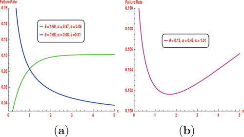
Some possible hrf and pdf shapes for the NKwE distribution are shown in Figures 1(a,b) and Figure 2(a,b). These figures illustrate that the NKwE distribution PDF can be symmetric, reversed-J shaped and right-skewed. The plots of HRF are sowing some flexible shapes, decreasing, upside-down bathtub-shaped, and reversed bathtub-shaped, which quantifies the lifetime distribution features, and it is used to understand the instantaneous rate of event occurrences over time, crucial in fields like survival analysis and reliability engineering.

Figure 1. Different graphical representations for pdf of the NKwE distribution.

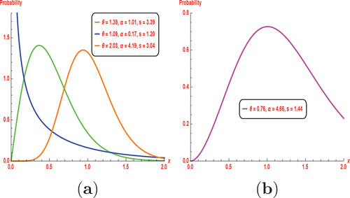
Figure 2. Different graphical representation for hrf of the NKwE distribution.

For the reason to express the qf of the NKwE distribution, the $p^{th}$ qf of the exponential distribution is received as $w_p=-\frac{1}{\theta }log(1-p)$. Thus, the $p^{th}$ qf denoted as $w_p$ of the NKwE distribution using Equation (7)(7) $w_p=G^{-1}\left[\left\{\left(\left({\left\{1-{(1-p)}^{1/s}\right\}}^{1/\alpha }-1\right)e^{-1}\right)+1\right\},\varpi \right],p\in (0,1).$(7) is obtained as

(10) $w_p=-\frac{1}{\theta }log\left\{1-\left[\left\{\left({\left(1-{\left(1-p\right)}^{1/s}\right)}^{1/\alpha }-1\right)e^{-1}\right\}+1\right]\right\}.$(10)

For the current study, median is taken as a quality parameter. Thus, to obtain median of the NkwE distribution can be obtained by replacing $p=0.5$ in Equation (10)(10) $w_p=-\frac{1}{\theta }log\left\{1-\left[\left\{\left({\left(1-{\left(1-p\right)}^{1/s}\right)}^{1/\alpha }-1\right)e^{-1}\right\}+1\right]\right\}.$(10) and is written as:

(11) $w_p=-\frac{1}{\theta }log\left\{1-\left[\left\{\left({\left(1-{\left(0.5\right)}^{1/s}\right)}^{1/\alpha }-1\right)e^{-1}\right\}+1\right]\right\}.$(11)

3. Description of GASP under the NKwE distribution

The layout parameter of a GASP is actually received within the scenario of the NKwE distribution. The procedures for bringing the organization reputation plan into action and acquiring architectural parameters were taken from Gupta (1962) and as follows:

• Creating a series of groups $g$ and giving each one $r$ objects. As a result, the lot sample size is $n=g\times r$.

• Choosing $c$ as the approval number for every group at time $w_0$.

• Carrying out the experiment for each of the $g$ groups at the same time and keeping track of how many attempts each group made failed.

• Accepting the outcome if there are no more than $c$ failures overall.

• If any group fails more than $c$ times, then the experiment is over and the lot will be discarded.

For a given $r$, the suggested GASP is specified by means of two parameters $(g,c)$. From Equation (8)(8) $F_{NKwE}\left(w\right)=1-{\left[1-{\left\{1-e^{-\theta w}{e}^{1-e^{-\theta w}}\right\}}^{\alpha }\right]}^s,$(8) , the cdf of the NKwE distribution is seen to be dependent on $t$, $\alpha$ and $s$, and the median life of the NKwE distribution is presented in Equation (10)(10) $w_p=-\frac{1}{\theta }log\left\{1-\left[\left\{\left({\left(1-{\left(1-p\right)}^{1/s}\right)}^{1/\alpha }-1\right)e^{-1}\right\}+1\right]\right\}.$(10) . It is proper to decide the termination time $w_0$ as $w_0=a_1{v}_0$, where $a_1$ denotes a positive regular and $v_0$ refers to the desired existence. For instance, if $a_1=0.5$, the test length is half that of the desired life, or if $a_1=3$, the test length is three times that of the required lifestyles. The probability of approving lots in this situation is

(12) $P_{a\left(p\right)}={\left[\sum _{j=0}^c\left(\begin{array}{c}r\\ j\end{array}\right)p^j{\left(1-p\right)}^{r-j}\right]}^g,$(12)

where “p” denotes the opportunity that an item in a set fails earlier than $t_0$, and the chance of failure is derived with the aid of putting Equation (10)(10) $w_p=-\frac{1}{\theta }log\left\{1-\left[\left\{\left({\left(1-{\left(1-p\right)}^{1/s}\right)}^{1/\alpha }-1\right)e^{-1}\right\}+1\right]\right\}.$(10) in (8). Based on Equation (10)(10) $w_p=-\frac{1}{\theta }log\left\{1-\left[\left\{\left({\left(1-{\left(1-p\right)}^{1/s}\right)}^{1/\alpha }-1\right)e^{-1}\right\}+1\right]\right\}.$(10) , we set

$v=-\frac{1}{\theta }log\left\{1-\left[\left\{\left({\left(1-{\left(1-p\right)}^{1/s}\right)}^{1/\alpha }-1\right)e^{-1}\right\}+1\right]\right\},$

Let,

$\phi =log\left\{1-\left[\left\{\left({\left(1-{\left(1-p\right)}^{1/s}\right)}^{1/\alpha }-1\right)e^{-1}\right\}+1\right]\right\}.$

Now, substituting $\theta =-\phi /v$ and $w=a_1{v}_0$ in Equation (8)(8) $F_{NKwE}\left(w\right)=1-{\left[1-{\left\{1-e^{-\theta w}{e}^{1-e^{-\theta w}}\right\}}^{\alpha }\right]}^s,$(8) , the failure probability is given by

$p=1-{\left\{1-{\left[1-e^{-\theta w}{e}^{\left(1-e^{-\theta w}\right)}\right]}^{\alpha }\right\}}^s,$

which can be expressed as

$p=1-{\left\{1-{\left[1-e^{\phi a_1{\left(v/v_0\right)}^{-1}}{e}^{\left(1-e^{\phi a_1{\left(v/v_0\right)}^{-1}}\right)}\right]}^{\alpha }\right\}}^s.$

When $a_1$ and $r_2=v/v_0$ are specific then it is possible to determine p for given $\alpha$ and $s$. A product’s agreeable stage may be expressed using the proportion of implied lifespan to the desired lifespan of a product as $v/v_0$. The only thing left to do is challenge the ensuring constraints while minimizing the $g$ and $c$ as min$\{g,c:(g,r,c)\}$, by considering the hypothesis as: $H_o:v=r_2\times v_0$ vs $H_1:v=r_1\times v_0$. The optimizing constraints are discussed below

(13) $P_{a\left(p_1|\frac{v}{v_0}=r_1\right)}={\left[\sum _{j=0}^c\left(\begin{array}{c}r\\ j\end{array}\right)p_1^j{\left(1-p_1\right)}^{r-j}\right]}^g\le \eta$(13)

and

(14) $P_{a\left(p_2|\frac{v}{v_0}=r_2\right)}={\left[\sum _{j=0}^c\left(\begin{array}{c}r\\ j\end{array}\right)p_2^j{\left(1-p_2\right)}^{r-j}\right]}^g\ge 1-{\alpha }_1,$(14)

where $r_1$ and $r_2$ denote the way ratio on the purchaser’s chance and at the producer’s hazard, respectively. The failing probabilities which can be utilised in the Equations (13)(13) $P_{a\left(p_1|\frac{v}{v_0}=r_1\right)}={\left[\sum _{j=0}^c\left(\begin{array}{c}r\\ j\end{array}\right)p_1^j{\left(1-p_1\right)}^{r-j}\right]}^g\le \eta$(13) and (14(14) $P_{a\left(p_2|\frac{v}{v_0}=r_2\right)}={\left[\sum _{j=0}^c\left(\begin{array}{c}r\\ j\end{array}\right)p_2^j{\left(1-p_2\right)}^{r-j}\right]}^g\ge 1-{\alpha }_1,$(14) ) are expressed as

(15) $p_1=1-{\left\{1-{\left[1-e^{\phi a_1}{e}^{\left(1-e^{\phi a_1}\right)}\right]}^{\alpha }\right\}}^s$(15)

and

(16) $p_2=1-{\left\{1-{\left[1-e^{\phi a_1{\left(v/v_0\right)}^{-1}}{e}^{\left(1-e^{\phi a_1{\left(v/v_0\right)}^{-1}}\right)}\right]}^{\alpha }\right\}}^s.$(16)

Both the above Equations (15)(15) $p_1=1-{\left\{1-{\left[1-e^{\phi a_1}{e}^{\left(1-e^{\phi a_1}\right)}\right]}^{\alpha }\right\}}^s$(15) and (16(16) $p_2=1-{\left\{1-{\left[1-e^{\phi a_1{\left(v/v_0\right)}^{-1}}{e}^{\left(1-e^{\phi a_1{\left(v/v_0\right)}^{-1}}\right)}\right]}^{\alpha }\right\}}^s.$(16) ) are extracted from Equation (14)(14) $P_{a\left(p_2|\frac{v}{v_0}=r_2\right)}={\left[\sum _{j=0}^c\left(\begin{array}{c}r\\ j\end{array}\right)p_2^j{\left(1-p_2\right)}^{r-j}\right]}^g\ge 1-{\alpha }_1,$(14) .

4. Description of GASP with example

The utilization of a sampling technique is claimed to be beneficial in terms of saving both time and money. Various sampling methods involve conducting specific quality control tests to determine whether a batch should be approved or rejected. This particular section revolves around an illustration of a GASP (grouped age sampling plan) that operates on the assumption that the distribution of an item’s lifespan follows an NKwE model, with the shape parameters $\alpha$ and $s$ known, and utilizes the cumulative distribution function described in Equation (8)(8) $F_{NKwE}\left(w\right)=1-{\left[1-{\left\{1-e^{-\theta w}{e}^{1-e^{-\theta w}}\right\}}^{\alpha }\right]}^s,$(8) . In this GASP scenario, a random sample of size n is chosen, distributed and subjected to life screening for $r$ item within each group over a predetermined time period. However, Tables 1 and 2 show the layout parameters for GASP with distinctive values of s $(1.02$ and $2.0)$. Taken into account that $r$ has values (5 and 10). Additionally, it has been also shown that reducing customer risk broadens the variety of enterprises. Moreover, as $r_2$ rises, the range of companies shrinks fast. Beyond a certain factor, the number of companies and approval rates stay consistent, and the likelihood of approving a massive quantity gradually starts to decline. To represent an effect of $a_1$ is also proven inside the table. On the life take a look at, for example, $\eta =0.25$, $a_1=0.5$, $r_2=6$, $s=1.02$, and $r=5$, for eight groups 40 $(8\times 5)$ units, are required. Furthermore, for $r=10$, the life test calls for best agencies, i.e., $2\times 5=10$ units. As an end result, 10 organizations would be ideal in this scenario. Table 2 has a value of 2.0. Increasing the form parameter price effects in a reduced group length for the connected plan, consistent with the said data. When the real median lifestyles grow, the variety of corporations drops and the OC values $P(a)$ growth for the investigated GASP when using the NKwE distribution and median lifetime as the first-class criterion. It is supplied in Table 2 for numerous parametric values ($s=1.02$, $\eta =0.25$, $r=5$ and $a_1=0.5$). An example from Smith et al. (2023) is taken into consideration while displaying Table 3 to pass test the effects displayed in Tables 1 and 2.

Table 1. GASP displaying minimal $g$ and $c$ for $\alpha =0.5$ and $s=1.02$

		r = 5						r = 10
		a1 = 0.5			a1 = 1			a1 = 0.5			a1 = 1
η	r2	g	c	p(a)	g	c	p(a)	g	c	p(a)	g	c	p(a)
	2	-	-	-	-	-	-	-	-	-	-	-	-
0.25	4	4	2	0.9539	3	3	0.9733	2	3	0.9627	1	4	0.9555
	6	4	2	0.9849	1	2	0.9746	1	2	0.9657	1	3	0.9528
	8	4	2	0.9933	1	2	0.9883	1	2	0.9837	1	3	0.9812
	2	-	-	-	-	-	-	-	-	-	-	-	-
0.1	4	26	3	0.9817	4	3	0.9645	6	4	0.9839	1	4	0.9555
	6	7	2	0.9737	4	3	0.9917	3	3	0.9861	1	3	0.9528
	8	7	2	0.9883	2	2	0.9767	2	2	0.9677	1	3	0.9812
	2	-	-	-	-	-	-	-	-	-	-	-	-
0.05	4	34	3	0.9761	23	4	0.9893	7	4	0.9812	3	5	0.9719
	6	8	2	0.9700	6	3	0.9876	4	3	0.9815	1	3	0.9528
	8	8	2	0.9866	2	2	0.9767	2	2	0.9677	1	3	0.9812
	2	-	-	-	-	-	-	-	-	-	-	-	-
0.01	4	52	3	0.9637	35	4	0.9837	11	4	0.9706	4	5	0.9628
	6	13	2	0.9517	8	3	0.9835	5	3	0.9769	2	4	0.9818
	8	13	2	0.9784	4	2	0.9539	3	2	0.9520	2	3	0.9627

Note: A large sample length in needed cells contains hyphens (-).

Table 2. GASP displaying minimal $g$ and $c$ for $\alpha =0.8$ and $s=2.0$

	r = 5								r = 10
	a1 = 0.5					a1 = 1			a1 = 0.5			a1 = 1
η	r2		g	c	p(a)	g	c	p(a)	g	c	p(a)	g	c	p(a)
	2		18	3	0.9565	6	4	0.9508	4	4	0.9565	-	-	-
0.25	4		5	2	0.9924	1	2	0.9714	1	2	0.9851	1	4	0.9889
	6		2	1	0.9838	1	2	0.9946	1	1	0.9668	1	2	0.9532
	8		2	1	0.9932	1	1	0.9729	1	1	0.9856	1	2	0.9851
	2		274	4	0.9765	-	-	-	16	5	0.9748	-	-	-
0.1	4		7	2	0.9893	3	3	0.9926	2	2	0.9704	1	4	0.9889
	6		3	1	0.9758	2	2	0.9893	1	1	0.9668	1	2	0.9532
	8		3	1	0.9898	1	1	0.9729	2	1	0.9856	1	2	0.9851
	2		357	4	0.9695	-	-	-	20	5	0.9686	-	-	-
0.05	4		9	2	0.9863	4	3	0.9902	2	2	0.9704	1	4	0.9889
	6		3	1	0.9758	2	2	0.9893	2	2	0.9948	1	2	0.9532
	8		3	1	0.9898	1	1	0.9729	2	1	0.9714	1	2	0.9851
	2		584	4	0.9536	-	-	-	31	5	0.9517	-	-	-
0.01	4		14	2	0.9788	5	3	0.9877	3	2	0.9559	2	4	0.9780
	6		5	1	0.9599	3	2	0.9839	3	2	0.9922	1	2	0.9532
	8		5	1	0.9831	3	2	0.9954	2	1	0.9714	1	2	0.9851

Note: A large sample length in needed cells contains hyphens (-).

Table 3. $s=1.02$$\eta =0.25$ $r=5$ and $a_1=0.5$

$v$/$v_0$=$r_2$	4	6	8
$g$	4	4	4
$c$	2	2	2
$p(a)$	0.9539	0.9849	0.9933

Assuming that the intended lifespan for motor of clock positioned on the NKwE distribution with shape parameter $s=1.02$ is 4000 cycles. When the actual median lifetime is 4000 cycles as opposed to the actual prescribed lives of 8000 cycles, the producer confronts a 5% risk while the customer suffers a 25% risk. An analyst will now do a 2000-cycle test with 10 units within every group to check if the indicated lifespan motor of clock is larger than their intended lifespan. For this scenario, we have $s=1.02$, $v_0$ = 4000 cycles, $a_1=$0, $r=5$, $\eta =$0.25, $r_1=1$, producer’s risk = 0.05 with $r_2=2$. Moreover, in Table 2, we have $g=64$ and $c=7$. It means that 640 $(64\times 10)$ units have to be drawn, with 5 devices being allocated to each of the 64 groups. If no greater than 7 units expire in all of those companies before a thousand cycles, the implied lifestyles for the motor of clock can be statistically guaranteed to be extra than the prescribed lifestyles. If a first-rate manipulate investigator wants to test the idea that the motor of clock has a lifespan of $8000$ cycles but a real average existence of four times that the investigator can test $64$ companies of five different items. If no more than three items expire in $2000$ cycles, the investigator will conclude that the lifespan is greater than $8000$ cycles with 95% of accuracy because $a_1=0.5$ and the median lifespan is $2000$ cycles. Therefore, the lot below research needs to be familiar.

Figure 3 demonstrates that how the $g$ and $c$ values tend to decrease as the actual median lifetime increases while the operating characteristic (OC) values tend to steadily increase. Therefore, the lot under consideration will be accepted within certain periods. Accepting the lot at $r=10$ would be preferable in this instance for optimizing time and money, since fewer groups would be assessed than $r=5$ while by taking, $(a)$ $s=1.25$ $\beta =0.1$ $r=5$ $a_1=0.5$, $(b)$ $s=1.25$ $\beta =0.1$ $r=5$ $a_1=0.5$, $(c)$ $s=1.5$ $\beta =0.25$ $r=10$ $a_1=0.5$, $(d)$ $s=1.5$ $\beta =0.25$ $r=10$ $a_1=0.5$ respectively.

Figure 3. Tables 1 and 2 [1] and [2] are used as the sources of some parametric values for the graphical representation of g and OC.

5. Application

5.1. Data set I

The first data set represents average daily wind speeds (in meter/second) in November 2007 at Elanora Heights, a northeastern suburb of Sydney, Australia, described by Maiti and Kayal (2020). This is how the data set can be increased (0.5833, 0.6667, 0.6944, 0.7222, 0.7500, 0.7778, 0.8056, 0.8056, 0.8611, 0.8889, 0.9167, 1.0000, 1.0278, 1.0278,1.1111,1.1111, 1.1111, 1.1667, 1.1667,1.1944, 1.2778, 1.2778, 1.3056, 1.3333, 1.3333, 1.3611, 1.4444, 2.1111,2.1389,2.7778).

The p-value (PV), standard error (SE), Kolmogorov–Smirnov (KS), and maximum likelihood estimate (MLEs) of the NKwE distribution are shown in Table 4.

Table 4. The MLEs (SE), KS, and p-value for data set I

Parameter	MLEs (SE)	KS	PV
$\hat{\theta }$	84.7012 (49.9827)	0.1114	0.8499
$\hat{\alpha }$	0.2927 (0.0960)
$\hat{s}$	0.3132 (0.2748)

The histogram of the records with the estimated pdf, estimated cdf, Probability-Probability (P-P) plot, Quantiles-Qunatiles (Q-Q) plot, TTT, and envisioned hrf is shown in Figure 4. Figure 4 indicates that the NKwE model has a good modelled for the survival record set. According to estimated parametric values, the planned parameters are likewise determined and are displayed in Table 5. The results of the anticipated parameters in Table 5 are shown to be consistent with the values in Tables 1 and 2.

Figure 4. (a) Estimate the density, (b) estimate the cdf, (c) P-P, (d) Q-Q, (e) TTT, and (f) estimate the hrf.

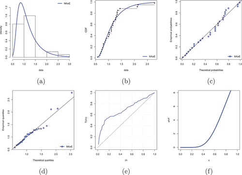
Table 5. GASP under NKwE model, $\hat{\alpha }$ = 0.2927 and $\hat{s}$ = 0.3132, displaying minimal $g$ and $c$

		r = 5						r = 10
		a1 = 0.5			a1 = 1			a1 = 0.5			a1 = 1
η	r2	g	c	p(a)	g	c	p(a)	g	c	p(a)	g	c	p(a)
	2	-	-	-	-	-	-	-	-	-	-	-	-
0.25	4	34	3	0.9674	6	3	0.9625	7	4	0.9731	3	5	0.9824
	6	7	2	0.9540	6	3	0.9873	3	3	0.9718	1	3	0.9520
	8	7	2	0.9734	2	2	0.9708	3	3	0.9859	1	3	0.9752
	2	-	-	-	-	-	-	-	-	-	-	-	-
0.1	4	658	4	0.9829	62	4	0.9818	11	4	0.9581	5	5	0.9709
	6	57	3	0.9814	10	3	0.9790	5	3	0.9535	3	4	0.9722
	8	11	2	0.9585	10	3	0.9903	5	3	0.9766	2	1	0.9511
	2	-	-	-	-	-	-	-	-	-	-	-	-
0.05	4	856	4	0.9779	81	4	0.9762	44	5	0.9813	6	5	0.9652
	6	74	3	0.9759	13	3	0.9728	6	3	0.9720	3	4	0.9722
	8	74	3	0.9887	13	3	0.9874	15	4	0.9835	2	3	0.9511
	2	-	-	-	-	-	-	-	-	-	-	-	-
0.01	4	-	-	-	124	4	0.9639	68	5	0.9712	-	-	-
	6	113	3	0.9635	20	3	0.9584	22	4	0.9760	5	4	0.9541
	8	113	3	0.9828	20	3	0.9807	9	3	0.9582	5	4	0.9807

Note: A large sample length in needed cells contains hyphens (-).

5.2. Data set II

The second piece of data came from Rasay et al. (2020) which records 23 failure rates for deep-grove ball bearings (in millions of revolution). The data set II is given as (17.88, 28.92, 33.00, 41.52, 42.12, 45.60, 48.40, 51.84, 51.96, 54.12, 55.56, 67.80, 68.64, 68.64, 68.88, 84.12, 93.12, 98.64, 105.12, 105.84, 27.92, 128.04, 173.40).

The p-value (PV), standard error (SE), Kolmogorov–Smirnov (KS), and maximum likelihood estimate (MLEs) of the NKwE distribution are shown in Table 6.

Table 6. The MLEs (SE), KS, and p-value for data set II

Parameter	MLEs (SE)	KS	PV
$\hat{\theta }$	0.0071 (0.0015)	0.1377	0.7754
$\hat{\alpha }$	1.1721 (0.2574)
$\hat{s}$	12.1036 (3.9690)

The histogram of the records with the estimated pdf, estimated cdf, Probability-Probability (P-P) plot, Quantiles-Qunatiles (Q-Q) plot, TTT, and envisioned hrf is shown in Figure 5.

Figure 5. (a) Estimate the density, (b) estimate the cdf, (c) P-P, (d) Q-Q, (e) TTT, and (f) estimate the hrf.

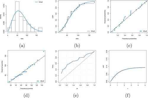
Figure 5 indicates that the NKwE model has a good modelled for the survival record set. Thus, the NKwE model gives a reasonable suit of the statistics. The plan parameters are calculated using fitted parametric values and are shown in Table 7. It can be observed that the performance of the planned parameters in Table 7 is consistent with the values in Tables 1 and 2.

Table 7. GASP under NKwE model, $\hat{\alpha }$ = 2.5047 and $\hat{s}$ = 12.7570, displaying minimal $\mathit{g}$ and $\mathit{c}$

		r = 5						r = 10
		a1 = 0.5			a1 = 1			a1 = 0.5			a1 = 1
η	r2	g	c	p(a)	g	c	p(a)	g	c	p(a)	g	c	p(a)
	2	3	3	0.9789	-	-	-	-	-	-	-	-	-
0.25	4	1	1	0.9805	1	3	0.9929	2	2	0.9815	1	4	0.9653
	6	1	1	0.9967	1	2	0.9942	1	1	0.9860	1	2	0.9501
	8	1	0	0.9529	1	1	0.9805	1	1	0.9961	1	2	0.9907
	2	5	3	0.9650	-	-	-	-	-	-	-	-	-
0.1	4	1	1	0.9805	1	3	0.9929	2	2	0.9815	1	4	0.9653
	6	1	1	0.9967	1	2	0.9942	1	1	0.9860	1	2	0.9501
	8	1	0	0.9529	1	1	0.9805	1	1	0.9961	1	2	0.9907
	2	6	3	0.9582	-	-	-	-	-	-	-	-	-
0.05	4	2	1	0.9613	1	3	0.9929	3	2	0.9723	-	-	-
	6	2	1	0.9934	1	2	0.9942	2	1	0.9723	1	2	0.9501
	8	1	0	0.9529	1	1	0.9805	2	1	0.9921	1	2	0.9907
	2	41	4	0.986	-	-	-	-	-	-	-	-	-
0.01	4	2	1	0.9613	1	3	0.9929	4	2	0.9632	-	-	-
	6	2	1	0.9934	1	2	0.9942	2	1	0.9723	1	2	0.9501
	8	1	0	0.9529	1	1	0.9805	2	1	0.9921	1	2	0.9907

Note: A large sample length in needed cells contains hyphens (-).

The descriptive analysis of two data sets is shown in Table 8, and all values were calculated by using the R-programming language and graphically presented in Figure 6 which includes the sample size $(n)$, maximum claim $(z_n)$, minimum claim $(z_0)$, lower quartile $(Q_1)$, upper quartile $(Q_3)$, mean $(\bar{z})$, median $(\tilde{z})$, standard deviation $(\sigma )$, measure of skewness $(S_k)$, and kurtosis $(k)$, respectively.

Figure 6. Plots of descriptive analysis for (a) data set I and (b) data set II.

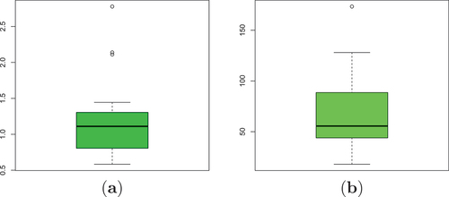
Table 8. Descriptive analysis of data sets

Data set	n	z0	Q1	$\tilde{\mathbf{z}}$	$\bar{\mathbf{z}}$	σ	Q3	zn	SK	K
I	30	0.58	0.81	1.11	1.15	0.475	1.29	2.77	1.741	6.281
II	23	17.88	43.86	55.56	67.87	36.524	88.62	173.40	1.137	4.1808

Table 9 is showing the true median lifetimes, sample sizes, $g$, $c$, and OC values of two data sets. Considering data set I with $\eta =0.01$, $r=5$, $a_1=0.5$, $\hat{\alpha }$ = 1.1253 and $\hat{s}$ = 3.4506 when $g$ and $c$ decrease and probability increase, the lot will be accepted. Similarly, considering data set II with $\eta =0.01$, $r=10$, $a_1=0.5$, $\hat{\alpha }$ = 2.5047 and $\hat{s}$ = 12.7570 when $g$ and $c$ decrease and probability increase, the lot will be accepted. Here, it is cleared that for data sets I and II, the lesser groups are to be tested, and hence it will optimize cost and time.

Table 9. True median lifetimes, sample sizes, $g$, $c$, and OC values of the two data sets

	Data set I				Data set II
$v$/$v_0$=$r_2$	2	4	6	8	$v$/$v_0$=$r_2$	2	4	6	8
$n$	430	30	30	30	$n$	-	40	20	20
$g$	86	6	6	6	$g$	-	4	2	2
$c$	3	1	1	1	$c$	-	2	1	1
$p(a)$	0.9659	0.9713	0.9949	0.9986	$p(a)$	-	0.9632	0.9723	0.9921

6. Comparative study of GASP versus OSP

A procedure characterized as batch judgement uses ASPs to decide whether the coming or leaving batches should be admitted or denied according to a predetermined quality. The sample size and duration of investigation are the two factors that experienced professionals should consider most carefully, and both should be optimized. Although the OSP can help with this optimization, in such a case, only a single item will be evaluated at a time. In contrast, a GASP may also accomplish the optimal expense and hassle when several items can be evaluated by grouping them together. Table 10 shows the sample sizes of the GASP and OSP when $\eta =0.25$ and $a_1=0.5$ for the two datasets. It is evident from Table 10 that GASP is superior to OSP as minimum items are to be tested at once, which results in optimized time and cost.

Table 10. Sample sizes of GASP and OSP

		Data set I		Data set II
		a1= 0.5		a1= 0.5
η	r2	GASP	OSP	GASP	OSP
	2	33	36	15	17
0.25	4	11	14	5	7
	6	12	15	5	7
	8	6	9	6	8

7. Conclusion

This study focuses on a GASP that assumes the lifespan of a product will follow the NKwE distribution. The study emphasizes a few critical plan parameters, specifically the number of groups $g$ and acceptance number $c$, which are determined by balancing the risks of producers and consumers. The proposed plan aims to maintain a specific quality level by setting a limit on the number of defective items that can be present in a batch. As the percentile ratio (the ratio of the true average life to the stipulated life) increases in the proposed plan, the number of groups $g$ and the acceptance number $c$ tend to decrease, while the operational characteristics (OC) values tend to increase. The study concludes that the proposed plan is effective in ensuring that a specific level of quality is maintained while also minimizing the risks for both the producer and the consumer. By balancing the risks, the plan helps prevent the acceptance of defective items while avoiding the rejection of good products. Overall, this study contributes to the development of the GASP methodology for products with a lifespan that follows NKwE distribution. The proposed plan can be useful for manufacturers and consumers in various industries as it provides a way to ensure product quality while minimizing risk. The applicability and effectiveness of GASP may vary depending on the specific industry, product characteristics, and quality requirements. Engineers should carefully assess the suitability of GASP for their particular situations and consult relevant standards and guidelines to ensure its proper implementation.

Disclosure statement

No potential conflict of interest was reported by the author(s).

Data availability statement

The data presented in this study are available on request from the corresponding author.

Additional information

Funding

No funding was obtained for this study.

References

- Alexander, C., Cordeiro, G. M., Ortega, E. M. M., & Sarabia, J. M. (2012). Generalized beta-generated distributions. Computational Statistics & Data Analysis, 56(6), 1880–18. https://doi.org/10.1016/j.csda.2011.11.015
- Almarashi, A. M., Khan, K., Chesneau, C., & Jamal, F. (2021). Group acceptance sampling plan using Marshall Olkin Kumaraswamy exponential (MOKw-E) distribution. Processes, 9(6), 1066. https://doi.org/10.3390/pr9061066
- Ameeq, M., Tahir, M. H., Hassan, M. M., Jamal, F., Shafiq, S., & Mendy, J. T. (2023). A group acceptance sampling plan truncated life test for alpha power transformation inverted perks distribution based on quality control reliability. Cogent Engineering, 10(1), 2224137. https://doi.org/10.1080/23311916.2023.2224137
- Aslam, M., Balamurali, S., Jun, C. H., & Ahmad, M. (2013). Optimal design of skip lot group acceptance sampling plans for the Weibull distribution and the generalized exponential distribution. Quality Engineering, 25(3), 237–246. https://doi.org/10.1080/08982112.2013.769053
- Aslam, M., & Jun, C. H. (2009a). A group acceptance sampling plan for truncated life test having Weibull distribution. Journal of Applied Statistics, 36(9), 1021–1027. https://doi.org/10.1080/02664760802566788
- Aslam, M., Jun, C.-H., & Ahmad, M. (2009). A group acceptance sampling plan based on truncated life test for gamma distributed items. Pakistan Journal of Statistics, 25(3), 333–340.
- Aslam, M., & Jun, C. H. (2009b). A group acceptance sampling plans for truncated life tests based on the inverse Rayleigh and log-logistic distributions. Pakistan Journal of Statistics, 25(2). https://doi.org/10.1515/eqc.2010.008
- Aslam, M., Kundu, D., & Ahmad, M. (2010). Time truncated acceptance sampling plans for generalized exponential distribution. Journal of Applied Statistics, 37(4), 555–566. https://doi.org/10.1080/02664760902769787
- Attali, C., Huez, J. F., Valette, T., & Lehr-Drylewicz, A. M. (2013). Les grandes familles de situations cliniques. Exercer, 24(108), 165–169.
- Azzalini, A. (1985). A class of distributions which includes the normal ones. Scandinavian Journal of Statistics, 171–178.
- Baklizi, A. (2003). Acceptance sampling based on truncated life tests in the pareto distribution of the second kind. Advances and Applications in Statistics, 3(1), 33–48.
- Balakrishnan, N., Leiva, V., & Lopez, J. (2007). Acceptance sampling plans from truncated life tests based on the generalized Birnbaum-Saunders distribution. Communications in Statistics-Simulation and Computation, 36(3), 643–656. https://doi.org/10.1080/03610910701207819
- Bourguignon, M., Silva, R. B., & Cordeiro, G. M. (2014). The Weibull-G family of probability distributions. Journal of Data Science: JDS, 12(1), 53–68. https://doi.org/10.6339/JDS.201401_12(1).0004
- Chang, J. F. (2016). Business process management systems: Strategy and implementation. CRC Press. https://doi.org/10.1201/9781420031362
- Cordeiro, G. M., & de Castro, M. (2011). A new family of generalized distributions. Journal of Statistical Computation and Simulation, 81(7), 883–898. https://doi.org/10.1080/00949650903530745
- Duncan, A. J. (1986). Quality control and industrial Statistics (5th. ed.). Richard D Irvin.
- El-Morshedy, M., Tahir, M. H., Hussain, M. A., Al-Bossly, A., & Eliwa, M. S. (2022). A New flexible univariate and bivariate family of distributions for unit interval (0, 1). Symmetry, 14(5), 1040. https://doi.org/10.3390/sym14051040
- Epstein, B. (1954). Truncated life tests in the exponential case. Annals of Mathematical Statistics, 25(3), 555–564. https://doi.org/10.1214/aoms/1177728723
- Eugene, N., Lee, C., & Famoye, F. (2002). Beta-normal distribution and its applications. Communications in Statistics: Theory and Methods, 31(4), 497–512. https://doi.org/10.1081/STA-120003130
- Gleaton, J. U., & Lynch, J. D. (2006). Properties of generalized log-logistic families of lifetime distributions. Journal of Probability and Statistical Science, 4, 51–64.
- Goode, H. P., & KAO, J. H. (1961). An adaptation of the MIL-STD-105B plans to reliability and life testing applications. CORNELL UNIV ITHACA NY.
- Gupta, S. S. (1962). Life test sampling plans for normal and lognormal distributions. Technometrics, 4(2), 151–175. https://doi.org/10.1080/00401706.1962.10490002
- Gupta, R. C., Gupta, P. L., & Gupta, R. D. (1998). Modeling failure time data by Lehman alternatives. Communications in Statistics: Theory and Methods, 27(4), 887–904. https://doi.org/10.1080/03610929808832134
- Jun, C. H., Balamurali, S., & Lee, S. H. (2006). Variables sampling plans for Weibull distributed lifetimes under sudden death testing. IEEE Transactions on Reliability, 55(1), 53–58. https://doi.org/10.1109/TR.2005.863802
- Kantam, R. R. L., Rosaiah, K., & Rao, G. S. (2001). Acceptance sampling based on life tests: Log-logistic models. Journal of Applied Statistics, 28(1), 121–128. https://doi.org/10.1080/02664760120011644
- Kumaraswamy, P. (1980). Generalized probability density function for double bounded random processes. Journal of Hydrology, 46(1–2), 79–88. https://doi.org/10.1016/0022-1694(80)90036-0
- Maiti, K., & Kayal, S. (2020). Estimating reliability characteristics of the log logistic distribution under progressive censoring with two applications. Data Science, 10(1), 1–40. https://doi.org/10.1007/s40745-020-00292-y
- Marshall, A. W., & Olkin, I. (1997). A new method for adding parameters to a family of distributions with application to the exponential and Weibull families. Biometrika, 84(3), 641–652. https://doi.org/10.1093/biomet/84.3.641
- Muneeb Hassan, M., Ameeq, M., Jamal, F., Tahir, M. H., & Mendy, J. T. (2023). Prevalence of COVID-19 among patients with chronic obstructive pulmonary disease and tuberculosis. Annals of Medicine, 55(1), 285–291. https://doi.org/10.1080/07853890.2022.2160491
- Naz, S., Al-Essa, L. A., Bakouch, H. S., & Chesneau, C. (2023). A transmuted modified power-generated family of distributions with practice on submodels in insurance and reliability. Symmetry, 15(7), 1458. https://doi.org/10.3390/sym15071458
- Rao, G. S. (2009a). A group acceptance sampling plans based on truncated life tests for Marshall-Olkin extended Lomax distribution. Electronic Journal of Applied Statistical Analysis, 3(1), 18–27.
- Rao, G. S. (2009b). A group acceptance sampling plans for lifetimes following a generalized exponential distribution. Economic Quality Control, 24(1). https://doi.org/10.1515/EQC.2009.75
- Rasay, H., Naderkhani, F. G., & M, A. (2020). Designing variable sampling plans based on lifetime performance index under failure censoring reliability tests. Quality Engineering, 32(3), 354–370. https://doi.org/10.1080/08982112.2020.1754426
- Rezaei, S., Sadr, B. B., Alizadeh, M., & Nadarajah, S. (2017). Topp–Leone generated family of distributions: Properties and applications. Statistical Theory Methods, 46(6), 2893–2909. https://doi.org/10.1080/03610926.2015.1053935
- Rosaiah, K., Kantam, R. R. L., & Rao, B. S. (2009). Reliability test plan for half logistic distribution. Calcutta Statistical Association Bulletin, 61(1–4), 183–196. https://doi.org/10.1177/0008068320090110
- Rubmann, M., Lorenz, M., Gerbert, P., Waldner, M., Justus, J., Engel, P., & Harnisch, M. (2015). Industry 4.0: The future of productivity and growth in manufacturing industries. Boston Consulting Group, 9(1), 54–89.
- Smith, O. M., Davis, K. L., Pizza, R. B., Waterman, R., Dobson, K. C., Foster, B., & Davis, C. L. (2023). Peer review perpetuates barriers for historically excluded groups. Nature Ecology Evolution, 7(4), 512–523. https://doi.org/10.1038/s41559-023-01999-w
- Tahir, M. H., Cordeiro, G. M., Alizadeh, M., Mansoor, M., Zubair, M., & Hamedani, G. G. (2015). The odd generalized exponential family of distributions with applications. Journal of Statistical Distributions and Applications, 2(1), 2. https://doi.org/10.1186/s40488-014-0024-2
- Vlcek, B. L., Hendricks, R. C., & Zaretsky, E. V. (2004). Monte Carlo simulation of sudden death bearing testing. Tribology Transactions, 47(2), 188–199. https://doi.org/10.1080/05698190490431867