A new Bell-exponential model: Properties and applications

Abstract

In this paper, we propose a tractable Kumaraswamy Bell exponential (KwBE) distribution as a submodel of the Kumaraswamy Bell-G family of distributions. Several well-established properties are obtained for the KwBE distribution, such as the linear functional representation, $r$th moment, incomplete moment, moment generating function using Wright generalized hyper-geometric function, conditional moment and Réyni entropy. Based on the KwBE model, a group acceptance sampling plan (GASP) for the truncated life test is presented using median life as a quality index. Moreover, the essential design parameters are derived by defining the consumer risk and the test termination duration. The comparative study of GASP with ordinary sampling plan (OSP) is performed. A simulation study is performed to highlight the behavior of the estimates. On the inferential side, the associated parameters are estimated using a well-established maximum likelihood estimation method. The detailed model’s comparison analysis, graphical as well as numerical evidence to real-data applications, supports the theoretical work.

Keywords:

• acceptance sampling
• entropy
• estimation
• simulation
• statistical model
• quality parameter

1. Introduction with aims

Statistical models are essential in many social and scientific investigations. On the other side, quality control is an important statistical domain that is the collection of statistical tools responsible for ensuring and monitoring the product quantity and quality governed by the models. One of the most popular statistical quality control techniques is the acceptance sampling plan (ASP), which is used to evaluate and decide whether to accept or reject the chosen products based on a sample as well as to check the integrity of products. Generally, ASP is an optimization method to minimize the sample size or a particular cost function for destructive items, while considering a variety of constraints set forth by the supplier and client. The sentencing lot might be either raw materials, modules, or finalized commodities. A lot may be inspected either after fabrication or immediately before being shipped to the supplier. Consumers inspect merchandise once they have received it. Departing inspection is the phrase for a producer’s certification, whereas arriving inspection is the terminology for a customer’s assessment (Khan et al., 2022). Because of time and financial constraints, a $100\mathrm{\%}$ screening cannot be emphasised in the mass of statistical quality assurance trials (Algarni, 2022). Consequently, an ASP serves as a mid-route between $100\mathrm{\%}$ and $0\mathrm{\%}$ inspections (Aslam et al., 2011). An ASP is a helpful technique for testing delicate, pricey objects or when the possible legal obligations are higher. Acceptance sampling is a helpful technique for testing delicate, pricey objects or when the possible legal obligations are higher. A favorable lot could be discarded in an acceptance sample, or a defective lot might be approved, both of which are undesired outcomes. Retailer’s risks refer to the first scenario usually denoted as $\alpha$, in which a quality lot is refused, and customer’s risks refer to the second scenario usually denoted as $\beta$, in which a disastrous lot is approved (Khan et al., 2022). Furthermore, these ASPs are classified as variable, attributes, accelerated, progressively and group acceptance sampling plans. Nevertheless, the primary goal of these strategies is to protect both the manufacturer and the client while evaluating the sentenced lot using the least sample size. The group acceptance sampling plan (GASP) is the widely used sampling plan and is found superior to any other plan because it is subjected always to optimize cost and time of inspecting the quality of the lot by testing multiple items at once. One may get the optimum sample size along with test duration feasible with the use of a GASP. The underlying premise of the OSP entails that each trial will carry only a single item and hence always results in a hectic time-testing procedure with increased cost. Conversely, in reality, testers who can test many products at once are employed since doing so may cut down testing expenses and time. The result of integrating GASP with curtailed life testing is a GASP based on truncated life tests, which is premised on the presumption that the duration of a product matches a particular probability distribution. The attribute GASP for the truncated life test was developed by (Aslam & Jun, 2009a), who assumed that each lifespan of a product followed the Weibull distribution. The economic reliability GASP was developed by (Aslam et al., 2010) for the Pareto distribution of the second kind. The repetitive GASP for the Burr XII distribution was developed by (Aslam et al., 2013). The skip lot GASP was developed by (Aslam et al., 2013) for the Weibull distribution. For specific values of the producer and consumer risks, these sampling plans concurrently determine the frequency of the groups and acceptance numbers. A GASP for the truncated life test, when the lifetime of an item followed the log-logistic inverse Rayleigh distribution, was developed by (Aslam & Jun, 2009b). Several other researchers who developed a GASP are Reference (Aslam et al., 2011) developed GASP for the generalized exponential model (Rao, 2009), for the Marshall-Olkin extended Lomax model (Ameeq et al., 2023), for the alpha power transformation model (Naz et al., 2023), for the kumaraswamy exponential model (Almarashi et al., 2021), for the Marshall-Olkin Kumaraswami exponential model (Tsai & Wu, 2006), for the generalized Rayleigh model (Balakrishnan et al., 2007), for the Birnbaum-Saunders model (Fayomi et al., 2022), for the exponentiated Bell exponential model and (Algarni, 2022) for the compounded three-parameter Weibull model.

However, developing enlarged flexible statistical models has become a common practice (Muneeb Hassan et al., 2023; Tahir & Cordeiro, 2016; Tahir & Nadarajah, 2015). The ultimate objective of this entire exercise is to improve the convergent validity of the constructed model and the effective examination of skewness and tail aspects. These expanded models offer practitioners and applied researchers a better understanding of the pattern and evolution of complicated real-world phenomena, ultimately achieving better estimation and optimization (Hassan et al., 2023, 2023). Generalized classes (G-classes) and compounding are the two main considered generalization techniques that are frequently used and put into practice. Here, we mention a few but not limited, the readers are referred to Marshall-Olkin-G (Marshall & Olkin, 1997), exponentiated-G (Gupta et al., 1998), beta-G (Eugene et al., 2002), Transmuted modified power-G (Naz et al., 2023) and McDonald-G (Alexander et al., 2012). Based on the genesis of the Kw distribution, Cordeiro and de Castro (Cordeiro & de Castro, 2011) presented a highly effective family of generalized distributions, even with censored data. From an arbitrary baseline cumulative distribution function (CDF) $G(x)$ and corresponding probability density function (PDF) $g(x)$, the CDF $F^{\mathrm{K}\mathrm{w}\mathrm{G}}\left(x,a,b,\xi \right)$ and the PDF $f^{\mathrm{K}\mathrm{w}\mathrm{G}}\left(x,a,b,\xi \right)$, respectively, of the Kw-G family (Cordeiro & de Castro, 2011) are given by

(1) $F^{\mathrm{K}\mathrm{w}\mathrm{G}}\left(t,a,b,\xi \right)=1-{\left[1-G{\left(t\right)}^a\right]}^b$(1)

and

(2) $f^{\mathrm{K}\mathrm{w}\mathrm{G}}\left(t,a,b,\xi \right)=abg(t)G(t{)}^{a-1}{\left[1-G{(t)}^a\right]}^{b-1},$(2)

where $t,a,b>0,$ and the two parameters $a$ and $b$ that interact with the specific role of incorporating skewness and adjusting the tail weights. The Kw-G family has some similarities to the well-known beta-G family given by Eugene et al. (Eugene et al., 2002), the readers are referred to (Cordeiro & de Castro, 2011) for the larger extent of the interconnections and advantages of the Kw-G family over the Beta-G family.

An alternative to the commonly used Poisson distribution is a single parameter discrete Bell distribution given by (Castellares et al., 2018), which yields somewhat better fits even for over-dispersion data than the Poisson distribution. This distribution involves the features of well-known Bell numbers (Bell, 1934) and belongs to the exponential family. Exponentiated Bell-G family, an extended class of Bell distribution recently presented by Fayomi et al. (Fayomi et al., 2022), is an analog to exponentiated Poisson-G and demonstrates its usefulness and practical relevance. The genesis of the Bell distribution is used to construct the next family of distributions with the following CDF (Fayomi et al., 2022):

(3) $F^{\mathrm{B}\mathrm{G}}(t;\varpi )=\frac{1-exp\left(-e^{\varpi }\left[1-e^{-\varpi G(t)}\right]\right)}{1-exp(1-e^{\varpi })}.$(3)

The expression of CDF given above has a simple form and tractable feature since it does not involve any special function. Its exponentiated version and mathematical properties, functionalities, and applications are presented by (Fayomi et al., 2022) and demonstrate advantageous outcomes. The proposed family of distributions called Kumaraswamy Bell-G (KwBG) is obtained by inserting Eq. (3) into Eq. (1), which is an analogy to Kumaraswamy Poisson-G (KwpG) given by (Chakraborty et al., 2022). The CDF of KwBG is as follows:

(4) $F^{\mathrm{K}\mathrm{w}\mathrm{B}\mathrm{G}}\left(t;a,b,\varpi ,\xi \right)=1-{\left[1-{\left\{\frac{1-exp\left(-e^{\varpi }\left[1-e^{-\varpi G(t;\xi )}\right]\right)}{1-exp(1-e^{\varpi })}\right\}}^a\right]}^b,$(4)

where $t>0$ and $a,b,\varpi ,\xi >0$.

The following are some benefits of using the KwBG family of distributions: that make it interesting.

• The proposed family contains the original structure of Bell distribution and features of Bell numbers in connection with Kumaraswamy distribution.

• The KwBE submodel yields some flexible HRF shapes, such as increasing, decreasing, upside-down bathtub and reversed bathtub that can be used in a variety of social contexts.

• The proposed KwBG family does not involve additional parameters.

• The KwBE distribution yields extremely better fits for skewed and heavy-tailed data sets.

• The proposed family density can be expressed as a linear combination of exponential densities and allows the extraction of several properties directly from an exponential distribution.

• The CDF and HRF have simple closed forms; therefore, they can be utilized to analyze censored data.

• Over-dispersion events are common in quality control trials, and the proposed KwBE submodel can produce superior fits in such scenarios.

The rest of the paper is as follows: The KwBE model is presented in Section 2 with some important properties, namely the linear functional representation, $r$th moment, moment generating function (MGF) and Rényi entropy (RE). Section 3 focuses on the estimation of parameters using the maximum likelihood estimation (MLE) approach along with simulation analysis. The construction of a GASP is described in Section 4. In Section 6, we present the real-data applications. Finally, Section 6 ends the study with concluding remarks.

2. KwBE distribution

Because of its simple, beautiful, and closed-form mathematical justifications, the exponential distribution is frequently used in a wide range of real-world applications. In the construction of GASP, we employed exponential as a baseline distribution, with the following CDF and the PDF: $G(t;\theta )=1-e^{-\theta t}$ and $g(t;\theta )=\theta e^{-\theta t},$ respectively, where $t>0$ and $\theta >0$.

Proposition 2.1.

Let $T\sim KwBE(t;a,b,\varpi ,\theta )$ for $t>0$ and $a,b,\varpi ,\theta >0$; by replacing $G(t;\theta )=1-e^{-\theta t},$ in Eq. (4), then the CDF of the KwBE distribution is given by

(5) $F^{\mathrm{K}\mathrm{w}\mathrm{B}\mathrm{E}}\left(t;a,b,\varpi ,\theta \right)=1-{\left[1-{\left\{\frac{1-exp\left(-e^{\varpi }\left[1-e^{-\varpi \left(1-e^{-\theta t}\right)}\right]\right)}{1-exp(1-e^{\varpi })}\right\}}^a\right]}^b.$(5)

The PDF corresponding to Proposition 2.1 is as follows:

(6) $f^{\mathrm{K}\mathrm{w}\mathrm{B}\mathrm{E}}\left(t;a,b,\varpi ,\theta \right)=ab\varpi \theta e^{-\theta t}exp\left(\varpi e^{-\theta t}\right)exp\left\{-e^{\varpi }\left[1-e^{-\varpi \left(1-e^{-\theta t}\right)}\right]\right\}\times {\left\{1-exp\left[1-e^{\varpi }\right]\right\}}^{-a}{\left\{1-exp\left(-e^{\varpi }\left[1-e^{-\varpi \left(1-e^{-\theta t}\right)}\right]\right)\right\}}^{a-1}\times {\left[1-{\left\{\frac{1-exp\left(-e^{\varpi }\left[1-e^{-\varpi \left(1-e^{-\theta t}\right)}\right]\right)}{1-exp(1-e^{\varpi })}\right\}}^a\right]}^{b-1}.$(6)

The QF of the KwBE distribution is given by

(7) $Q_{\hspace{0.17em}}\left(p\right)=-\frac{1}{\theta }ln\left[1-\left\{1-{\lambda }^{-1}ln\left[ln\left(1-\left[1-exp(1-e^{\lambda })\right]\left[Q^{\mathrm{K}\mathrm{w}}\left(p\right)\right]\right)+exp(\lambda )\right]\right\}\right],$(7)

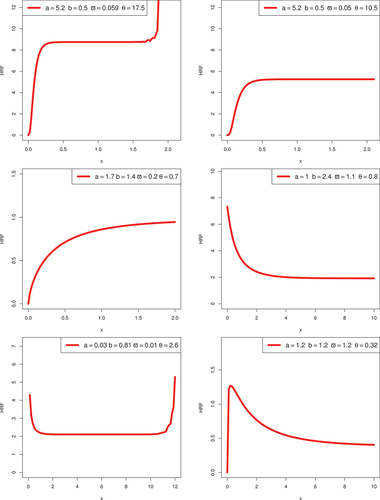
where $Q^{\mathrm{K}\mathrm{w}}\left(p\right)={\left[1-{\left(1-p\right)}^{\frac{1}{b}}\right]}^{\frac{1}{a}}$, denotes the QF of Kumaraswamy distribution (Kw) and $p\in [0,1]$. Some possible HRF and PDF shapes for the KwBE distribution are shown in Figures 1 and 2. These figures illustrate that the KwBE distribution’s PDF can be symmetric, reversed-J-shaped and right-skewed. In general, failure of various engineering systems after a bathtub HRF initially has to decrease, then a relatively static or useful life period and finally, an increasing failure rate. In the context of reliability theory, these three phases are known as burning, random, and wear-out failure zones (Liao et al., 2020). The plots of HRF are showing some flexible shapes, including increasing, decreasing, upside-down bathtub-shaped, and reversed bathtub-shaped, which quantifies the lifetime distribution features. It has a long constant failure rate period, which makes it possible to represent the second phase of the bathtub-shaped failure rate. Moreover, it also can effectively deal with the final stage of the bathtub-shaped failure rate. The flexibility in HRF of the proposed KwBE distribution can be used in a variety of social contexts.

Figure 1. Graphical illustration of PDF for some parametric values.

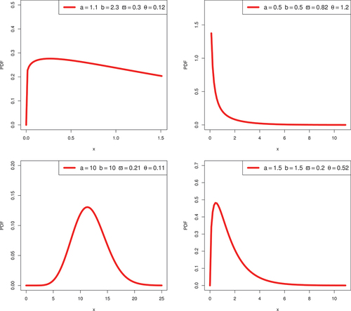
Figure 2. Graphical illustration of HRF for some parametric values.

2.1. Properties

Here, we derive a linear representation of the KwBG family, which is useful for acquiring several important properties of its submodels. Such representation will be used in the submodel of interest, KwBE distribution.

Proposition 2.2.

The linear functional representation of the KwBG family PDF and CDF is given by

(8) $f^{\mathrm{K}\mathrm{w}\mathrm{B}\mathrm{G}}\left(t;a,b,\varpi ,\xi \right)=\sum _{m=0}^{\mathrm{\infty }}{\mathrm{\Theta }}_m{f}_{m+1}\left(t\right)$(8)

and

(9) $F^{\mathrm{K}\mathrm{w}\mathrm{B}\mathrm{G}}\left(t;a,b,\varpi ,\xi \right)=\sum _{m=0}^{\mathrm{\infty }}{\mathrm{\Theta }}_m{F}_{m+1}\left(t\right),$(9)

respectively, where

(10) ${\mathrm{\Theta }}_m=\frac{ab\varpi e^{\varpi }}{{\left\{1-exp\left[1-e^{\varpi }\right]\right\}}^{a(1+v)}}\sum _{\nu =0}^{b-1}\sum _{\omega =0}^{a(1+v)-1}\sum _{n,i=0}^{\mathrm{\infty }}\frac{{\left(-1\right)}^{v+\omega +n+i+m}}{n!m!\left(m+1\right)}\left(\begin{array}{c}b-1\\ v\end{array}\right)$(10)

$\times \left(\begin{array}{c}a(1+v)-1\\ \omega \end{array}\right)\left(\begin{array}{c}n\\ i\end{array}\right){\left[(1+\omega )e^{\varpi }\right]}^n{\left[(i+1)\varpi \right]}^m,$

noting $F_{m+1}\left(t\right)=G{\left(t\right)}^{m+1}$ and $f_{m+1}\left(t\right)=(m+1)g(t)G(t{)}^{(m+1)-1}$ are the CDF and PDF, respectively, of the exp-G family with power parameter $(m+1)$.

Here, we use two series binomial expansion and power series for the exponential functions to obtain the linear representation of the KwBG family of distributions as follows:

(11) $(1-w{)}^z=\sum _{i=0}^{\mathrm{\infty }}(-1{)}^i\left(\begin{array}{c}z\\ i\end{array}\right)w^i,$(11)

where $(\begin{array}{c}z\\ i\end{array})$ represents the generalized binomial coefficients. The formula remains valid for $w$ such that $|w|<1$ only and

(12) $exp(-a{x}^b)=\sum _{v=0}^{\mathrm{\infty }}(-1{)}^v{a}^v\frac{x^{vb}}{v!},$(12)

for any real numbers $a$, $b$ and $x$, respectively (Alanzi et al., 2023).

Proof.

Let $T\sim \mathrm{K}\mathrm{w}\mathrm{B}\mathrm{G}(t;a,b,\varpi ,\xi )$ for $t>0$ and $a,b,\varpi ,\xi >0$; then its PDF is given by

(13) $f^{\mathrm{K}\mathrm{w}\mathrm{B}\mathrm{G}}\left(t;a,b,\varpi ,\xi \right)=ab\varpi g(t)exp\left\{\varpi \left[1-G(t)\right]\right\}exp\left\{-e^{\varpi }\left[1-e^{-\varpi G(t)}\right]\right\}\times {\left\{1-exp\left[1-e^{\varpi }\right]\right\}}^{-a}{\left\{1-exp\left(-e^{\varpi }\left[1-e^{-\varpi G(t)}\right]\right)\right\}}^{a-1}\times {\left[1-{\left\{\frac{1-exp\left(-e^{\varpi }\left[1-e^{-\varpi G(t)}\right]\right)}{1-exp(1-e^{\varpi })}\right\}}^a\right]}^{b-1}.$(13)

By using binomial expansion in (13), we obtained

(14) $\begin{array}{rl}& f^{\mathrm{K}\mathrm{w}\mathrm{B}\mathrm{G}}\left(t;a,b,\varpi ,\xi \right)=ab\varpi \sum _{\nu =0}^{b-1}\sum _{\omega =0}^{a(1+v)-1}{\left(-1\right)}^{v+\omega }\left(\begin{array}{c}b-1\\ v\end{array}\right)\left(\begin{array}{c}a(1+v)-1\\ \omega \end{array}\right)g(t)exp\left\{\varpi \left[1-G(t)\right]\right\}\\ & \times exp\left\{-(1+\omega )e^{\varpi }\left[1-e^{-\varpi G(t)}\right]\right\}{\left\{1-exp\left[1-e^{\varpi }\right]\right\}}^{-a(1+v)},\end{array}$(14)

using power series for exponential function (Alanzi et al., 2023; Bourguignon et al., 2014)

(15) $\begin{array}{rl}& f^{\mathrm{K}\mathrm{w}\mathrm{B}\mathrm{G}}\left(t;a,b,\varpi ,\xi \right)=ab\varpi \sum _{\nu =0}^{b-1}\sum _{\omega =0}^{a(1+v)-1}\sum _{n=0}^{\mathrm{\infty }}\frac{{\left(-1\right)}^{v+\omega +n}}{n!}\left(\begin{array}{c}b-1\\ v\end{array}\right)\left(\begin{array}{c}a(1+v)-1\\ \omega \end{array}\right){\left[(1+\omega )e^{\varpi }\right]}^n\times \\ & g(t)exp\left\{\varpi \left[1-G(t)\right]\right\}{\left\{1-exp\left[1-e^{\varpi }\right]\right\}}^{-a(1+v)}{\left[1-e^{-\varpi G(t)}\right]}^n,\end{array}$(15)

again using binomial expansion to the last term of Equation (15)(15) $\begin{array}{rl}& f^{\mathrm{K}\mathrm{w}\mathrm{B}\mathrm{G}}\left(t;a,b,\varpi ,\xi \right)=ab\varpi \sum _{\nu =0}^{b-1}\sum _{\omega =0}^{a(1+v)-1}\sum _{n=0}^{\mathrm{\infty }}\frac{{\left(-1\right)}^{v+\omega +n}}{n!}\left(\begin{array}{c}b-1\\ v\end{array}\right)\left(\begin{array}{c}a(1+v)-1\\ \omega \end{array}\right){\left[(1+\omega )e^{\varpi }\right]}^n\times \\ & g(t)exp\left\{\varpi \left[1-G(t)\right]\right\}{\left\{1-exp\left[1-e^{\varpi }\right]\right\}}^{-a(1+v)}{\left[1-e^{-\varpi G(t)}\right]}^n,\end{array}$(15) , we get

$f^{\mathrm{K}\mathrm{w}\mathrm{B}\mathrm{G}}\left(t;a,b,\varpi ,\xi \right)=\frac{ab\varpi e^{\varpi }}{{\left\{1-exp\left[1-e^{\varpi }\right]\right\}}^{a(1+v)}}\sum _{m=0}^{\mathrm{\infty }}\sum _{\nu =0}^{b-1}\sum _{\omega =0}^{a(1+v)-1}\sum _{n=0}^{\mathrm{\infty }}\sum _{i=0}^{\mathrm{\infty }}\frac{{\left(-1\right)}^{v+\omega +n+i+m}}{n!m!}\times \left(\begin{array}{c}b-1\\ v\end{array}\right)\left(\begin{array}{c}a(1+v)-1\\ \omega \end{array}\right)\left(\begin{array}{c}n\\ i\end{array}\right){\left[(1+\omega )e^{\varpi }\right]}^n{\left[(i+1)\varpi \right]}^{m}g(t)G(t{)}^m.$

The desired expression is obtained for $f^{\mathrm{K}\mathrm{w}\mathrm{B}\mathrm{G}}\left(t;a,b,\varpi ,\xi \right)$. The expression for $F^{\mathrm{K}\mathrm{w}\mathrm{B}\mathrm{G}}\left(t;a,b,\varpi ,\mathbf{x}\right)$ is obtained upon integral. This ends the proof of Proposition 2.2.□

Proposition 2.3.

Let $T\sim KwBE(t;a,b,\varpi ,\theta )$ for $t>0$ and $a,b,\varpi ,\theta >0$, then a linear representation of the KwBE model by using Eq.(8) is as follows:

(16) $f^{\mathrm{K}\mathrm{w}\mathrm{B}\mathrm{E}}\left(t;a,b,\varpi ,\theta \right)=\sum _{h=0}^{\mathrm{\infty }}{\mathrm{\Theta }}_h\pi \left[t;\theta (h+1)\right],$(16)

where ${\mathrm{\Theta }}_h={\sum }_{m=0}^{\mathrm{\infty }}{\mathrm{\Theta }}_m{\left(-1\right)}^h\left(\begin{array}{c}m\\ h\end{array}\right)(m+1)(h+1{)}^{-1}$ and ${\mathrm{\Theta }}_m$ is defined in Proposition 2.2.

Proof.

By using Eq.(8) and binomial expansion, we get

(17) $f^{\mathrm{K}\mathrm{w}\mathrm{B}\mathrm{E}}\left(t;a,b,\varpi ,\theta \right)=\left(m+1\right)\sum _{h=0}^{\mathrm{\infty }}\sum _{m=0}^{\mathrm{\infty }}{\mathrm{\Theta }}_m{\left(-1\right)}^h\left(\begin{array}{c}m\\ h\end{array}\right)\theta e^{-\theta t(1+h)}.$(17)

The desired result is obtained for $f^{\mathrm{K}\mathrm{w}\mathrm{B}\mathrm{E}}\left(t;a,b,\varpi ,\theta \right)$. This completes the proof of Proposition 2.3. □

Form Eq.(16), we see that the PDF of the KwBE model can be expressed as an infinite general linear mixture of PDFs of the exponential model. Therefore, several significant properties of the KwBE model can be deduced from the exponential model by using Eq.(16), where $\pi \left[t;\theta (h+1)\right]$ is an exp-exponential PDF with parameter $\theta (h+1)$.

2.2. Th moment

The mean and variance of the KwBE distribution can be obtained by using Eq. (18), where that is mean=${\mu }_1^{\prime }$ and variance=${\mu }_2$=${\mu }_2^{\prime }-{\left({\mu }_1^{\prime }\right)}^2.$ Moreover, the first four actual moments can be obtained using the well-established relationship between ordinary and mean moments. The moment-based measure of skewness and kurtosis, respectively, is obtained by using ${\beta }_1=\frac{{\mu }_3^2}{{\mu }_2^3}$ and ${\beta }_2=\frac{{\mu }_4}{{\mu }_2^2}$, where ${\mu }_3={\mu }_3^{\prime }-3{\mu }_2^{\prime }{\mu }_1^{\prime }+2({\mu }_1^{\prime }{)}^3$and ${\mu }_4={\mu }_4^{\prime }-4{\mu }_3^{\prime }{\mu }_1^{\prime }+6{\mu }_2^{\prime }({\mu }_1^{\prime }{)}^2-3({\mu }_1^{\prime }{)}^4$. Pearson’s coefficient of skewness and kurtosis can be yielded as $\sqrt{{\beta }_1}$ and ${\beta }_2-3$, respectively. The $r$th raw or ordinary moment of the KwBE distribution is given by

(18) ${\mu }_r^{\prime }=\frac{1}{{\theta }^r}\mathrm{\Gamma }\left(r+1\right)\sum _{h=0}^{\mathrm{\infty }}{\mathrm{\Theta }}_h(h+1{)}^{-r}.$(18)

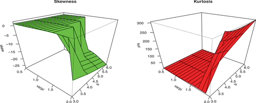
The graphical illustration of mean and variance at varying parameters to underline the effect of parameters is presented in Figures 3–4. It is obvious from Figure 3 that as the value of parameter $a$ and $\varpi$ increase, the mean and variance tend to decrease for fixed parameter $b=7$ and scale parameter $\theta =1$. However, from Figure 5–6, the skewness and kurtosis of the KwBE distribution tend to rise as the values of parameter $a$ and $\varpi$ increase.

Figure 3. Graphical illustration of mean and variance of the KwBE distribution for $a\in (1.5:5.5)$, $\theta =1$, $b=7$ and $\varpi \in (0.10:5.0)$.

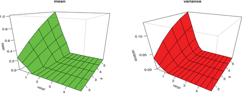
Figure 4. Graphical illustration of mean and variance of the KwBE distribution for $a=5$, $\theta =1$, $b\in (1.5:5.5)$ and $\varpi \in (0.10:5.0)$.

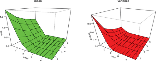
Figure 5. Graphical illustration of skewness and kurtosis of the KwBE distribution for $a\in (5:30)$, $\theta =0.20$, $b=2$ and $\varpi \in (0.50:2.0)$.

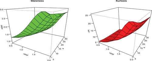
Figure 6. Graphical illustration of skewness and kurtosis of the KwBE distribution for $a=7$, $\theta =0.30$, $b\in (3:6)$ and $\varpi \in (0.50:2.0)$.

2.3. Moment generating function

The MGF of a real-valued random variable in probability theory and statistics is an effective way to describe its probability distribution. Let T be a random variable with PDF $f(t)$. The MGF is defined by $M_z(t)=E(e^{zt})=\underset{-\mathrm{\infty }}{\overset{+\mathrm{\infty }}{\int }}{e}^{zt}f(t)dt$.

Proposition 2.4.

Let T $\sim$ $KwBE(t;a,b,\varpi ,\theta )$ for $t>0$ and $a,b,\varpi ,\theta >0$. Then its MGF using Wright generalized hypergeometric function Erdélyi, (1953) by is as follows:

(19) $M_z(t)=\sum _{h=0}^{\mathrm{\infty }}{\mathrm{\Theta }}_h{{\left[\theta (h+1)\right]}^{-m}}_1{\psi }_0\left[\begin{array}{c}1,1\\ -\end{array};z\right].$(19)

Proof.

The Wright generalized hypergeometric function holds $\left(p=q+1,|t|<1\right)$ is given by

(20) ${ }_p{\psi }_q\left[\begin{array}{cc}\left({\alpha }_1,A_1\right),\cdots \cdots ,& \left({\alpha }_p,A_p\right)\\ \left({\beta }_1,B_1\right),\cdots \cdots ,& \left({\beta }_q,B_q\right)\end{array};t\right]=\sum _{n=0}^{\mathrm{\infty }}\frac{{\prod }_{j=1}^p\mathrm{\Gamma }\left({\alpha }_j+A_{j}n\right)}{{\prod }_{j=1}^q\mathrm{\Gamma }\left({\beta }_j+B_{j}n\right)}\frac{t^n}{n!}.$(20)

Using Equation (16)(16) $f^{\mathrm{K}\mathrm{w}\mathrm{B}\mathrm{E}}\left(t;a,b,\varpi ,\theta \right)=\sum _{h=0}^{\mathrm{\infty }}{\mathrm{\Theta }}_h\pi \left[t;\theta (h+1)\right],$(16) , and by definition of the MGF and expanding $e^{zt}={\sum }_{m=0}^{\mathrm{\infty }}\frac{z^m}{m!}{t}^m$, we get

$M_z(t)=\theta (h+1)\sum _{h=0}^{\mathrm{\infty }}{\mathrm{\Theta }}_h\sum _{m=0}^{\mathrm{\infty }}\underset{0}{\overset{\mathrm{\infty }}{\int }}\frac{z^m}{m!}{t}^m{e}^{-\theta (h+1)t}dt,$

after simplification and using Eq. (20) in Eq. (21), we get

(21) $M_z(t)=\sum _{h=0}^{\mathrm{\infty }}{\mathrm{\Theta }}_h\frac{1}{{\left(\theta (h+1)\right)}^m}\sum _{m=0}^{\mathrm{\infty }}\frac{z^m}{m!}\mathrm{\Gamma }\left(m+1\right).$(21)

This ends the proof of Proposition 2.4.

2.4. Réyni entropy

As a measure of diversity, the Rényi entropy (RE) is significant in ecology and statistics. It is also significant in the field of quantum information because it may be used to quantify entanglement. It was given by Alfréd Rényi, a Hungarian mathematician.

Proposition 2.5.

The functional linear representation of the RE of the KwBG family is given by

(22) $R_{\delta }\left(t\right)={\left(1-\delta \right)}^{-1}log\left[\sum _{\vartheta =0}^{\mathrm{\infty }}{\kappa }_{\vartheta }\underset{-\mathrm{\infty }}{\overset{+\mathrm{\infty }}{\int }}g{(t)}^{\delta }G{(t)}^{\vartheta }dt\right],$(22)

where

(23) ${\kappa }_{\vartheta }=\frac{{\left(ab\varpi \right)}^{\delta }{e}^{\delta \varpi }}{{\left[1-exp\left(1-e^{\varpi }\right)\right]}^{a\left(\delta +\mathrm{\hslash }\right)}}\sum _{\mathrm{\hslash }=0}^{\delta \left(b-1\right)}\sum _{\mathrm{\wp }=0}^{\delta \left(a-1\right)+a\mathrm{\hslash }}\sum _{n=0}^{\mathrm{\infty }}\sum _{z=0}^{\mathrm{\infty }}\frac{{\left(-1\right)}^{\mathrm{\hslash }+\mathrm{\wp }+n+z+\vartheta }}{n!\vartheta !}\times \left(\begin{array}{c}n\\ z\end{array}\right){\left[(\mathrm{\wp }+\delta )e^{\varpi }\right]}^n{\left[(\delta +z)\varpi \right]}^{\vartheta }\left(\begin{array}{c}\delta \left(b-1\right)\\ \mathrm{\hslash }\end{array}\right)\left(\begin{array}{c}\delta \left(a-1\right)+a\mathrm{\hslash }\\ \mathrm{\wp }\end{array}\right).$(23)

Let X $\sim$ follows the KwBE model, using the Proposition 2.5, the RE is given by

(24) $R_{\delta }\left(t\right)={\left(1-\delta \right)}^{-1}log\left[\sum _{d=0}^{\mathrm{\infty }}{\kappa }_d\frac{{\theta }^{\delta -1}}{(\delta +d)}\right],$(24)

where ${\kappa }_d={\sum }_{\vartheta =0}^{\mathrm{\infty }}{\kappa }_{\vartheta }{\left(-1\right)}^d\left(\begin{array}{c}\delta \\ d\end{array}\right)$ and ${\kappa }_{\vartheta }$ is defined in Equation (23)(23) ${\kappa }_{\vartheta }=\frac{{\left(ab\varpi \right)}^{\delta }{e}^{\delta \varpi }}{{\left[1-exp\left(1-e^{\varpi }\right)\right]}^{a\left(\delta +\mathrm{\hslash }\right)}}\sum _{\mathrm{\hslash }=0}^{\delta \left(b-1\right)}\sum _{\mathrm{\wp }=0}^{\delta \left(a-1\right)+a\mathrm{\hslash }}\sum _{n=0}^{\mathrm{\infty }}\sum _{z=0}^{\mathrm{\infty }}\frac{{\left(-1\right)}^{\mathrm{\hslash }+\mathrm{\wp }+n+z+\vartheta }}{n!\vartheta !}\times \left(\begin{array}{c}n\\ z\end{array}\right){\left[(\mathrm{\wp }+\delta )e^{\varpi }\right]}^n{\left[(\delta +z)\varpi \right]}^{\vartheta }\left(\begin{array}{c}\delta \left(b-1\right)\\ \mathrm{\hslash }\end{array}\right)\left(\begin{array}{c}\delta \left(a-1\right)+a\mathrm{\hslash }\\ \mathrm{\wp }\end{array}\right).$(23) .

Proof.

By using (22) and considering $\mathrm{I}={\int }_{-\mathrm{\infty }}^{+\mathrm{\infty }}g{(t)}^{\delta }G(t{)}^{\vartheta }dt$

$\mathrm{I}=\underset{-\mathrm{\infty }}{\overset{+\mathrm{\infty }}{\int }}\sum _{d=0}^{\mathrm{\infty }}{\left(-1\right)}^d\left(\begin{array}{c}\vartheta \\ d\end{array}\right){\theta }^{\delta }{e}^{-\theta t(\delta +d)}dt,$

after simplification, we get

(25) $\mathrm{I}=\sum _{d=0}^{\mathrm{\infty }}{\left(-1\right)}^d\left(\begin{array}{c}\vartheta \\ d\end{array}\right){\theta }^{\delta }\frac{1}{\theta (\delta +d)}.$(25)

By replacing Equation (25)(25) $\mathrm{I}=\sum _{d=0}^{\mathrm{\infty }}{\left(-1\right)}^d\left(\begin{array}{c}\vartheta \\ d\end{array}\right){\theta }^{\delta }\frac{1}{\theta (\delta +d)}.$(25) in Equation (22)(22) $R_{\delta }\left(t\right)={\left(1-\delta \right)}^{-1}log\left[\sum _{\vartheta =0}^{\mathrm{\infty }}{\kappa }_{\vartheta }\underset{-\mathrm{\infty }}{\overset{+\mathrm{\infty }}{\int }}g{(t)}^{\delta }G{(t)}^{\vartheta }dt\right],$(22) , yields the desired result and completes the proof.□

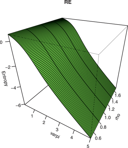
The graphical illustration of RE is presented in Figure 7, by setting $\varpi \in (1:5)$, $\theta =0.50$, $b=5$, $a\in (2:6)$ and $\delta \in (0.5:1.7).$ The effect of parameter $\varpi$ and $\delta$ and RE is negatively associated and indicated that as $\varpi$ and $\delta$ increases, the RE tends to decrease. Moreover, it shows flexibility under the KwBE model because it yields both positive and negative values.

Figure 7. Plot of RE for some parametric values.

3. Estimation with a simulation study

Let $t_1,t_2,\cdots ,t_n$ be the observed values of a random sample of size $n$ from the KwBGE model. Then, the log-likelihood function of the parameter vector $\mathrm{\varnothing }={\left(a,b,\varpi ,\theta \right)}^T$ is as follows:

(26) $\begin{array}{rl}& \mathrm{\ell }\left(\mathrm{\varnothing }\right)=nlog\left(ab\varpi \theta \right)-\theta \sum _{i=1}^n{t}_i+\varpi \sum _{i=1}^n\left[1-\left(1-e^{-\theta t_i}\right)\right]-e^{\varpi }\sum _{i=1}^n\left[1-e^{-\varpi \left(1-e^{-\theta t_i}\right)}\right]\\ & +\left(a-1\right)\sum _{i=1}^{n}log\left[1-exp\left(-e^{\varpi }\left[1-e^{-\varpi \left(1-e^{-\theta t_i}\right)}\right]\right)\right]-nalog\left[1-exp\left(1-e^{\varpi }\right)\right]\\ & +\left(b-1\right)\sum _{i=1}^{n}log\left(1-{\left\{\frac{1-exp\left(-e^{\varpi }\left[1-e^{-\varpi \left(1-e^{-\theta t_i}\right)}\right]\right)}{1-exp(1-e^{\varpi })}\right\}}^a\right).\end{array}$(26)

By partially differentiating Equation (26)(26) $\begin{array}{rl}& \mathrm{\ell }\left(\mathrm{\varnothing }\right)=nlog\left(ab\varpi \theta \right)-\theta \sum _{i=1}^n{t}_i+\varpi \sum _{i=1}^n\left[1-\left(1-e^{-\theta t_i}\right)\right]-e^{\varpi }\sum _{i=1}^n\left[1-e^{-\varpi \left(1-e^{-\theta t_i}\right)}\right]\\ & +\left(a-1\right)\sum _{i=1}^{n}log\left[1-exp\left(-e^{\varpi }\left[1-e^{-\varpi \left(1-e^{-\theta t_i}\right)}\right]\right)\right]-nalog\left[1-exp\left(1-e^{\varpi }\right)\right]\\ & +\left(b-1\right)\sum _{i=1}^{n}log\left(1-{\left\{\frac{1-exp\left(-e^{\varpi }\left[1-e^{-\varpi \left(1-e^{-\theta t_i}\right)}\right]\right)}{1-exp(1-e^{\varpi })}\right\}}^a\right).\end{array}$(26) with respect to $\mathrm{\varnothing }={\left(a,b,\varpi ,\theta \right)}^T$, we obtain the log-likelihood equations of $\frac{\mathrm{\partial }\mathrm{\ell }\left(\mathrm{\varnothing }\right)}{\mathrm{\partial }a}$,$\frac{\mathrm{\partial }\mathrm{\ell }\left(\mathrm{\varnothing }\right)}{\mathrm{\partial }b}$, $\frac{\mathrm{\partial }\mathrm{\ell }\left(\mathrm{\varnothing }\right)}{\mathrm{\partial }\varpi }$ and $\frac{\mathrm{\partial }\mathrm{\ell }\left(\mathrm{\varnothing }\right)}{\mathrm{\partial }\theta }$. Thus, we obtain a system of equations with no explicit solution. Consequently, it needs computer power to use nonlinear numerical approximation methods (quasi Newton-Raphson) to get the maximum likelihood estimators. The partial derivatives of the log-likelihood equations are presented in the appendix.

3.1. Simulation

In this section, a simulation study is carried out to compare the performance of the maximum likelihood estimates of the unknown parameters for the KwBE $(a,b,\varpi ,\theta )$ distribution and analysis outcomes are graphically presented in Figures 8 and 9. The following procedure is adopted to perform a Monte Carlo simulation:

1. first, choose the starting values for the parameters $a,b,\varpi ,\theta$ and determine the sample size, we consider the initial values as follows $a=1.20$, $b=0.85$, $\varpi =1.80$ and $\theta =0.32$;

2. generate a random sample of size $n$ for the KwBE distribution, we consider various sample sizes $n=20$, $n=25$,$\cdots$, $n=250$;

3. calculate the estimates of the KwBE distribution, mean square errors (MSEs) and biases. The following formulas are used to compute the two accuracy measures (MSEs and biases

   $\mathrm{B}\mathrm{i}\mathrm{a}{\mathrm{s}}_{\upsilon }=\frac{1}{1000}\sum _{i=1}^{1000}\left({\hat{\upsilon }}_i-\upsilon \right)\mathrm{a}\mathrm{n}\mathrm{d}\mathrm{M}\mathrm{S}{\mathrm{E}}_{\upsilon }=\frac{1}{1000}\sum _{i=1}^{1000}{\left({\hat{\upsilon }}_i-\upsilon \right)}^2,$
   respectively (for $\upsilon =a,b,\varpi ,\theta$);

4. replicate the steps (ii) and (iii) $N$ times.

Figure 8. Graphical illustration of biases at varying sample sizes.

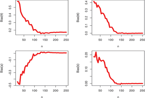
Figure 9. Graphical illustration of MSEs at varying sample sizes.

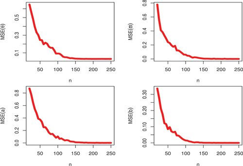
It is obvious form Figures 8 and 9, as $n$ increases, both the empirical biases and MSEs tend to zero in all cases for parameter $a,b,\varpi$ and $\theta$.

4. GASP based on the KwBE model

4.1. Construction

This section emphasizes an optimization of design parameters namely $c$ (acceptance number) and $g$ (group size or total number of groups) for truncated life test experiments to accept or reject the lot under investigation. The GASP helps not only minimize the lot inspection duration by considering a variety of items on a single tester but cost-effective. A GASP offers a stricter product inspection than an ordinary ASP because samples are divided among distinct groups. Here, we use the median as a quality index as the QF of the KwBE model that has an elegant closed-form solution. On the other side, it is well established that the median life test for skewed models yields better outputs than mean (Aslam et al., 2011). The construction of ASP using multiple items on a single tester is based on the following steps:

• First, choose the number of groups g and assign preset r (group size) items to each group. Thus, the size of the lot will be $n=gr$.

• Second, choose the $c$ and the experiment time ($t_0$).

• Third, run the experiment simultaneously for each of the $g$ groups and count the number of failures for each group.

• Finally, the lot under investigation is accepted if the number of failures does not exceed the acceptance number c.

Assume that for any lot, the median life of the products, say $m$, exceeds the required life, say $m_0$. We will accept the lot if there is sufficient evidence that $m>m_0$ is at particular levels of producer and consumer risks. Then the lot’s acceptance probability is determined by

(27) $p_{a\left(p\right)}={\left[\sum _{i=0}^c\left(\begin{array}{c}r\\ i\end{array}\right)p^i{\left[1-p\right]}^{r-i}\right]}^g,$(27)

where $p$ denotes the likelihood that an item in a group would fail before $t_0$ and it is determined by substituting Eq. (7) in Eq. (5). But first, we need to evaluate the value of parameters $\theta$ and $t$. Let assume $m=Q_p$

(28) $m=-\frac{1}{\theta }ln\left[1-\left\{1-{\lambda }^{-1}ln\left[ln\left(1-\left[1-exp(1-e^{\lambda })\right]\left[Q^{\mathrm{K}\mathrm{w}}\left(p\right)\right]\right)+exp(\lambda )\right]\right\}\right],$(28)

where $Q_p$ is given in (7), and consider

$\zeta =ln\left[1-\left\{1-{\lambda }^{-1}ln\left[ln\left(1-\left[1-exp(1-e^{\lambda })\right]\left[Q^{\mathrm{K}\mathrm{w}}\left(0.5\right)\right]\right)+exp(\lambda )\right]\right\}\right],$

which implies $\theta =-\zeta \text{overm}$ and $t=m_0{a}_1,$ by replacing $\theta$, $t$ and $r_2=\frac{m}{m_0}$ in Eq. (5) and the probability of failure based on the KwBE model can be expressed as follows:

(29) $p=1-{\left[1-{\left\{\frac{1-exp\left\{-e^{\varpi }\left[1-e^{-\varpi \left[1-e^{a_1\zeta {\left(r_2\right)}^{-1}}\right]}\right]\right\}}{1-exp(1-e^{\varpi })}\right\}}^a\right]}^b.$(29)

When $a_1$ and $r_2$ = $m/m_0$ are predefined, the probability of failure under the KwBE model, $p$ can be calculated for selected parametric values for $a$ and $b$. Moreover, the operating characteristic (OC) function $P_{(a)}$ requires that the following two inequalities be satisfied simultaneously to determine the design parameters $g$ and $c$. While $r_1$ and $r_2$ denote the ratio at the consumer’s risk (here, it is considered to be 1) and the ratio at the producer’s risk, respectively

(30) $p_{a\left(p_1|\frac{m}{m_0}=r_1\right)}={\left[\sum _{i=0}^c\left(\begin{array}{c}r\\ i\end{array}\right)p_1^i{\left[1-p_1\right]}^{r-i}\right]}^g\le \beta ,$(30)

and

(31) $p_{a\left(p_2|\frac{m}{m_0}=r_2\right)}={\left[\sum _{i=0}^c\left(\begin{array}{c}r\\ i\end{array}\right)p_2^i{\left[1-p_2\right]}^{r-i}\right]}^g\ge 1-\gamma .$(31)

The failure probabilities that are associated to both consumer’s ($\beta$) and producer’s ($\gamma$) risk, denoted by $p_1$ and $p_2$ can be evaluated based on the KwBE model using Eq. (32) and Eq. (33), respectively, and can be applied in Eq. (30) and Eq. (31).

(32) $p_1=1-{\left[1-{\left\{\frac{1-exp\left\{-e^{\varpi }\left[1-e^{-\varpi \left[1-e^{a_1\zeta }\right]}\right]\right\}}{1-exp(1-e^{\varpi })}\right\}}^a\right]}^b$(32)

and

(33) $p_2=1-{\left[1-{\left\{\frac{1-exp\left\{-e^{\varpi }\left[1-e^{-\varpi \left[1-e^{a_1\zeta {\left(r_2\right)}^{-1}}\right]}\right]\right\}}{1-exp(1-e^{\varpi })}\right\}}^a\right]}^b.$(33)

4.2. Discussion

Tables 2 and 3 illustrate the design parameters under GASP based on the KwBE distribution for various values of $\varpi$ (1.25 and 1.5). The two-level of $r$ (5, 10) is considered. From Table 2, it is determined that a decrease in consumer risk ($\beta$), results in a rise in the number of groups ($g$), for instance, when $\beta$ = 0.25 with true median life $r_2$ = 4 evaluates $g=40$, similarly by reducing $\beta$ = 0.25 to $\beta$ = 0.01 yields $g$ = 131. Additionally, the $g$ size rapidly reduces as $r_2$ rises. Table 2 shows the impact of termination ratio, $a_1$ = 0.5 and revealed that when $\beta =0.25$, $r_2$ = 4, $a_1$ = 0.5 and $r$ = 5, it requires to put total 200 ($40\times 5$) units on a life test. Similar to this, by increasing $r$ = 10, a considerable decrease in the overall number of units for life testing from 200 to 30 can be seen. As a result, in this case, 10 groups will be preferred because it tends to save enough cost and time. From Table 1–2, when the $r_2$ increases for the GASP under consideration, the size of $g$ drops and the value of operating characteristic (OC) function increases for the KwBE distribution using median lifetime as the quality index, when $\beta$ = 0.01, $a_1$ = 1, $\varpi$ = 1.25, and for $r$ = 10.

Table 1. Proposed GASP based on the KwBE model

$r_2$	2	4	6	8
$n$	–	100	50	30
$g$	–	10	5	3
$c$	–	5	4	3
$P(a)$	–	0.9688	0.9803	0.9838

Table 2. A GASP under the KwBE model, $a=1.00$, $b=1.00$, $\varpi =1.25$

	$\mathit{r}\mathbf{=}\mathbf{5}$							$\mathit{r}\mathbf{=}\mathbf{10}$
		${\mathit{a}}_{\mathbf{1}}\mathbf{=}\mathbf{0.5}$			${\mathit{a}}_{\mathbf{1}}\mathbf{=}\mathbf{5}$			${\mathit{a}}_{\mathbf{1}}\mathbf{=}\mathbf{0.5}$			${\mathit{a}}_{\mathbf{1}}\mathbf{=}\mathbf{1}$
$\beta$	${\mathit{r}}_{\mathbf{2}}$	$\mathit{g}$	$\mathit{c}$	$\mathit{p}(a)$	$\mathit{g}$	$\mathit{c}$	$\mathit{p}(a)$	$\mathit{g}$	$\mathit{c}$	$p(a)$	$\mathit{g}$	$\mathit{c}$	$\mathit{p}(a)$
0.25	2	–	–	–	–	–	–	–	–	–	–	–	–
	4	40	3	0.9860	7	3	0.9721	3	3	0.9701	2	4	0.9624
	6	8	2	0.9815	3	2	0.9559	2	2	0.9565	1	3	0.9748
	8	8	2	0.9917	3	2	0.979	2	2	0.9792	1	3	0.9899
0.1	2	–	–	–	–	–	–	–	–	–	–	–	–
	4	66	3	0.9770	12	3	0.9527	5	3	0.9507	5	5	0.9843
	6	12	2	0.9724	12	3	0.9881	5	3	0.9875	2	3	0.9503
	8	12	2	0.9875	4	2	0.9721	3	2	0.9689	2	3	0.9800
0.05	2	–	–	–	–	–	–	–	–	–	–	–	–
	4	85	3	0.9705	95	4	0.9845	17	3	0.9798	7	5	0.9781
	6	16	2	0.9633	15	3	0.9852	7	3	0.9825	2	3	0.9503
	8	16	2	0.9834	5	2	0.9652	3	2	0.9689	2	3	0.9800
0.01	2	–	–	–	–	–	–	–	–	–	–	–	–
	4	131	3	0.9549	146	4	0.9763	26	4	0.9693	10	5	0.9688
	6	131	3	0.9899	23	3	0.9774	10	3	0.9751	5	4	0.9803
	8	24	2	0.9752	7	2	0.9517	10	3	0.991	3	3	0.9838

Remark: Hyphens (–) are inserted in required cells for a large sample size.

Here, we reveal the hypothetical example and assume that the producer believes that the specified value of $m_0$ = 2000 hours, the lifetime of the units follows the KwBE distribution with $\varpi$ = 1.50, the risk to the consumer, and the producer are 0.25 and 0.05, respectively, whereas the group size is $r$ = 5, and the actual value of $m$ is 8000 hours. An experimenter wishes to conduct a life test experiment for 1000 hours and for that, we are interested in formulating GASP for $a_1$ = 0.5, $\beta$ = 0.25, and true median life ($\frac{m}{m_0}$) = 4. For the given information and using Table 3, the design parameters $g$ and $c$ can be obtained as $g$ = 41 and $c$ = 3. As a result, a sample of size 205 $(41\times 5)$ should be collected, and each of the 41 groups should get 5 units. If there are no more than three units that fail in any group before 1000 hours, the lot is eventually accepted; if there are more than three, the lot is rejected.

Table 3. A GASP under the KwBE model, $a=1.00$, $b=1.00$, $\varpi =1.50$

	$\mathit{r}\mathbf{=}\mathbf{5}$							$\mathit{r}\mathbf{=}\mathbf{10}$
		$\mathit{r}\mathbf{=}\mathbf{5}$			$\mathit{r}\mathbf{=}\mathbf{10}$			${\mathit{a}}_{\mathbf{1}}\mathbf{=}\mathbf{0.5}$			${\mathit{a}}_{\mathbf{1}}\mathbf{=}\mathbf{5}$
$\beta$	${\mathit{r}}_{\mathbf{2}}$	$\mathit{g}$	$\mathit{c}$	$\mathit{p}(a)$	$\mathit{g}$	$\mathit{c}$	$\mathit{p}(a)$	$\mathit{g}$	$\mathit{c}$	$p(a)$	$\mathit{g}$	$\mathit{c}$	$\mathit{p}(a)$
0.25	2	–	–	–	–	–	–	–	–	–	–	–	–
	4	41	3	0.9866	7	3	0.9735	3	3	0.9718	2	4	0.9644
	6	8	2	0.9824	3	2	0.9578	2	2	0.9584	1	3	0.9761
	8	8	2	0.9921	3	2	0.9800	2	2	0.9802	1	3	0.9905
0.1	2	–	–	–	–	–	–	–	–	–	–	–	–
	4	68	3	0.9779	12	3	0.9550	5	3	0.9535	5	5	0.9854
	6	13	2	0.9715	12	3	0.9888	5	3	0.9883	2	3	0.9528
	8	13	2	0.9872	4	2	0.9734	3	2	0.9705	2	3	0.9811
0.05	2	–	–	–	–	–	–	–	–	–	–	–	–
	4	88	3	0.9715	95	4	0.9855	17	4	0.9814	7	5	0.9796
	6	16	2	0.9651	15	3	0.9861	7	3	0.9836	2	3	0.9528
	8	16	2	0.9843	5	2	0.9669	3	2	0.9705	2	3	0.9811
0.01	2	–	–	–	–	–	–	–	–	–	–	–	–
	4	135	3	0.9565	146	4	0.9778	26	4	0.9716	10	5	0.9709
	6	135	3	0.9903	23	3	0.9787	10	3	0.9767	5	4	0.9816
	8	25	2	0.9755	7	2	0.9540	5	2	0.9513	3	3	0.9718

Remark: Hyphens (–) are inserted in required cells for a large sample size.

5. Real-life applications

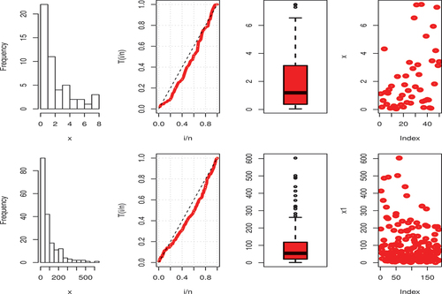
In this section, we use two failure time data sets to underline the usefulness of the proposed KwBE distribution. Recently, Almarashi et al. (Almarashi et al., 2021) used the Marshall-Olkin Kumaraswamy Exponential (MOKw-E) distribution and proposed GASP using the breaking stress of carbon fiber (in Gba) data. The following are the data, which consist of 50 observed values for the carbon fiber breaking stress: 1.120, 0.170, 0.640, 4.320, 1.220, 0.370, 1.160, 1.420, 0.090, 1.670, 0.130, 0.250, 0.080, 0.040, 2.350, 0.200, 0.780, 0.340, 1.020, 0.170, 1.760, 2.390, 0.500, 1.350, 3.360, 0.450, 0.900, 2.920, 6.530, 1.620, 7.460, 3.190, 2.490, 1.400, 7.490, 0.570, 0.140, 0.630, 5.230, 0.710, 0.680, 0.120, 0.090, 3.470, 5.930, 1.820, 4.200, 7.290, 3.130 and 3.41. Moreover, Almarashi et al. (Almarashi et al., 2021) fitted four-parameter MOKw-E distribution to the above data and the result revealed that the maximum distance between the sample’s empirical distribution function and the reference distribution’s CDF is 0.0681 with a p-value (PV) 0.9743. On the other side, the proposed KwBE distribution outperforms with the least Kolmogorov–Smirnov (KS) statistic 0.04531 and PV exactly 1 (see Table 5). The second set of data includes the total number of air conditioning system failures recorded by a fleet of 13 Boeing 720 aircraft (Kumar & Kumar, 2019) and the records were kept for how long each aircraft’s air conditioning system failed in succession. The aircraft had a meticulous overhaul after approximately 2000 hours of operation. The data are as follows: 194, 413, 90, 74, 55, 23, 97, 50, 359, 50, 130, 487, 57, 102, 15, 14, 10, 57, 320, 261, 51, 44, 9, 254, 493, 33, 18, 209, 41, 58, 60, 48, 56, 87, 11, 102, 12, 5, 14, 14, 29, 37, 186, 29, 104, 7, 4, 72, 270, 283, 7, 61, 100, 61, 502, 220, 120, 141, 22, 603, 35, 98, 54, 100, 11, 181, 65, 49, 12, 239, 14, 18, 39, 3, 12, 5, 32, 9, 438, 43, 134, 184, 20, 386, 182, 71, 80, 188, 230, 152, 5, 36, 79, 59, 33, 246, 1, 79, 3, 27, 201, 84, 27, 156, 21, 16, 88, 130, 14, 118, 44, 15, 42, 106, 46, 230, 26, 59, 153, 104, 20, 206, 5, 66, 34, 29, 26, 35, 5, 82, 31, 118, 326, 12, 54, 36, 34, 18, 25, 120, 31, 22, 18, 216, 139, 67, 310, 3, 46, 210, 57, 76, 14, 111, 97, 62, 39, 30, 7, 44, 11, 63, 23, 22, 23, 14, 18, 13, 34, 16, 18, 130, 90, 163, 208, 1, 24, 70, 16, 101, 52, 208, 95, 62, 11, 191, 14 and 71. Table 4 presents the descriptive information for both data sets and demonstrates that both are leptokurtic and skew to the right. The Shapiro–Wilk test also confirms that the samples do not come from a normal distribution as W (0.81505 and 0.74743) with PV less than 0.05, for the first and second data, respectively.

Table 4. Descriptive information of both data sets

Data	$\mathit{n}$	${\mathit{x}}_{\mathbf{0}}$	${\mathit{Q}}_{\mathbf{1}}$	$\tilde{\mathit{x}}$	$\bar{\mathit{x}}$	$\sigma$	${\mathit{Q}}_{\mathbf{3}}$	${\mathit{x}}_{\mathit{m}}$	S	K
First	50	0.040	0.390	1.190	1.975	2.116	3.078	7.490	1.325	3.803
Second	188	1.000	20.750	54.000	92.070	107.916	118.000	603.000	2.139	8.023

Figure 10 shows some basic characteristics of data by visually including histograms, TTT, box and index plots of the data sets. Both the data sets are right-skewed and the TTT plot indicates that the HRF of the data sets is increasing-decreasing-increasing.

Figure 10. Graphical illustration of first (top) and second (bottom) data.

Several extended or modified exponential-based distributions are compared with the proposed KwBE distribution, such as the KwPE distribution (Chakraborty et al., 2022), the exponentiated exponential (EE) distribution (Nadarajah, 2011), the Marshall-Olkin exponential (MOE) distribution (Marshall & Olkin, 1997), the exponentiated Weibull (EW) distribution (Mudholkar & Srivastava, 1993), the odd Weibull exponential (OWE) distribution (Bourguignon et al., 2014), the Kumaraswamy exponential (KE) distribution (Nadarajah et al., 2012), the beta exponential (BE) distribution (Jones, 2004), the Topp-Leone exponential (TLE) distribution (Al-Shomrani et al., 2016), the alpha power exponentiated exponential (APEE) (Afify et al., 2020) distribution, the transmuted exponentiated exponential (TEE) distribution (Khan et al., 2017), the gamma exponentiated exponential (GEE) distribution (Ristić & Balakrishnan, 2012), the exponentiated exponential Poisson (EEP) distribution (Pogány, 2015), the Weibull (W) distribution (Weibull, 1951) and the Nadarajah and Haghighi (NH) distribution (Nadarajah & Haghighi, 2011). Tables 5 and 6 show the estimated parameters (Esti.) along with standard error (S.E) of the estimates and goodness-of-fit statistics for both data sets. The proposed KwBE distribution provides better fits compared to several exponential-based extended models. Generally, the model is considered best if earlier statistics and the KS test have the least, but higher PV. For both data sets, the plots of estimated PDF and the CDF based on the KwBE distribution are shown in Figure 11, which support the goodness-of-fit measures given in Tables 5 and 6.

Figure 11. Graphical illustration of the estimated PDF and the CDF under the KwBE model, first (top) and second (bottom) data.

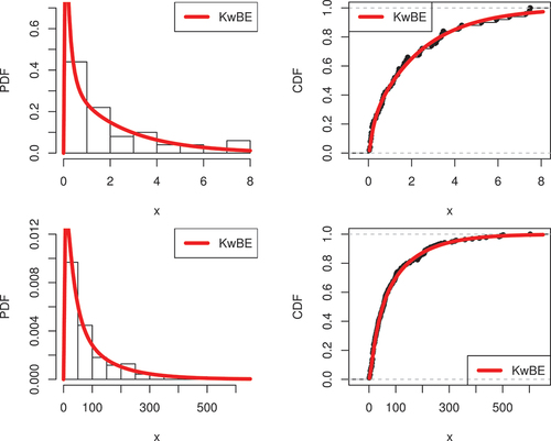
Table 5. The fitted models along with goodness-of-fit statistics, MLEs and S.E, first data

Model	-2$\hat{\mathrm{\ell }}$	$A^{\ast }$	$W^{\ast }$	KS	PV	Param.	Esti.	S.E
KwBE	81.02807	0.16211	0.01786	0.04531	1.000	$\hat{\theta }$	3.4481	0.1420
						$\hat{\varpi }$	1.5202	0.0738
						$\hat{a}$	4.4080	0.5467
						$\hat{b}$	0.1231	0.0169
KwPE	81.38482	0.18024	0.01945	0.05557	0.998	$\hat{\theta }$	3.7937	0.0517
						$\hat{\lambda }$	4.0342	0.0476
						$\hat{a}$	2.6302	0.0963
						$\hat{b}$	0.1135	0.0161
EE	83.37585	0.32787	0.03661	0.06695	0.979	$\hat{\alpha }$	0.4428	0.0867
						$\hat{\beta }$	0.8173	0.1462
MOE	83.22806	0.30430	0.03361	0.07476	0.943	$\hat{\alpha }$	0.3699	0.1262
						$\hat{a}$	0.5363	0.2806
EW	83.33341	0.30996	0.03409	0.06936	0.970	$\hat{\alpha }$	0.6359	0.7354
						$\hat{\beta }$	0.8410	0.4945
						$\hat{a}$	1.0785	1.0673
OWE	83.06346	0.33346	0.03721	0.05837	0.996	$\hat{\alpha }$	0.1029	0.1444
						$\hat{a}$	3.2647	4.8481
						$\hat{b}$	0.7906	0.1479
KE	83.89684	0.35807	0.04111	0.08956	0.817	$\hat{\alpha }$	3.9617	0.0607
						$\hat{a}$	0.8248	0.0488
						$\hat{b}$	0.1249	0.0178
BE	83.37565	0.32757	0.03657	0.06692	0.979	$\hat{\alpha }$	0.4098	1.9573
						$\hat{a}$	0.8178	0.1537
						$\hat{b}$	1.0773	4.9595
TLE	83.37585	0.32787	0.03661	0.06692	0.979	$\hat{\alpha }$	0.2214	0.0433
						$\hat{a}$	0.8172	0.1462
APEE	83.24683	0.30599	0.03347	0.06789	0.975	$\hat{\alpha }$	0.3978	0.1293
						$\hat{\gamma }$	0.5276	0.6801
						$\hat{\beta }$	0.8926	0.1971
TEE	83.29617	0.03444	0.31303	0.06753	0.977	$\hat{\alpha }$	0.4135	0.1203
						$\hat{\lambda }$	0.1942	0.4893
						$\hat{\beta }$	0.8606	0.1711
GEE	83.37542	0.32727	0.03652	0.06692	0.979	$\hat{\alpha }$	0.4377	0.1934
						$\hat{\beta }$	0.8473	1.0657
						$\hat{\lambda }$	0.9662	1.1465
EEP	83.24683	0.305995	0.03347	0.06788	0.975	$\hat{\alpha }$	0.3978	0.1293
						$\hat{\beta }$	0.8926	0.1972
						$\hat{\lambda }$	0.6388	1.2890
W	83.33635	0.31258	0.03442	0.06832	0.974	$\hat{\alpha }$	0.5812	0.1035
						$\hat{\beta }$	0.8792	0.0984
NH	83.48003	0.31746	0.03543	0.07885	0.915	$\hat{\alpha }$	0.9466	0.7005
						$\hat{\beta }$	0.5490	0.2112

Table 6. The fitted models along with goodness-of-fit statistics, MLEs and S.E, second data

Model	-2$\hat{\mathrm{\ell }}$	$A^{\ast }$	$W^{\ast }$	KS	PV	Param.	Esti.	S.E
KwBE	1031.748	0.16072	0.02027	0.03131	0.993	$\hat{\theta }$	0.0179	0.0082
						$\hat{\varpi }$	1.0624	0.2063
						$\hat{a}$	1.7971	0.4837
						$\hat{b}$	0.4429	0.1629
KwPE	1032.529	0.27743	0.03912	0.04150	0.903	$\hat{\theta }$	0.0124	0.0071
						$\hat{\lambda }$	2.2214	0.9222
						$\hat{a}$	1.3129	0.3032
						$\hat{b}$	0.6232	0.3235
EE	1037.75	1.20421	0.19422	0.07211	0.282	$\hat{\alpha }$	0.0102	0.0010
						$\hat{\beta }$	0.9109	0.0864
MOE	1034.747	0.55861	0.08571	0.05506	0.619	$\hat{\alpha }$	0.0077	0.0013
						$\hat{a}$	0.5225	0.1316
EW	1033.148	0.03638	0.27286	0.04499	0.841	$\hat{\alpha }$	0.2114	0.1612
						$\hat{\beta }$	0.5182	0.1170
						$\hat{a}$	3.2556	1.6762
OWE	1041.214	1.67031	0.27130	0.07734	0.211	$\hat{\alpha }$	0.0023	0.0002
						$\hat{a}$	2.9541	0.3688
						$\hat{b}$	0.7821	0.0429
KE	1037.775	1.20570	0.19447	0.07376	0.258	$\hat{\alpha }$	0.0108	0.0058
						$\hat{a}$	0.9150	0.0883
						$\hat{b}$	0.9519	0.4929
BE	1037.815	1.21304	0.19572	0.07389	0.256	$\hat{\alpha }$	0.0132	0.0083
						$\hat{a}$	0.9130	0.0892
						$\hat{b}$	0.7805	0.4811
TLE	1037.772	1.20787	0.19482	0.07050	0.308	$\hat{\alpha }$	0.0052	0.0005
						$\hat{a}$	0.9221	0.0865
APEE	1034.066	0.50873	0.07673	0.04981	0.739	$\hat{\alpha }$	0.0072	0.0014
						$\hat{\gamma }$	0.1422	0.1032
						$\hat{\beta }$	1.1146	0.0951
TEE	1035.506	0.79634	0.12540	0.05320	0.662	$\hat{\alpha }$	0.0084	0.0014
						$\hat{\lambda }$	0.4918	0.2173
						$\hat{\beta }$	1.0033	0.0875
GEE	1038.036	1.23954	0.20018	0.06815	0.347	$\hat{\alpha }$	0.0102	0.0014
						$\hat{\beta }$	0.7932	0.2346
						$\hat{\lambda }$	1.0877	0.2889
EEP	1034.06	0.50628	0.07629	0.04951	0.746	$\hat{\alpha }$	0.0071	0.0015
						$\hat{\beta }$	1.1147	0.0951
						$\hat{\lambda }$	1.9853	0.7620
W	1036.751	0.99738	0.15948	0.05707	0.573	$\hat{\alpha }$	0.0170	0.0043
						$\hat{\beta }$	0.9111	0.0485
NH	1034.997	0.58898	0.09054	0.05168	0.697	$\hat{\alpha }$	0.0208	0.0051
						$\hat{\beta }$	0.6931	0.0883

5.1. Comparative study of GASP based on the first data

Recently, Almarashi et al. (Almarashi et al., 2021) used the four-parameter exponential-based MOKw-E model to present the GASP in Table 7–8 using the same first data. The proposed KwBE model also has four parameters and extends the exponential model. Table 9 shows the comparative study of both models based on the first data set. The general findings of the analysis revealed that when $r=10$, $\beta =0.250$ and $a_1=1$, the proposed model is efficient, as shown by the fact that the design parameters ($g$ and $c$), as well as $n$ under the KwBE distribution, are the lowest when compared to the MOKw-E distribution.

Table 7. A GASP based on the KwBE model, $a=4.4080$, $b=0.1231$, $\varpi =1.5202$, first data

	$\mathit{r}\mathbf{=}\mathbf{5}$							$\mathit{r}\mathbf{=}\mathbf{10}$
		${\mathit{a}}_{\mathbf{1}}\mathbf{=}\mathbf{0.5}$			${\mathit{a}}_{\mathbf{1}}\mathbf{=}\mathbf{5}$			${\mathit{a}}_{\mathbf{1}}\mathbf{=}\mathbf{0.5}$			${\mathit{a}}_{\mathbf{1}}\mathbf{=}\mathbf{1}$
$\beta$	${\mathit{r}}_{\mathbf{2}}$	$\mathit{g}$	$\mathit{c}$	$\mathit{p}(a)$	$\mathit{g}$	$\mathit{c}$	$\mathit{p}(a)$	$\mathit{g}$	$\mathit{c}$	$p(a)$	$\mathit{g}$	$\mathit{c}$	$\mathit{p}(a)$
0.25	2	–	–	–	–	–	–	–	–	–	–	–	–
	4	27	3	0.9801	44	4	0.9778	6	4	0.983	2	2	0.9695
	6	6	2	0.9850	7	3	0.9827	2	2	0.9535	1	1	0.9778
	8	2	1	0.9704	3	2	0.9641	2	2	0.9874	1	0	0.9804
0.1	2	–	–	–	–	–	–	–	–	–	–	–	–
	4	44	3	0.9678	73	4	0.9635	9	4	0.9746	–	–	–
	6	9	2	0.9777	12	3	0.9706	2	2	0.9535	3	4	0.9669
	8	3	1	0.9560	4	2	0.9524	2	2	0.9874	2	3	0.9612
0.05	2	–	–	–	–	–	–	–	–	–	–	–	–
	4	57	3	0.9585	95	4	0.9527	11	4	0.9691	–	–	–
	6	12	2	0.9703	15	3	0.9634	5	3	0.9863	4	4	0.9562
	8	12	2	0.9927	15	3	0.9889	3	2	0.9812	2	3	0.9612
0.01	2	–	–	–	–	–	–	–	–	–	–	–	–
	4	934	4	0.9829	–	–	–	17	4	0.9526	–	–	–
	6	18	2	0.9558	146	4	0.9873	8	3	0.9782	10	5	0.9840
	8	18	2	0.9891	23	3	0.9830	4	2	0.975	5	4	0.9858

Remark: Hyphens (–) are inserted in required cells for a large sample size.

Table 8. A GASP under the KwBE model, $a=1.7971$, $b=0.4429$, $\varpi =1.0624$, second data

	$\mathit{r}\mathbf{=}\mathbf{5}$							$\mathit{r}\mathbf{=}\mathbf{10}$
		${\mathit{a}}_{\mathbf{1}}\mathbf{=}\mathbf{0.5}$			${\mathit{a}}_{\mathbf{1}}\mathbf{=}\mathbf{5}$			${\mathit{a}}_{\mathbf{1}}\mathbf{=}\mathbf{0.5}$			${\mathit{a}}_{\mathbf{1}}\mathbf{=}\mathbf{1}$
$\beta$	${\mathit{r}}_{\mathbf{2}}$	$\mathit{g}$	$\mathit{c}$	$\mathit{p}(a)$	$\mathit{g}$	$\mathit{c}$	$\mathit{p}(a)$	$\mathit{g}$	$\mathit{c}$	$p(a)$	$\mathit{g}$	$\mathit{c}$	$\mathit{p}(a)$
0.25	2	587	4	0.9623	–	–	–	30	5	0.9653	–	–	–
	4	8	2	0.9850	7	3	0.9862	2	2	0.9641	1	3	0.9546
	6	3	1	0.9704	3	2	0.9824	1	1	0.9598	1	3	0.9919
	8	3	1	0.9875	1	1	0.9690	1	1	0.9824	1	2	0.9819
0.1	2	–	–	–	–	–	–	–	–	–	–	–	–
	4	14	2	0.9739	12	3	0.9764	6	3	0.9885	3	4	0.9742
	6	4	1	0.9608	4	2	0.9767	3	2	0.9895	2	3	0.9839
	8	4	1	0.9834	4	2	0.9925	2	1	0.9651	1	2	0.9819
0.05	2	–	–	–	–	–	–	–	–	–	–	–	–
	4	18	2	0.9666	15	3	0.9706	8	3	0.9848	4	4	0.9657
	6	5	1	0.9512	5	2	0.9709	4	2	0.9861	2	3	0.9839
	8	5	1	0.9792	5	2	0.9906	2	1	0.9651	2	2	0.9641
0.01	2	–	–	–	–	–	–	–	–	–	–	–	–
	4	27	2	0.9503	23	3	0.9553	11	3	0.9791	5	4	0.9573
	6	27	2	0.9911	7	2	0.9595	5	2	0.9826	3	3	0.9760
	8	8	1	0.9670	7	2	0.9869	5	2	0.9951	2	2	0.9641

Remark: Hyphens (–) are inserted in required cells for a large sample size.

Table 9. Comparative study of GASP based on the KwBE and MOKw-E distribution, first data

	KwBE				MOKw-E
${\mathit{r}}_{\mathbf{2}}$	2	4	6	8	2	4	6	8
$n$	–	20	10	10	170	30	20	20
$g$	–	2	1	1	17	3	2	2
$c$	–	2	1	0	5	3	2	2
$p_{(a)}$	–	0.9695	0.9778	0.9804	0.9575	0.9813	0.9728	0.9882

5.2. Comparison of GASP and OSP

In this section, we analyzed the superiority of the GASP over the OSP by making a comparison of the sample sizes of the GASP with the OSP. A procedure termed lot sentencing uses ASP to decide whether arriving or departing batches should be admitted or denied based on a predetermined standard. The duration and sample size of the investigation are the two factors that professional investigators should consider most carefully, and both should be optimized. Although OSPs can help to attain this optimization, it is anticipated in this case that just a single item will be evaluated at a time. In contrast, a GASP may also accomplish the optimal cost and time when numerous objects can be evaluated in a tester by grouping the items. An upgrade of the OSP by taking $g=1$ when $n=r$ is the advocated GASP. Considering $g=1$ in $n=gr$, we analyzed the proposed GASP with the OSP. To accomplish this, we compared the recommended GASP for $r=5$ and $r=10$ with the OSP, when $g=1$ for the KwBE model with $a=1.7971$, $b=0.4429$, and $\varpi =1.0624$, for a given $\beta =\{0.25,0.1,0.05,0.01\}$ and $a_1=\{0.5,1\}$. Analysis of the sample sizes of the GASP and OSP from Table 10 indicated that GASP is the preferred approach when contrasted to OSP because GASP creates groups of objects and tests multiple items at once, whereas OSP determines a sufficiently large sample size and test single item at a time.

Table 10. Sample sizes of GASP and OSP, when $a=1.7971$, $b=0.4429$, $\varpi =1.0624$, second data

		$\mathit{r}\mathbf{=}\mathbf{5}$				$\mathit{r}\mathbf{=}\mathbf{10}$
		${\mathit{a}}_{\mathbf{1}}\mathbf{=}\mathbf{0.5}$		${\mathit{a}}_{\mathbf{1}}\mathbf{=}\mathbf{1}$		${\mathit{a}}_{\mathbf{1}}\mathbf{=}\mathbf{0.5}$		${\mathit{a}}_{\mathbf{1}}\mathbf{=}\mathbf{1}$
$\beta$	${\mathit{r}}_{\mathbf{2}}$	GASP	OSP	GASP	OSP	GASP	OSP	GASP	OSP
	4	40	40	35	35	20	23	10	12
0.25	6	15	18	15	15	10	13	10	12
	8	15	18	5	7	10	13	10	12
	4	70	73	60	63	60	63	30	30
0.1	6	20	23	20	20	30	30	20	22
	8	20	23	20	20	20	23	10	12
	4	90	93	75	281	80	80	40	40
0.05	6	25	27	25	27	40	42	20	22
	8	25	27	25	27	20	22	20	22
	4	135	137	115	117	110	112	50	50
0.01	6	135	137	35	37	50	50	30	32
	8	40	42	35	37	50	50	20	20

6. Concluding remarks

In this paper, we proposed a Kumaraswamy Bell exponential distribution holding the features of well-known Kumaraswamy and Bell numbers. Several commonly used properties of the KwBE distribution are presented such as the linear representation of the KwBE PDF, ordinary, moment-generating function using Wright generalized hyper-geometric function and Réyni entropy. Moreover, GASP for the truncated life test is presented using median life as a quality index. The essential design parameters are derived by defining the consumer risk and the test termination duration. The comparative study showed that GASP outperforms the OSP. The simulation-based empirical findings showed that maximum likelihood estimates are consistent and reliable under different sample size scenarios, revealing that the proposed model can be employed for border inferential analysis. The practical applicability of the proposed KwBE distribution is tested using two real data of quality control. Convincing results are obtained in comparison with several well-known extensions of the exponential distribution.

Disclosure statement

No potential conflict of interest was reported by the author(s).

Supplementary material

Supplemental data for this article can be accessed online at https://doi.org/10.1080/23311916.2023.2281062

1.

Appendix: Partial derivatives of the log-likelihood

$\begin{array}{rl}\frac{\mathrm{\partial }\mathrm{\ell }\left(\mathrm{\varnothing }\right)}{\mathrm{\partial }a}& =\frac{n}{a}+a\sum _{i=1}^{n}log\left[1-exp\left(-e^{\varpi }\left[1-e^{-\varpi \left(1-e^{-\theta t_i}\right)}\right]\right)\right]-nlog\left[1-exp\left(1-e^{\varpi }\right)\right]\\ & -\left(b-1\right)\sum _{i=1}^n\frac{{\left(\frac{1-exp\left(-e^{\varpi }\left[1-e^{-\varpi \left(1-e^{-\theta t_i}\right)}\right]\right)}{1-exp(1-e^{\varpi })}\right)}^{a}log\left(\frac{1-exp\left(-e^{\varpi }\left[1-e^{-\varpi \left(1-e^{-\theta t_i}\right)}\right]\right)}{1-exp(1-e^{\varpi })}\right)}{\left(1-{\left\{\frac{1-exp\left(-e^{\varpi }\left[1-e^{-\varpi \left(1-e^{-\theta t_i}\right)}\right]\right)}{1-exp(1-e^{\varpi })}\right\}}^a\right)},\\ \frac{\mathrm{\partial }\mathrm{\ell }\left(\mathrm{\varnothing }\right)}{\mathrm{\partial }b}& =\frac{n}{b}+b\sum _{i=1}^{n}log\left(1-{\left\{\frac{1-exp\left(-e^{\varpi }\left[1-e^{-\varpi \left(1-e^{-\theta t_i}\right)}\right]\right)}{1-exp(1-e^{\varpi })}\right\}}^a\right),\\ \frac{\mathrm{\partial }\mathrm{\ell }\left(\mathrm{\varnothing }\right)}{\mathrm{\partial }\varpi }& =\frac{n}{\varpi }+\sum _{i=1}^n\left[1-\left(1-e^{-\theta t_i}\right)\right]+\sum _{i=1}^n{e}^{\varpi }\left[e^{-\theta t_i-\varpi (1-e^{-\theta t_i})}-1\right]\end{array}$

$\begin{array}{rl}+\left(a-1\right)& \sum _{i=1}^n\frac{\left(\left(e^{-\theta t_i}-1\right){\mathrm{e}}^{\varpi -\left(1-e^{-\theta t_i}\right)\varpi }-e^{\varpi }\cdot \left(1-e^{-\varpi \left(1-e^{-\theta t_i}\right)}\right)\right)exp\left(-e^{\varpi }\left[1-e^{-\varpi \left(1-e^{-\theta t_i}\right)}\right]\right.}{exp\left(-e^{\varpi }\left[1-e^{-\varpi \left(1-e^{-\theta t_i}\right)}\right]\right)-1}\\ & -na\frac{e^{-e^{\varpi }+\varpi +1}}{1-exp(1-e^{\varpi })}+\left(b-1\right)\sum _{i=1}^n\frac{1}{\left(1-{\left\{\frac{1-exp\left(-e^{\varpi }\left[1-e^{-\varpi \left(1-e^{-\theta t_i}\right)}\right]\right)}{1-exp(1-e^{\varpi })}\right\}}^a\right)}\\ & \times \left(-a{\left\{\frac{1-exp\left(-e^{\varpi }\left[1-e^{-\varpi \left(1-e^{-\theta t_i}\right)}\right]\right)}{1-exp(1-e^{\varpi })}\right\}}^{a-1}\right)\\ & \times \frac{\left[e^{\varpi }\cdot \left(1-e^{-\varpi \left(1-e^{-\theta t_i}\right)}\right)-\left(e^{-\theta t_i}-1\right)e^{\varpi -\varpi \left(1-e^{-\theta t_i}\right)}\right]}{{\left(1-exp(1-e^{\varpi })\right)}^2}\left(1-exp(1-e^{\varpi })\right)\\ & \times exp\left(-e^{\varpi }\left[1-e^{-\varpi \left(1-e^{-\theta t_i}\right)}\right]\right)-\frac{e^{-e^{\varpi }+\varpi +1}\cdot \left(1-exp\left(-e^{\varpi }\left[1-e^{-\varpi \left(1-e^{-\theta t_i}\right)}\right]\right)\right)}{{\left(1-exp(1-e^{\varpi })\right)}^2},\\ & \frac{\mathrm{\partial }\mathrm{\ell }\left(\mathrm{\varnothing }\right)}{\mathrm{\partial }\theta }=\frac{n}{\theta }-\sum _{i=1}^n{t}_i-\varpi \sum _{i=1}^n{t}_i{e}^{-\theta t_i}-\varpi e^{\varpi }\sum _{i=1}^n{t}_i{e}^{-\theta t_i}\left(e^{-\varpi \left(1-e^{-\theta t_i}\right)}\right)\\ & +\left(a-1\right)\sum _{i=1}^n\frac{\varpi e^{-\theta t_i}{t}_i{e}^{-\varpi \left(1-e^{-\theta t_i}\right)}}{1-exp\left(-e^{\varpi }\left[1-e^{-\varpi \left(1-e^{-\theta t_i}\right)}\right]\right)}exp\left(-e^{\varpi }\left[1-e^{-\varpi \left(1-e^{-\theta t_i}\right)}\right]\right)\\ & +\left(b-1\right)\sum _{i=1}^n\frac{a{\left\{\frac{1-exp\left(-e^{\varpi }\left[1-e^{-\varpi \left(1-e^{-\theta t_i}\right)}\right]\right)}{1-exp(1-e^{\varpi })}\right\}}^{a-1}}{\left(1-{\left\{\frac{1-exp\left(-e^{\varpi }\left[1-e^{-\varpi \left(1-e^{-\theta t_i}\right)}\right]\right)}{1-exp(1-e^{\varpi })}\right\}}^a\right)}\\ & \times \left(\frac{exp\left(-e^{\varpi }\left[1-e^{-\varpi \left(1-e^{-\theta t_i}\right)}\right]\right)\left[e^{\varpi }{e}^{-\varpi \left(1-e^{-\theta t_i}\right)}\right]\left(t_i\varpi e^{-\theta t_i}\right)}{1-exp(1-e^{\varpi })}\right)\end{array}.$

The following GASP codes can be run for all Tables after changing

the respective parameters values.

g=seq(1,1000,1);c=c(0,1,2,3,4,5);lp2=double(length(g));

lp1=double(length(g));lp21=double(length(c)); lp22=double(length(c));

lp23=double(length(c));lp24=double(length(c));G1=double(length(c));

G2=double(length(c));G3=double(length(c));G4=double(length(c));

p=function(a,b,p,ratio,lambda,a1){

zeta=log(1-(1-((lambda)^(-1)*(log(log(1-(((1-(1-p)^(1/b))^(1/a))*(1-(exp(-exp(lambda)+1)))))+exp(lambda))))))

G=(1-exp((zeta*((ratio)^-1)*a1)))

y=(1-(1-((1-exp(-exp(lambda)*(1-exp(-lambda*G))))/(1-(exp(-exp(lambda)+1))))^(a))^(b))

return(y)

}

p2=round(p(1,1,0.5,c(2,4,6,8),1.25,0.5),4);p2;p1=round(p(1,1,0.5,1,1.25,0.5),4);p1

for(i in 1:length(c)){

for(j in 1:length(g)){

lp2[j]=(pbinom(c[i],5,p2[2]))^j ##changing the values in p2 from 1 to 4#

## for P2[1] you will not get any values but for p2[2] you will get values###

### see the tables in the paper and match the values ####

## and we need to change the value of a = 5or = 10###

lp1[j]=(pbinom(c[i],5,p1))^j

}

G1[i]=min(which(lp2 ≥ 0.95 & lp1 < 0.25));lp21[i]=round(lp2[G1[i]],4);

G2[i]=min(which(lp2 ≥ 0.95 & lp1 < 0.10));lp22[i]=round(lp2[G2[i]],4);

G3[i]=min(which(lp2 ≥ 0.95 & lp1 < 0.05));lp23[i]=round(lp2[G3[i]],4);

G4[i]=min(which(lp2 ≥ 0.95 & lp1 < 0.01));lp24[i]=round(lp2[G4[i]],4);

}

cbind(c,G1,lp21,G2,lp22,G3,lp23,G4,lp24)

References

- Afify, A. Z., Gemeay, A. M., & Ibrahim, N. A. (2020). The heavy-tailed exponential distribution: Risk measures, estimation, and application to actuarial data. Mathematics, 8(8), 1276. https://doi.org/10.3390/math8081276
- Al-Shomrani, A., Arif, O., Shawky, A., Hanif, S., & Shahbaz, M. Q. (2016). Topp-Leone family of distributions: Some properties and application. Pakistan Journal of Statistics & Operation Research, 12(3), 443–25. https://doi.org/10.18187/pjsor.v12i3.1458
- Alanzi, A. R., Imran, M., Tahir, M. H., Chesneau, C., Jamal, F., Shakoor, S., & Sami, W. (2023). Simulation analysis, properties and applications on a new Burr XII model based on the Bell-X functionalities. AIMS Mathematics, 8(3), 6970–7004. https://doi.org/10.3934/math.2023352
- Alexander, C., Cordeiro, G. M., Ortega, E. M., & Sarabia, J. M. (2012). Generalized beta-generated distributions. Computational Statistics & Data Analysis, 56(6), 1880–1897. https://doi.org/10.1016/j.csda.2011.11.015
- Algarni, A. (2022). Group acceptance sampling plan based on new compounded three-parameter Weibull model. Axioms, 11(9), 438. https://doi.org/10.3390/axioms11090438
- Almarashi, A. M., Khan, K., Chesneau, C., & Jamal, F. (2021). Group acceptance sampling plan using Marshall-Olkin Kumaraswamy exponential (MOKw-E) distribution. Processes, 9(6), 1066. https://doi.org/10.3390/pr9061066
- Ameeq, M., Tahir, M. H., Hassan, M. M., Jamal, F., Shafiq, S., & Mendy, J. T. (2023). A group acceptance sampling plan truncated life test for alpha power transformation inverted perks distribution based on quality control reliability. Cogent Engineering, 10(1), 2224137. https://doi.org/10.1080/23311916.2023.2224137
- Aslam, M., Balamurali, S., Jun, C. H., & Ahmad, M. (2013). Optimal design of skip lot group acceptance sampling plans for the Weibull distribution and the generalized exponential distribution. Quality Engineering, 25(3), 237–246. https://doi.org/10.1080/08982112.2013.769053
- Aslam, M., & Jun, C. H. (2009a). A group acceptance sampling plan for truncated life test having Weibull distribution. Journal of Applied Statistics, 36(9), 1021–1027. https://doi.org/10.1080/02664760802566788
- Aslam, M., & Jun, C. H. (2009b). A group acceptance sampling plans for truncated life tests based on the inverse Rayleigh and log-logistic distributions. Economic Quality Control, 25(2), 107–119. https://doi.org/10.1515/eqc.2010.008
- Aslam, M., Kundu, D., Jun, C. H., & Ahmad, M. (2011). Time truncated group acceptance sampling plans for generalized exponential distribution. Journal of Testing and Evaluation, 39(4), 671–677. https://doi.org/10.1520/JTE102921
- Aslam, M., Lio, Y., & Jun, C.-H. (2013). Repetitive acceptance sampling plans for burr type XII percentiles. The International Journal of Advanced Manufacturing Technology, 68(1–4), 495–507. https://doi.org/10.1007/s00170-013-4747-x
- Aslam, M., Mughal, A. R., Hanif, M., & Ahmad, M. (2010). Economic reliability group acceptance sampling based on truncated life tests using pareto distribution of the second kind. Communications for Statistical Applications and Methods, 17(5), 725–731. https://doi.org/10.5351/CKSS.2010.17.5.725
- Balakrishnan, N., Leiva, V., & Lopez, J. (2007). Acceptance sampling plans from truncated life tests based on the generalized Birnbaum-Saunders distribution. Communications in Statistics-Simulation and Computation, 36(3), 643–656. https://doi.org/10.1080/03610910701207819
- Bell, E. T. (1934). Exponential polynomials. The Annals of Mathematics, 35(2), 258–277. https://doi.org/10.2307/1968431
- Bourguignon, M., Silva, R. B., & Cordeiro, G. M. (2014). The Weibull-G family of probability distributions. Journal of Data Science, 12(1), 53–68. https://doi.org/10.6339/JDS.201401_12(1).0004
- Castellares, F., Ferrari, S. L., & Lemonte, A. J. (2018). On the bell distribution and its associated regression model for count data. Applied Mathematical Modelling, 56, 172–185. https://doi.org/10.1016/j.apm.2017.12.014
- Chakraborty, S., Handique, L., & Jamal, F. (2022). The kumaraswamy poisson-G family of distribution: Its properties and applications. Annals of Data Science, 9(2), 229–247. https://doi.org/10.1007/s40745-020-00262-4
- Cordeiro, G. M., & de Castro, M. (2011). A new family of generalized distributions. Journal of Statistical Computation and Simulation, 81(7), 883–898. https://doi.org/10.1080/00949650903530745
- Erdélyi, A. (Ed.). (1953). Higher transcendental functions. McGraw-Hill.
- Eugene, N., Lee, C., & Famoye, F. (2002). Beta-normal distribution and its applications. Communications in Statistics-Theory and Methods, 31(4), 497–512. https://doi.org/10.1081/STA-120003130
- Fayomi, A., Tahir, M. H., Algarni, A., Imran, M., Jamal, F., & Versaci, M. (2022). A new useful exponential model with applications to quality control and actuarial data. Computational Intelligence and Neuroscience, 2022, 1–27. https://doi.org/10.1155/2022/2489998
- Gupta, R. C., Gupta, P. L., & Gupta, R. D. (1998). Modeling failure time data by Lehman alternatives. Communications in Statistics-Theory and Methods, 27(4), 887–904. https://doi.org/10.1080/03610929808832134
- Hassan, M. M., Ameeq, M., Fatima, L., Naz, S., Sikandar, S. M., Kargbo, A., & Abbas, S. (2023). Assessing socio-ecological factors on caesarean section and vaginal delivery: An extended perspective among women of South-Punjab, Pakistan. Journal of Psychosomatic Obstetrics & Gynecology, 44(1), 2252983. https://doi.org/10.1080/0167482X.2023.2252983
- Hassan, M. M., Tahir, M. H., Ameeq, M., Jamal, F., Mendy, J. T., & Chesneau, C. (2023). Risk factors identification of COVID-19 patients with chronic obstructive pulmonary disease a retrospective study in Punjab Pakistan. Immunity Inflammation & Disease, 11(8), 981. https://doi.org/10.1002/iid3.981
- Jones, M. C. (2004). Families of distributions arising from distributions of order statistics. Test, 13(1), 1–43. https://doi.org/10.1007/BF02602999
- Khan, M. S., King, R., & Hudson, I. L. (2017). Transmuted Weibull distribution: Properties and estimation. Communications in Statistics-Theory and Methods, 46(11), 5394–5418. https://doi.org/10.1080/03610926.2015.1100744
- Khan, M. Z., Khan, M. F., Aslam, M., & Mughal, A. R. (2022). Fuzzy acceptance sampling plan for transmuted Weibull distribution. Complex & Intelligent Systems, 8(6), 4783–4795. https://doi.org/10.1007/s40747-022-00725-6
- Kumar, D., & Kumar, M. (2019). A new generalization of the extended exponential distribution with an application. Annals of Data Science, 6(3), 441–462. https://doi.org/10.1007/s40745-018-0181-0
- Liao, Q., Ahmad, Z., Mahmoudi, E., & Hamedani, G. G. (2020). A new flexible bathtub-shaped modification of the Weibull model: Properties and applications. Mathematical Problems in Engineering, 2020, 1–11. https://doi.org/10.1155/2020/3206257
- Marshall, A. W., & Olkin, I. (1997). A new method for adding a parameter to a family of distributions with application to the exponential and Weibull families. Biometrika, 84(3), 641–652. https://doi.org/10.1093/biomet/84.3.641
- Mudholkar, G. S., & Srivastava, D. K. (1993). Exponentiated Weibull family for analyzing bathtub failure-rate data. IEEE Transactions on Reliability, 42(2), 299–302. https://doi.org/10.1109/24.229504
- Muneeb Hassan, M., Ameeq, M., Jamal, F., Tahir, M. H., & Mendy, J. T. (2023). Prevalence of COVID-19 among patients with chronic obstructive pulmonary disease and tuberculosis. Annals of Medicine, 55(1), 285–291. https://doi.org/10.1080/07853890.2022.2160491
- Nadarajah, S. (2011). The exponentiated exponential distribution: A survey. AStA Advances in Statistical Analysis, 95(3), 219–251. https://doi.org/10.1007/s10182-011-0154-5
- Nadarajah, S., Cordeiro, G. M., & Ortega, E. M. (2012). General results for the Kumaraswamy-G distribution. Journal of Statistical Computation and Simulation, 82(7), 951–979. https://doi.org/10.1080/00949655.2011.562504
- Nadarajah, S., & Haghighi, F. (2011). An extension of the exponential distribution. Statistics, 45(6), 543–558. https://doi.org/10.1080/02331881003678678
- Naz, S., Al-Essa, L. A., Bakouch, H. S., & Chesneau, C. (2023). A transmuted modified power-generated family of distributions with practice on submodels in insurance and reliability. Symmetry, 15(7), 1458. https://doi.org/10.3390/sym15071458
- Naz, S., Tahir, M. H., Jamal, F., Ameeq, M., Shafiq, S., & Mendy, J. T. (2023). A group acceptance sampling plan based on flexible new Kumaraswamy exponential distribution: An application to quality control reliability. Cogent Engineering, 10(2), 2257945. https://doi.org/10.1080/23311916.2023.2257945
- Pogány, T. K. (2015). The exponentiated exponential Poisson distribution revisited. Statistics, 49(4), 918–929. https://doi.org/10.1080/02331888.2014.932794
- Rao, G. S. (2009). A group acceptance sampling plans based on truncated life tests for Marshall-Olkin extended Lomax distribution. Electronic Journal of Applied Statistical Analysis, 3(1), 18–27. https://doi.org/10.1285/i20705948v3n1p18
- Ristić, M. M., & Balakrishnan, N. (2012). The gamma-exponentiated exponential distribution. Journal of Statistical Computation and Simulation, 82(8), 1191–1206. https://doi.org/10.1080/00949655.2011.574633
- Tahir, M. H., & Cordeiro, G. M. (2016). Compounding of distributions: A survey and new generalized classes. Journal of Statistical Distributions and Applications, 3(1), 1–35. https://doi.org/10.1186/s40488-016-0052-1
- Tahir, M. H., & Nadarajah, S. (2015). Parameter induction in continuous univariate distributions: Well-established G families. Anais da Academia Brasileira de Ciencias, 87(2), 539–568. https://doi.org/10.1590/0001-3765201520140299
- Tsai, T. R., & Wu, S. J. (2006). Acceptance sampling based on truncated life tests for generalized Rayleigh distribution. Journal of Applied Statistics, 33(6), 595–600. https://doi.org/10.1080/02664760600679700
- Weibull, W. (1951). A statistical distribution function of wide applicability. Journal of Applied Mechanics, 18(3), 293–297. https://doi.org/10.1115/1.4010337