Automated histopathological detection and classification of lung cancer with an image pre-processing pipeline and spatial attention with deep neural networks

Abstract

Lung Cancer is a major cancer in the world and specifically India. Histopathological examination of tumorous tissue biopsy is the gold standard method used to clinically identify the type, sub-type, and stage of cancer. Two of the most prevalent forms of lung cancer: Adenocarcinoma & Squamous Cell Carcinoma account for nearly 80% of all lung cancer cases, which makes classifying the two subtypes of high importance. Proposed in this study is a data pre-processing pipeline for the H&E-stained lung biopsy images along with a customized EfficientNetB3-based Convolutional Neural Network employing spatial attention, trained on a public three-class lung cancer histopathological image dataset. The pre-processing pipeline employed before training, validation and testing helps enhance features of the histopathological images and removes biases due to stain variations for increased model robustness. The usage of a pre-trained CNN helps the deep learning model generalize better with the pre-trained weights, while the attention mechanism On three-fold validation, the classifier bagged accuracies of 0.9943 ± 0.0012 and 0.9947 ± 0.0018 and combined F1-Scores of 0.9942 ± 0.0042 and 0.9833 ± 0.0216 over the validation and testing data respectively. The high performance of the model combined with its computational efficiency could enable easy deployment of our model without necessitating infrastructure overhaul.

Keywords:

• Adenocarcinoma
• convolutional neural network EfficientNetB3
• histopathological images
• lung cancer
• squamous cell carcinoma

REVIEWING EDITOR:

• Jin Zhongmin, Southwest Jiaotong University, China

SUBJECTS:

• Biomedical Engineering
• Artificial Intelligence
• Computation

1. Introduction

Lung cancer is one of the most frequent and lethal tumors in the world, accounting for 11.4% of new cancer cases and 18.4% of cancer deaths in 2020 (Sung et al., 2021). Lung cancer accounts for 5.9% of all cancers and 8.1% of cancer-related deaths in India (Singh et al., 2021). The anticipated number of new lung cancer cases in India in 2013 was 90,000, and this figure is expected to rise to more than 1 lakh in the following five years (Times of India, n.d). Lung cancer is more common in men (about 70% of cases), however the prevalence of lung cancer in women has slowly increased over the last decade (D, 2022).

Tobacco smoking is the most significant contributor to the rise in lung cancer cases in India, accounting for around 80% of all cases (Singh et al., 2021). With an estimated 267 million tobacco smokers, India is the world’s second largest consumer and third largest producer of tobacco (Cancer Statistics - India Against Cancer, n.d). Tobacco-related malignancies account for 27% of all cancers in both sexes combined, however this varies greatly across the country (Report of National Cancer Registry Programme 2020, 2021d). Tobacco, however, is not the only cause of lung cancer. Other variables that may contribute to the development of lung cancer include air pollution, occupational exposure, genetic predisposition, and infections (Subramanian & Govindan, 2007). Air pollution is a serious environmental health problem in India, particularly in metropolitan areas where particulate matter (PM2.5 and PM10) levels exceed WHO limits by many orders of magnitude (Air Pollution, n.d). By generating inflammation, oxidative stress, and DNA damage, these pollutants can raise the risk of lung cancer (Loomis et al., 2014). Occupational exposure to asbestos, radon, arsenic, chromium, nickel, and other carcinogens has also been linked to an increased risk of lung cancer in some industries (Alberg & Samet, 2003). In some cases of lung cancer, genetic susceptibility may play a role, particularly in nonsmokers or those with a family history of lung cancer (Pao & Girard, 2011). Tuberculosis, human papillomavirus (HPV), and Epstein-Barr virus (EBV) infections may also be linked to lung cancer by generating chronic inflammation or changing cellular pathways (Syrjänen, 2002).

Lung cancer diagnosis and treatment in India encounter various problems, including a lack of awareness, late presentation, a lack of screening and diagnostic facilities, a high treatment cost, and limited access to health care (Noronha et al., 2012). Cough, chest pain, shortness of breath, and weight loss are all indications of lung cancer (Cooley, 2000). When people seek medical attention, their lung cancer is frequently advanced, reducing their odds of survival. Lung cancer survival in India is predicted to be around 12%, compared to 19% globally (Bray et al., 2018).

Lung squamous cell carcinoma and lung adenocarcinoma are two types of non-small cell lung cancer (NSCLC), which account for about 80% of all lung cancers. They have different characteristics, risk factors, molecular features, and treatments. Originating in the bronchi, Lung Squamous Cell Carcinoma (L-L-SCC) is distinguished by tumour cells with a squamous appearance, like skin cells. Tobacco use is more closely linked to lung squamous cell carcinoma than to any other type of NSCLC. It frequently metastasizes to locoregional lymph nodes early in its course but disseminates outside the thorax later than other kinds of lung cancer (Kawase et al., 2011). The second sub-type, Lung Adenocarcinoma (L-A) develops in the alveoli, which are small air sacs that assist the lungs exchange oxygen and carbon dioxide. Tumour cells produce glands or secrete mucus, which distinguishes it. The most frequent type of lung cancer is lung adenocarcinoma, which is more common in younger women and Asia. It is also the most frequent type of lung cancer in nonsmokers, even though smoking remains a substantial risk factor. It grows more slowly and spreads farther than other types of lung cancer (Wang et al., 2020).

Histopathology is the part of pathology that involves the microscopic inspection of tissues and cells, is vital in the diagnosis of various disorders, including cancer and identifying the kind and stage of cancer. Pathologists use manual histopathological detection of cancer to take tissue samples from biopsies and microscopically assess the size, shape, and arrangement of the cells, as well as aspects of the surrounding tissue. These samples are then prepared for inspection by fixation, embedding, and other types of staining, with chemicals such as haematoxylin and eosin, that highlight cellular properties such as nucleic acids, allowing for the detection of malignant cells and the assessment of their characteristics (Goldblum et al., 2017). In the manual histological diagnosis of the two major forms of lung cancer, L-A is distinguished by glandular differentiation, whereas L-SSC is distinguished by keratinization and intercellular bridges (Kumar et al., 2018).

Cancer detection and diagnosis utilising histopathological examination rely on pathologists’ subjective interpretation, many factors such as sample quality and human error may result in incorrect diagnosis (Jahn et al., 2020). Several research have been undertaken to assist pathologists in detecting tumours using machine learning-based classifiers built and validated using histopathology pictures (Van der Laak et al., 2021). Convolutional neural networks (CNNs) are artificial neural networks that can learn to recognise patterns and features and are useful in a wide range of clinical and non-clinical applications. These neural networks can be trained to identify and extract key aspects from picture data, such as textures, colours, and forms, to classify the images (O'Shea & Nash, 2015).

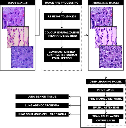
This paper describes a study entailing a three-class lung cancer dataset of histopathology images that was pre-processed for colour normalisation and feature enhancement. These processed images were then utilised to train and validate a customized deep convolutional neural network. This CNN incorporates transfer learning on a pre-trained neural network, as well as additional trainable layers to fine-tune the network to the ternary dataset. Additionally, a spatial attention mechanism is also included, enabling the neural network to focus on certain areas of the histopathological images by assigning different levels of relevance to distinct regions of the input. Figure 1 graphically represents the workflow of the proposed model.

Figure 1. Intended implementation workflow for the proposed model.

As shown in Table 1, several studies have been conducted on the publicly available LC25000 dataset. In (Liu et al., 2022) augmentation techniques, including flip and noise overlay were applied to the dataset before being trained on a custom CNN SENet50_CroReLU, yielding an impressive accuracy of 98.33%, with high precision and sensitivity scores of 98.38% and 98.35%, respectively (Hatuwal & Thapa, 2020). employed a custom CNN without any pre-processing, achieving a notable accuracy of 97.2%, with balanced F1-score, precision, and sensitivity all reported at 97.33% across the tree classes. Similarly (Mangal et al., 2020), also employed a custom CNN and reported a slightly higher accuracy of 97.89%.

Table 1. Pre-processing & deep learning approaches and reported performance evaluation of existing work.

Ref. no	Pre-Processing	Model	Validation Accuracy	Average F1-score	Average Precision	Average Sensitivity
(Liu et al., 2022)	Flipping, noise overlay	Custom CNN	0.9833	Not Reported	0.9838	0.9835
(Hatuwal & Thapa, 2020)	None	Custom CNN	0.972	0.9733	0.9733	0.9733
(Mangal et al., 2020)	None	Custom CNN	0.9789	Not Reported	Not Reported	Not Reported
(Civit-Masot et al., 2022)	Compression, Colour normalization	Custom CNN	0.9711	0.9713	0.9716	0.9713
(Civit-Masot et al., 2022)	Compression, converting to greyscale	Custom CNN	0.9401	0.9403	0.9403	0.9403
(Phankokkruad, 2021)	Resizing	Ensemble CNN	0.91	0.91	0.92	0.91
(Pradhan et al., 2022)	Colour normalization, Segmentation	AlexNet for feature extraction, Random Forest for classification	0.985	Not Reported	Not Reported	0.9798

Civit-Masot et al. (2022) investigated two different pre-processing methods within the same paper and trained their custom CNN model across varying number of epochs. Pre-processing the images using compression and colour normalization performed best when trained for 50 epochs leading to an accuracy of 97.11% and an average F1-score, precision, and sensitivity of 97.13% across the three classes. While the addition of grayscale conversion alongside compression resulted in an accuracy of 94.01%, with consistent F1-score, precision, and sensitivity values of 94.03% across the three classes (Phankokkruad, 2021) resized the images before using them to train on an ensemble CNN architecture achieving an accuracy of 91% with corresponding F1-score and sensitivity values of 91%, and precision slightly higher at 92%. Lastly (Pradhan et al., 2022), combined colour normalization and segmentation techniques with an AlexNet for feature extraction and a Random Forest classifier, yielding an accuracy of 98.5% and a sensitivity score of 97.98%.

A fundamental objective of the work described here is to explore the usage of novel deep learning techniques such as attention mechanisms and regularization techniques together with traditional techniques such as transfer learning, something not explored widely in previous works in the field. Additionally, employing a comprehensive pre-processing pipeline for removing biases while enhancing features has also been explored, in contrast to previous works that explore only one or few elements of the pipeline separately.

The objectives of the undertaken study include:

• Using a widely used histopathological dataset of lung tumour tissue samples to train, validate and test a classifier.

• Perform feature enhancement with image processing techniques to help better the training process extract features.

• Color normalization of histopathology images is crucial for training deep learning networks, ensuring consistent and reliable model performance across diverse datasets

• Making use of spatial attention mechanisms to enabling selective focus on specific regions within an image, enhancing feature extraction for better classification accuracy

• Training the network individually thrice with a different training and validation split to avoid any training biases.

2. Materials and methods

As illustrated in Figure 2, the experimental workflow for the study described in this paper started off with obtaining the dataset and then pre-processing it. These processed images have then been used to train, validate, and test the neural network which then classifies the given input across the three classes.

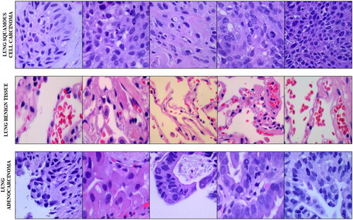
Figure 2. Sample images from the LC25000 lung-cancer data subset.

2.1. Dataset

Collected by researchers in Tampa, Florida, USA, the LC25000 dataset is a five-class histopathological image dataset containing a binary colon cancer data sub-set and a ternary class lung cancer data sub-set that has been used in this study. The three class lung cancer data sub-set started off with 250 images across the three classes: Lung Benign Tissue, Lung Adenocarcinoma and Lung Squamous Cell Carcinoma. These 750 images have then been cropped from their original 1024x768 resolution to 768x768 resolution to maintain a 1:1 aspect ratio before augmentation. The augmentation pipeline included left and right rotations (up to 25 degrees, 100% probability) and by horizontal and vertical flips (50% probability). This brought it to 5000 images per class, and 15000 images across all classes of the lung cancer sub-set. 5 sample images from the lung-subset of the LC25000 dataset has been shown in Figure 2.

For our model, the lung cancer data-subset has been further split into training (75%), validation, (15%) and testing (10%). Across the three-fold validation, the images across the training and the validation splits were dynamically interchanged, while the test set remained constant. All three classes in the dataset had 3750 images for training, 750 images for validation and 500 images for testing individually.

2.2. Data pre-processing pipeline

Before using the lung sub-set of the LC25000 dataset, histopathological images have been pre-processed to normalize their colours, enhance contrast, sharpen the images, and finally reduce their size. This pipeline builds on pre-processing pipeline as demonstrated in (Nayak et al., 2023). As described in Figure 3, the pre-processing pipeline for the dataset starts off with Colour Normalization, which has been carried out in this study using Reinhard’s colour normalization method. Colour normalization techniques are predominantly used in histopathological analysis to remove non-uniformities in colours caused by staining inconsistencies. This normalization technique, commonly used in histopathology, matches the colour distribution of the entire dataset to one selected reference image by using a linear transform in the Lαβ colour space. In this colour space, the mean and standard deviations are calculated for α (red and green) and β (blue and yellow) for the target and references images.

Figure 3. Image data pre-processing pipeline. Note: Resized images not reduced to scale.

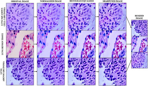
A linear transformation is used to align the colour distribution of the dataset image to a target image, which is generated using a histogram matching approach that minimises the difference between two distributions. The Gaussian distributions are used to estimate the colour distributions of the dataset and reference images, and the linear transformation is represented by the global colour transfer function. The standard deviation and mean deviation in the reference and dataset for each channel: α (red and green) and β (blue and yellow) are used to normalise the image’s colour distribution.

The next pre-processing technique in the pipeline is Contrast Limited Adaptive Histogram Equalization (CLAHE). This technique enhances contrast by working on regions/tiles of the image. The contrast of each tile is enhanced with the target of having the histogram of the entire output region approximately matching the histogram specified by the distribution. Using bilinear interpolation artificial boundaries are removed and adjacent tiles are combined back to form the full image. Using CLAHE over traditional histogram equalization helps curb the overamplification of noise in homogenous regions in the output image by enhancing local contrast and limiting noise amplification using a pre-defined clip limit to clip the histogram at a given value. Values exceeding the clip limit are then redistributed among other areas in the histogram.

Following CLAHE, Unsharp Masking is used to sharpen the image with the objective of enhancing fine detail in the image. By accentuating high-frequency components, unsharp masking can effectively improve image contrast and visual clarity, making it a popular method for enhancing the sharpness of digital images in various applications, from photography to medical imaging. It is accomplished by subtracting a blurred version of the image from the original image, followed by computing, and adding a scaled down version of the original image. The final image has sharper edges and higher contrast.

The normalized, histogram equalized and sharpened images have then been Resized using the nearest neighbour method from 768x768 resolution to 224x224 to reduce the computation complexity of the images during the training and validation of the neural network with the dataset. This method involves assigning each pixel in the resized image the value of its nearest neighbour in the original image.

2.3. Transfer learning and spatial attention

As depicted in Figure 4, a custom convolutional neural network employing transfer learning using a pre-trained neural network functional unit with spatial attention and trainable layers has been fine-tuned on the lung cancer data subset.

Figure 4. Model architecture of EfficientNetB3 with trainable layers and spatial attention block used in this study. Layers in the blue box indicate the non-trainable blocks.

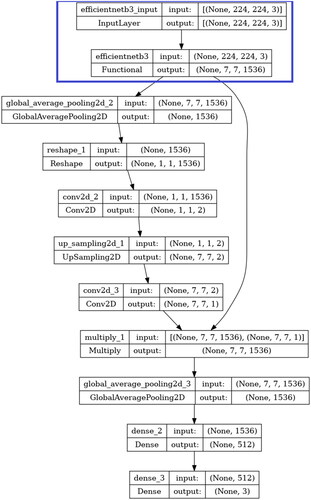
The pre-trained network used for transfer learning is EfficientNetB3. EfficientNetB3 belongs to a series of convolutional neural networks known as EfficientNet, which was introduced in 2019 by Tan and Le (Tan & Le, 2019). The main idea behind EfficientNet’s development is the recognition that simply scaling up individual aspects of a neural network, such as its depth, width, or resolution, can become inefficient and costly in terms of computational resources. To overcome this challenge, the researchers proposed a novel approach called compound scaling, by uniformly scaling all dimensions of the network. This method ensures that the network’s capacity grows efficiently across multiple dimensions, resulting in improved performance without a significant increase in computational demands. The scaling is controlled by a single parameter, referred to as phi (φ). EfficientNetB3 has a scaling coefficient of 3. Despite being larger, it maintains efficiency in terms of both model size and computational resources. This efficiency is achieved using specialized architectural components, such as mobile inverted bottleneck convolutional blocks and squeeze-and-excitation blocks, as well as efficient feature aggregation techniques.

The pre-trained network used for transfer learning is EfficientNetB3. EfficientNetB3 belongs to a series of convolutional neural networks known as EfficientNet, which was introduced in 2019 by Tan and Le (Tan & Le, 2019). The main idea behind EfficientNet’s development is the recognition that simply scaling up individual aspects of a neural network, such as its depth, width, or resolution, can become inefficient and costly in terms of computational resources. To overcome this challenge, Tan and Le proposed a novel approach called compound scaling, which involves uniformly scaling all dimensions of the network. This method ensures that the network’s capacity grows efficiently across multiple dimensions, resulting in improved performance without a significant increase in computational demands. The scaling is controlled by a single parameter, referred to as phi (φ). EfficientNetB3, specifically, has a scaling coefficient of 3, indicating its larger size compared to the base EfficientNet model. Despite being larger, EfficientNetB3 maintains efficiency in terms of both model size and computational resources. This efficiency is achieved using specialized architectural components, such as mobile inverted bottleneck convolutional blocks and squeeze-and-excitation blocks, as well as efficient feature aggregation techniques.

The pre-trained network used for transfer learning is EfficientNetB3. EfficientNetB3 belongs to a series of convolutional neural networks known as EfficientNet, which was introduced in 2019 by Tan and Le. The main idea behind EfficientNet’s development is the recognition that simply scaling up individual aspects of a neural network, such as its depth, width, or resolution, can become inefficient and costly in terms of computational resources. To overcome this challenge, Tan and Le proposed a novel approach called compound scaling, which involves uniformly scaling all dimensions of the network. This method ensures that the network’s capacity grows efficiently across multiple dimensions, resulting in improved performance without a significant increase in computational demands. The scaling is controlled by a single parameter, referred to as phi (φ). EfficientNetB3, specifically, has a scaling coefficient of 3, indicating its larger size compared to the base EfficientNet model. Despite being larger, EfficientNetB3 maintains efficiency in terms of both model size and computational resources. This efficiency is achieved using specialized architectural components, such as mobile inverted bottleneck convolutional blocks and squeeze-and-excitation blocks, as well as efficient feature aggregation techniques.

The pre-trained network used for transfer learning is EfficientNetB3. EfficientNetB3 belongs to a series of convolutional neural networks known as EfficientNet, which was introduced in 2019 by Tan and Le. The main idea behind EfficientNet’s development is the recognition that simply scaling up individual aspects of a neural network, such as its depth, width, or resolution, can become inefficient and costly in terms of computational resources. To overcome this challenge, Tan and Le proposed a novel approach called compound scaling, which involves uniformly scaling all dimensions of the network. This method ensures that the network’s capacity grows efficiently across multiple dimensions, resulting in improved performance without a significant increase in computational demands. The scaling is controlled by a single parameter, referred to as phi (φ). EfficientNetB3, specifically, has a scaling coefficient of 3, indicating its larger size compared to the base EfficientNet model. Despite being larger, EfficientNetB3 maintains efficiency in terms of both model size and computational resources. This efficiency is achieved through the use of specialized architectural components, such as mobile inverted bottleneck convolutional blocks and squeeze-and-excitation blocks, as well as efficient feature aggregation techniques.

Used in this study the base EfficientNetB3 is pre-trained with its weights set to the 1000 class ImageNet database, with an overall functional size of 48MB, having 12.3 million parameters across 210 layers. On Keras, it has Top-1 & Top-5 Accuracies of 81.6% and 95.7%, which is higher than that of mainstream networks such as ResNet50 and InceptionV3, both coming in at 74.9% & 92.1% and 77.9% & 93.7%, while being almost twice as large at 98MB & 92MB, respectively.

EffecientNet has been widely used for medical disease detection (Huri et al., 2022) employed transfer learning on an EfficientNet model to classify brain tumours from MRI images, yielding a 98% accuracy. Similarly, in (Batool & Byun, 2023) the authors developed an EfficientNet-based model to classify leukaemia from white blood cell images, achieving an accuracy exceeding 99%.

The EfficientNetB3 used in this study for transfer learning has its weights set and locked to those of its pre-training on the ImageNet database, with further training during fine-tuning disabled. Instead, the attention mechanism and trainable layers learn features from the processed ternary lung cancer histopathological image dataset during the fine-tuning training. The first block after the EfficientNetB3 functional unit is the spatial attention layers. The spatial attention mechanism allows the model to focus on specific parts of the input by assigning different levels of importance to different spatial locations. Here, the attention mechanism computes an attention tensor which signifies the importance of each spatial location in the output of the EfficientNetB3 unit. This tensor scales the output of EfficientNetB3 (ENB3) unit, enabling it to focus on specific parts of the image when classifying.

This attention tensor is first computed by adding a global average pooling layer to the dense layer of the ENB3 unit to reduce the spatial dimensions of the tensor to 1x1 without reducing the number of channels. This is then reshaped to (1,1,-1) with the -1 signifying the size of this dimension being inferred from the size of the input tensor. After this, a 1x1 Convolutional Layer with a sigmoid activation and 2 filters is applied to the reshaped tensor to produce a resultant tensor of shape (1,1,2), with the two channels representing the attention values for each class. This attention tensor is then upsampled to be match the spatial dimensions of the ENB3 unit with a UpSample2D layer that it then succeeded by a 1x1 convolutional layer with sigmoid activation and 1 filter which gives a resultant tensor having shape (224,224,1) that is identical to those of the spatial dimensions of the ENB3 model. This upsampled attention tensor then undergoes element-wise multiplication with the output of the ENB3 model that scales each spatial location in the output of the ENB3 unit with its corresponding attention value. This enables the neural network to focus on specific parts of the image, while making its prediction for classification. The attention block is then followed by the trainable layers featuring another global average pooling layer which is then followed by a dense layer having 512 neurons and ReLU activation and a final dense layer having 3 neurons, corresponding to the number of classes, and SoftMax activation.

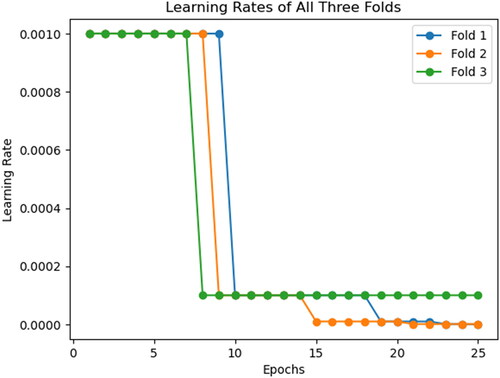
Two additional callbacks have been employed during the training of the convolutional neural network: Learn Rate Decay on Plateau and Early Stopping. Learn rate decay on plateauing has been implemented using the ReduceLRonPlateau callback, that reduces the learn rate by a set value of 0.1 if the validation loss does not improve over two epochs. Similarly, Early Stopping is also implemented using its namesake callback to stop the training of the neural network should the validation loss not decrease over three epochs. Should the training be stopped by this callback, it will restore the weights attained by the model when it achieved the lowest validation loss. As shown in Figure 5, we can notice the learn rate for the three folds initially reduce between the seventh and ninth epochs, and Fold 2 stopping early on the twenty-third epoch. The rationale for having these callbacks monitor the validation loss is due to the metric shedding light on the CNN’s ability to generalize to new and unseen data. Should this metric stabilize or begin increasing, it indicates that overfitting has started in the training process. An additional advantage of employing learn rate decay on plateau is that it enables the model to make large updates with the larger learn rate during initial epochs of training, with the CNN quickly reaching the neighbourhood of the optimal weights. These large updates can then be made smaller and more precise to avoid overshooting the optimal solution. Similarly, this technique also helps the model escape the local minima by dropping its learn rate, if the CNN gets stuck during the training process.

Figure 5. Learn rate decay history over all three folds.

2.4. Experimental setup

The pre-processing of the images in the dataset has been done on MathWorks MATLAB 2022b, making use of the Image Batch Processor from the Image Processing Toolbox. Deep learning trials have been performed using the Keras on TensorFlow on Kaggle Code platform. The execution environment for MATLAB was the single CPU while that for Kaggle Code was the Nvidia P100 GPU with 16GB VRAM. Multiple trials featuring varying hyperparameters such as the maximum number of epochs, initial learn rate, optimizer, loss function and batch size have been used, with the hyperparameters of the top performing trials across the three folds tabulated in Table 2.

Table 2. Experimental hyper-parameters for deep learning trials.

Parameter	Value
Maximum Epochs	15 20 25 30
Batch Size	32 64 128 256
Initial Learn Rate	0.1 0.001 0.0001
Minimum Learn Rate	1e-6 1e-7 1e-8 1e-9 1e-10
Learn Rate Decay Factor	0.01 0.05 0.1 0.5
Optimization Algorithm	SGDM ADAM RMSPROP
Loss Function	Categorical Cross-Entropy
ReduceLRonPlateau Patience	1 2 3 4 5 6
Early Stopping Patience	1 2 3 4 5 6
Callbacks Monitor	Training Loss Validation Loss Training Accuracy Validation Accuracy
Restore Best Weights on Early Stopping	True False

Bold indicates final selected parameters.

As represented in the table, multiple trials showed the network best performing when using the Adaptive Moment Estimation (ADAM) optimization algorithm, with loss function Categorical Cross-Entropy due to its multi class nature. The neural networks were trained for a maximum of 25 epochs, with an initial and maximum learn rate values of 0.001 and 1e-08 respectively. The callbacks for Early Stopping and Learn Rate Decay were both set to monitor the Validation Loss and having patience of 3 and 2 epochs respectively. The Early Stopping also included the condition to restore the weights of the best performing epoch (lowest validation loss) should the training be halted early. The training, validation, and testing data splits each had a batch size of 128, as 256 and above exhausted the available resources.

To ensure that the trained and validated model is not biased to any one split of the training and validation data, the deep learning trials have been conducted thrice with the same parameters and data, but with randomized training and validation data split that changed across each trial. This was done to observe reproducibility of the results with varying data split. Hence, all reported metrics will be represented with a mean and standard deviation values.

3. Results

Detailed in this section are the accuracies and losses obtained for the training and validation data subsets, along with the test accuracy, all obtained from their respective confusion matrices as shown in Figure 6.

Figure 6. Accuracy and loss plots for the training and validation data subsets over the 25-epoch training. Fold 0 (Left), Fold 1 (Centre) and Fold 2 (Right).

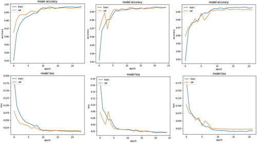
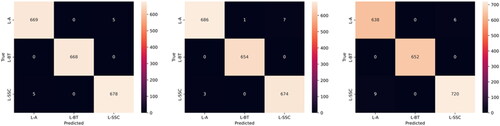
From these confusion matrices, that have been generated alongside the training and validation plots of accuracy and loss, represented in Figure 7, over the training-validation period, the class-specific performance evaluation metrics such as precision, recall and F1-Score have also been calculated and reported.

Figure 7. Confusion matrices for the validation data across Fold 0 (Left), Fold 1 (Centre) and Fold 2 (Right).

3.1. Experimental results and calculated metrics – validation data

Table 3 highlights the performance of the proposed model during training and validation across the three folds. The metrics include Training Accuracy, Training Loss, Validation Accuracy, and Validation Loss.

Table 3. Experimental accuracy & loss over training & validation data.

Fold	Training Accuracy	Training Loss	Validation Accuracy	Validation Loss
0	0.9972	0.0104	0.9956	0.0144
1	0.9951	0.0158	0.9946	0.0167
2	0.9953	0.0163	0.9926	0.0233
Mean ± SD	0.9959 ± 0.0009	0.0124 ± 0.0027	0.9943 ± 0.0012	0.0181 ± 0.0037

We can calculate the accuracy, precision, recall, specificity and F1 score from the values obtained from the confusion matrices in Figure 8, represented in Table 3. In the first fold, the model achieved a high Training Accuracy of 0.9972, the corresponding Training Loss was 0.0104. For validation, the model attained a Validation Accuracy of 0.9956, and a Validation Loss of 0.0144. In the second fold, the model achieved a Training Accuracy of 0.9951 and a Training Loss of 0.0158. The Validation Accuracy remained high at 0.9946. The Validation Loss was 0.0167. In the third fold, the model continued to exhibit robustness with a Training Accuracy of 0.9953 and a Training Loss of 0.0163. The Validation Accuracy remained high at 0.9926 with a Validation Loss of 0.0233.

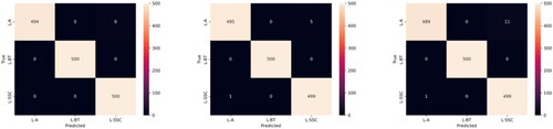
Figure 8. Confusion matrices for the testing data across Fold 0 (Left), Fold 1 (Centre) and Fold 2 (Right).

Across all three cross-validation folds, the model demonstrated consistent performance. The mean values for Training Accuracy, Training Loss, Validation Accuracy, and Validation Loss were 0.9959, 0.0124, 0.9943, and 0.0181, respectively. The standard deviations (SD) for these metrics were 0.0009, 0.0027, 0.0012, and 0.0037, respectively.

Tables 4 and 5 provide a comprehensive overview of the metrics obtained from the validation dataset, including sensitivity, specificity, precision, accuracy, and F1-score. For the ‘L-SCC’ class, the model achieved Precision values of 0.993, 0.99, and 0.992 in the first, second, and third folds, respectively, resulting in a mean Precision of 0.9917 ± 0.0012. Recall had a mean value of 0.9953 ± 0.0017. Additionally, the Specificity ranged from 0.988 to 0.996, with a mean value of 0.9957. The F1 Score ranged from 0.99 to 0.993, with a mean value of 0.992 ± 0.0014. Similarly, for the ‘L-BT’ class, the model performed impressively, with Precision and Recall obtaining mean values of 0.9993 ± 0.0009 and 0.9917 ± 0.0019, respectively. The model consistently achieved a Specificity value of 1, and the F1 Score for class ‘L-BT’ had a mean value of 0.9997 ± 0.0004. For the ‘L-AC’ class, the Precision values for the three folds were 0.993, 0.996, and 0.986, respectively, resulting in a mean of 0.9917 ± 0.0041. Its Recall had a mean value of 0.9953 ± 0.0009. The Specificity ranged from 0.988 to 0.993, with a mean value of 0.9907 ± 0.002. Additionally, the model obtained a mean F1 Score of 0.991 ± 0.0021 for the ‘L-AC’ class.

Table 4. Calculated precision & recall for validation data.

Fold	Precision			Recall
	L-SCC	L-BT	L-AC	L-SCC	L-BT	L-AC
0	0.993	1	0.993	0.996	0.993	0.996
1	0.99	0.998	0.996	0.997	0.993	0.994
2	0.992	1	0.986	0.993	0.989	0.996
Mean	0.9917	0.9993	0.9917	0.9953	0.9917	0.9953
SD	0.0012	0.0009	0.0041	0.0017	0.0019	0.0009
Combined	0.9942 ± 0.0044			0.9941 ± 0.0023

Table 5. Calculated specificity & F1-score for validation data.

Fold	Specificity			F1 Score
	L-SCC	L-BT	L-AC	L-SCC	L-BT	L-AC
0	0.993	1	0.993	0.993	1	0.993
1	0.996	1	0.988	0.993	0.999	0.992
2	0.988	1	0.991	0.99	1	0.988
Mean	0.9957	1	0.9907	0.992	0.9997	0.991
SD	0.002	0	0.002	0.0014	0.0004	0.0021
Combined	0.9955 ± 0.0041			0.9942 ± 0.0042

3.2. Experimental results and calculated metrics – test data

Obtained from the values from the testing data confusion matrices seen in Figure 8, Tables 6 and 7 presents the model’s performance metrics for classifying between the three classes - ‘SSC’, ‘L-BT’ and ‘L-AC’ on the test dataset. The metrics include Test Accuracy, Precision, Recall, Specificity, and F1 Score for each class in three folds, along with their respective mean and standard deviation values. The Test Accuracy for the three folds ranged from 0.992 to 0.996, with a mean accuracy of 0.9947 ± 0.0018.

Table 6. Testing accuracy & calculated precision & recall for testing data.

Fold	Test Accuracy	Precision			Recall
		L-SCC	L-BT	L-AC	L-SCC	L-BT	L-AC
First	0.996	0.988	1	1	1	1	0.988
Second	0.996	0.990	1	0.998	0.998	1	0.990
Third	0.992	0.978	1	0.998	0.998	1	0.978
Mean	0.9947	0.9853	1	0.9987	0.9987	1	0.9853
SD	0.0018	0.0052	0	0.0009	0.0009	0	0.0052
Combined	0.9947 ± 0.0018	0.9943 ± 0.0073			0.9943 ± 0.0073
Greyscale	0.6382	0.5057	0.4434	0.3823	0.44	0.854	0.078

Table 7. Calculated specificity and F1 score for testing data.

Fold	Specificity			F1 Score
	L-SCC	L-BT	L-AC	L-SCC	L-BT	L-AC
First	1	0.994	0.994	0.994	1	0.994
Second	0.999	0.994	0.995	0.994	1	0.994
Third	0.999	0.988	0.978	0.988	1	0.988
Mean	0.9993	0.992	0.989	0.992	1	0.9587
SD	0.0004	0.0028	0.0077	0.0028	0	0.0207
Combined	0.9943 ± 0.0053			0.9833 ± 0.0216
Greyscale	0.785	0.464	0.937	0.4706	0.5837	0.129

For the ‘L-SCC’ class, the model achieved high accuracy, precision, recall, and specificity across all three folds. The Precision ranged from 0.978 to 0.99 with a mean value of 0.9853 ± 0.0052. Recall values ranged from 0.998 to 1, with a mean value of 0.9987 ± 0.0009. The Specificity values ranged from 0.999 to 1, and the F1 Score had a mean value of 0.992 ± 0.0028, for the class.

Similarly, for the ‘L-BT’ class, the model exhibited exceptional performance across all evaluation metrics with the precision, recall, specificity, and F1 score values consistently at 1. For class ‘L-AC’, the model demonstrated slightly lower yet impressive performance. Precision and Recall had mean values of 0.9987 ± 0.0009 and 0.9853 ± 0.0052, respectively. Specificity ranged from 0.978 to 0.995, with a mean value of 0.9943 ± 0.0053 and the F1 Score had a mean value of 0.9587 ± 0.0207.

3.3. Comparison with other customized pre-trained deep neural networks

While the robustness of the customized pre-trained network has been represented in this study’s previous sections, it is important to compare the neural network detailed in our study with others. Recommended and chosen were: ResNet-50, version of the Residual Neural Network by researchers at Microsoft, and Xception, a variant of the InceptionNet-family of neural networks by researchers at Google. ResNet-50 is a fifty-layer variant of the residual deep neural network family of convolutional neural networks. These networks eliminate the Vanishing Gradient problem using shortcut connections and skip connections respectively in their architecture. These networks have also been widely used in healthcare applications. The final network taken into consideration is VGG-16. While comparatively computationally inefficient by modern standards, this groundbreaking neural network has 16 stacked convolutional layers.

The Performance metrics of the various neural netowrks are summarized in Table 8. The table includes Training Accuracy, Training Loss, Validation Accuracy, and Validation Loss for each network: ResNet50, Xception, VGG16.

Table 8. Performance characteristics.

Network	Training Accuracy	Training Loss	Validation Accuracy	Validation Loss
ResNet50	0.9971	0.0098	0.9891	0.0299
Xception	0.8846	0.28669	0.8311	0.4105
VGG16	0.9829	0.0475	0.9664	0.0927

ResNet50 performs well in both training and validation, with a high training accuracy of 0.9971 and a low training loss of 0.00098. Its Validation Accuracy is impressive at 0.9891, with a corresponding Validation Loss of 0.0299. In contrast, Xception performs worse during training, with a Training Accuracy of 0.8846 and a significantly greater Training Loss of 0.28669. This is evidenced by its Validation Accuracy of 0.8311 and comparably high Validation Loss of 0.4105. On the other side, VGG16 has high training metrics, with a Training Accuracy of 0.9829 and a Training Loss of 0.0475. Its Validation Accuracy remains high at 0.9664, despite a slightly higher Validation Loss of 0.0927. Tables 9 and 10 give a detailed overview of the metrics acquired from the validation dataset, such as sensitivity, specificity, precision, accuracy, and F1-score.

Table 9. Calculated precision & recall for validation data.

Network	Precision			Recall
	L-SCC	L-BT	L-AC	L-SCC	L-BT	L-AC
ResNet50	0.9742	1	0.994	0.9956	0.9985	0.9733
Xception	0.8215	0.97	0.7368	0.9474	0.7725	0.7685
VGG16	0.8892	0.9873	0.7155	0.8346	0.8144	0.8843

Table 10. Calculated specificity & F1-score for validation data.

Network	Specificity			F1 Score
	L-SCC	L-BT	L-AC	L-SCC	L-BT	L-AC
ResNet50	0.9866	1	0.997	0.9848	0.9993	0.9835
Xception	0.895	0.9882	0.863	0.88	0.86	0.7524
VGG16	0.947	0.9948	0.8246	0.861	0.8925	0.791

For the ‘L-SCC’ class, the model attained Precision values of 0.9742, 0.8215, and 0.8892 in ResNet50, Xception and VGG16, respectively. The models ResNet50, Xception, and VGG16, achieved varying Precision values for class ‘L-BT’ ranging from 0.97 to 1. For class ‘L-AC’ the precision values were 0.994, 0.7368 and 0.7155. Recall values for class ‘L-SCC’ were 0.9956, 0.9474 and 0.8346 respectively for the three networks. Similarly, for the ‘L-AC’ class, recall values of 0.9733 0.7685, and 0.8843 were recorded for ResNet50, Xception, and VGG16.

The ResNet50 model has the highest specificity across all three classes at 0.9866 for class ‘L-SCC’, 1 for ‘L-BT’ and 0.997 for ‘L-AC’. Similarly, ResNet50, Xception, and VGG16 exhibited varying F1-score values within the range of 0.861 to 0.9848 for the ‘L-SCC’ class. Additionally, F1-scores of 0.9835, 0.7524, and 0.791 were obtained for the ‘L-AC’ class using ResNet50, Xception, and VGG16.

4. Discussion

In this study, we have proposed a novel approach for detecting lung cancer using a custom EfficientNetB3-based model with Spatial Attention. Our main objective was to address the challenges in classifying images from the LC25000 dataset accurately. To achieve this, we employed several pre-processing techniques, including colour normalization, Contrast Limited Adaptive Histogram Equalization (CLAHE), and resizing. Pre-processing the images using resizing reduced the size of the image for faster and computationally efficient training, the usage of colour normalization reduces the impact of variations in lighting conditions and colour distributions by standardizing the colour appearance of images. CLAHE addresses uneven contrast distribution resulting in improved visual quality and better feature extraction. Using spatial attention on the EffecientNetB3 model enhanced it performance by selectively focusing on the most relevant regions within the input images. This allows the model to allocate greater importance to the informative regions while suppressing the irrelevant or noisy regions leading to better generalization and higher accuracy.

Our custom EfficientNetB3-based model achieved outstanding results with a validation accuracy of 0.9943 ± 0.0012, an average F1-score of 0.9942 ± 0.0042, an average precision of 0.9942 ± 0.0044, and an average sensitivity of 0.9955 ± 0.0041. When comparing our results with previous studies on the same LC25000 dataset as shown in Table 11, our approach outperforms the existing studies significantly (Liu et al., 2022) achieved a validation accuracy of 0.9833 and an average F1-score of 0.9835 using flipping and noise overlay with a custom CNN (Hatuwal & Thapa, 2020) and (Mangal et al., 2020) obtained validation accuracies of 0.972 and 0.9789, respectively, using custom CNNs (Civit-Masot et al., 2022) applied compression and colour normalization with a custom CNN resulting in a validation accuracy of 0.9711. Additionally, they experimented with compression and converting to grayscale, achieving a validation accuracy of 0.9401. While (Phankokkruad, 2021) performed resizing with an ensemble CNN obtaining a validation accuracy of 0.91 and an average F1-score of 0.91 (Pradhan et al., 2022) utilized colour normalization and segmentation with AlexNet for feature extraction and Random Forest for classification, yielding a validation accuracy of 0.985 and an average sensitivity of 0.9798.

Table 11. Comparing our proposed model with existing work.

Reference	Data Split	No. of classes	Pre-Processing	Model	Validation Accuracy	Average F1-score	Average Precision	Averwage Sensitivity
(Liu et al., 2022)	88.13-11-86 Train-Test	3	Flipping, noise overlay	Custom CNN	0.9833	Not Reported	0.9838	0.9835
(Hatuwal & Thapa, 2020)	13500-1500 Train-Validation	3	None	Custom CNN	0.972	0.9733	0.9733	0.9733
(Mangal et al., 2020)	13500-1500 Train-Test	5	None	Custom CNN	0.9789	Not Reported	Not Reported	Not Reported
(Civit-Masot et al., 2022)	12000-3000 Train-Test	3	Compression, Colour normalization	Custom CNN	0.9711	0.9713	0.9716	0.9713
(Civit-Masot et al., 2022)	12000-3000 Train-Test	3	Compression, converting to greyscale	Custom CNN	0.9401	0.9403	0.9403	0.9403
(Phankokkruad, 2021)	3715-1076-1012 Train-Test-Val -	5	Resizing	Ensemble CNN	0.91	0.91	0.92	0.91
(Pradhan et al., 2022)	Not Reported	5	Colour normalization, Segmentation	AlexNet for feature extraction Random Forest for classification	0.985	Not Reported	Not Reported	0.9798
(Nishio et al., 2021)	9000-3000-3000 Train-Val-Test	3	None	Homology-based image Processing (HI)	0.9943	Not Reported	Not Reported	Not Reported
(Hamed et al., 2023)	4000-6000 Train-Test	2	None	CNN with LightGBM classifier	0.996	0.996	Not Reported	0.996
Our Proposed Model	11250-2250-1500 Train-Val-Test	3	Colour Normalization, CLAHE, resizing	Custom EfficientNetB3 with Spatial Attention	0.9943 ± 0.0012	0.9942 ± 0.0042	0.9942 ± 0.0044	0.9955 ± 0.0041
					0.9947 ± 0.0018	0.9833 ± 0.0216	0.9943 ± 0.0073	0.9943 ± 0.0073

The study in (Nishio et al., 2021) aims to develop a computer-aided diagnosis (CAD) system for classifying histopathological images of lung tissues. The proposed CAD system uses homology-based image processing (HI) and is compared with conventional texture analysis (TA). Two datasets, private and public, were used to train and validate the CAD system using eight different machine learning algorithms. The study found that the CAD system with HI with an accuracy of 99.43% outperformed the one with TA that achieved an accuracy of 99.33%, suggesting HI is more useful for CAD systems in pathology image analysis. The study in (Hamed et al., 2023) introduces a new technique combining a Convolutional Neural Networks (CNN) model with the Light Gradient Boosting Model (LightGBM) classifier for rapid identification and classification of lung tissue images. The proposed method achieved a classification accuracy of 99.6% on the LC25000 dataset, with equally high sensitivity and F1-score. The paper suggests potential improvements, such as creating a more lightweight model and employing preprocessing techniques to enhance performance.

Our proposed model holds great promise for various practical applications. The combination of pre-processing techniques has not only enhanced the model’s accuracy but also improved its robustness to lighting and contrast variations commonly encountered in real-world scenarios. Furthermore, the integration of Spatial Attention has proven to be an effective way to highlight relevant regions in the images, making the model more efficient and interpretable. While our model outperforms previous approaches, there might still be room for refinement and optimization to push the boundaries of its performance even further. Ours and the mentioned related works, along with the works described in (Ayaz et al., 2021) in which the authors employ ensemble learning, another novel deep learning technique to detect tuberculosis and (Han et al., 2019) in which the authors describe a machine learning based method to reduce the risk of missing small or large cavities in the lung can help to improve the respiratory health of patients around the world.

5. Conclusions

Lung cancer is one of the most common and deadly cancers in the world, accounting for 11.4% of new cancer cases and 18.4% of cancer deaths in 2020. It accounts for 5.9% of all cancers and 8.1% of cancer-related deaths in India. The manual histopathological examination of suspected tumorous tissue biopsies can be a time consuming and error prone process, necessitating a tool to aid histopathologists in making their diagnosis. Proposed in this study is a pre-processing pipeline for H&E-stained tissue biopsy images and a spatial attention based deep neural network to classify the tumour into Benign Tissue, Squamous Cell Carcinoma and Adenocarcinoma. The pre-processing pipeline helps enhance the features of the image which when used by the deep neural network, nets validation accuracy of 0.9943 ± 0.0012 and test accuracy of 0.9947 ± 0.0018 with combined F1-Scores across all classes coming in at 0.9942 ± 0.0042 for the validation data and 0.9833 ± 0.0216 for the testing data. Building on the work undertaken in this study, other attention mechanisms and transformer models can also be explored to compare the difference in performance over a CNN with attention mechanism. Additionally, deep learning ensembles can also be explored to harness the power of a diverse selection of networks for more robustness.

Authors’ contributions

Tushar Nayak: Software, Data curation, writing original Draft; Nitila Gokulkrishnan: Software, Data curation, writing original Draft; Krishnaraj Chadaga: data visualization, resources; Niranjana Sampathila: Conceptualization, methodology, Supervision; Hilda Mayrose: Validation, writing- review and editing; and Swathi KS: Conceptualization, Project management.

Disclaimer/publisher’s note

The statements, opinions and data contained in all publications are solely those of the individual author(s) and contributor(s) and not of MDPI and/or the editor(s). MDPI and/or the editor(s) disclaim responsibility for any injury to people or property resulting from any ideas, methods, instructions, or products referred to in the content.

Acknowledgments

We would like to thank Manipal Academy of Higher Education for giving us a platform to conduct this research.

Data availability statement

Data will be made available upon prior request to the corresponding authors.

Disclosure statement

The authors declare no conflict of interest.

Additional information

Notes on contributors

Tushar Nayak

Tushar Nayak has a B.Tech. in Biomedical Engineering from MIT, MAHE, Manipal. Has been involved in various medical informatics projects. His interests involve biomedical engineering applications, AI, and DL.

Nitila Gokulkrishnan

Nitila Gokulkrishnanhas B.Tech. in Biomedical engineering from MIT, MAHE, Manipal. Her interesting areas are: Medical data analysis, image processing, Machine learning and AI.

Krishnaraj Chadaga

Krishnaraj Chadaga currently pursuing his Ph.D from MAHE, Manipal. He has completed his B.TECH (CSE), M.TECH (CSE). His areas of interest includes: AI and ML application in healthcare, data mining etc.

Niranjana Sampathila

Dr. Niranjana Sampathilais a senior member of IEEE and currently working as a professor in the department of biomedical engineering at the Manipal Institute of Technology, Manipal Academy of Higher Education, Manipal. He completed his Ph.D. from Manipal University. His interests include Machine learning, medical informatics and biomedical applications.

Hilda Mayrose

Hilda Mayrosehas completed her M.TECH in biomedical engineering. Currently working as an assistant professor (Sr), in the department of Biomedical engineering, MIT, Manipal. Her interesting areas include: Digital pathology, ML , signal and image processing.

Swathi K. S.

Dr. Swathi K. S.isworking as an associate professor in the department of social and health innovation at Prasanna school of public health, MAHE, Manipal. She has completed her Ph.D. from Manipal. Her interest include : public health, digital health, quality in healthcare, and hospital administration.

References

- Air Pollution. (n.d). Air pollution. https://www.who.int/india/health-topics/air-pollution
- Alberg, A. J., & Samet, J. M. (2003). Epidemiology of lung cancer. Chest, 123(1 Suppl), 21S–49S. https://doi.org/10.1378/chest.123.1_suppl.21s
- Ayaz, M., Shaukat, F., & Raja, G. (2021). Ensemble learning based automatic detection of tuberculosis in chest X-ray images using hybrid feature descriptors. Physical and Engineering Sciences in Medicine, 44(1), 183–194. https://doi.org/10.1007/s13246-020-00966-0
- Batool, A., & Byun, Y. C. (2023). Lightweight EfficientNetB3 model based on depthwise separable convolutions for enhancing classification of leukemia white blood cell images. IEEE Access, 11, 37203–37215. https://doi.org/10.1109/ACCESS.2023.3266511
- Bray, F., Ferlay, J., Soerjomataram, I., Siegel, R. L., Torre, L. A., & Jemal, A. (2018). Global cancer statistics 2018: GLOBOCAN estimates of incidence and mortality worldwide for 36 cancers in 185 countries. CA: A Cancer Journal for Clinicians, 68(6), 394–424. https://doi.org/10.3322/caac.21492
- Cancer Statistics - India Against Cancer. (n.d). India against cancer. http://cancerindia.org.in/cancer-statistics/
- Civit-Masot, J., Bañuls-Beaterio, A., Domínguez-Morales, M., Rivas-Pérez, M., Muñoz-Saavedra, L., & Corral, J. M. R. (2022). Non-small cell lung cancer diagnosis aid with histopathological images using Explainable Deep Learning techniques. Computer Methods and Programs in Biomedicine, 226, 107108. https://doi.org/10.1016/j.cmpb.2022.107108
- Cooley, M. E. (2000). Symptoms in adults with lung cancer: A systematic research review. Journal of Pain and Symptom Management, 19(2), 137–153. https://doi.org/10.1016/s0885-3924(99)00150-5
- D. (2022, February 4). World Cancer Day 2022: Rising incidence of lung cancer in India. Doctor.ndtv.com. https://doctor.ndtv.com/cancer/rising-incidence-of-lung-cancer-in-india-2747775
- Goldblum, J. R., Lamps, L. W., & McKenney, J. K. (2017). Rosai and Ackerman’s surgical pathology E-Book. Elsevier Health Sciences.
- Hamed, E. A. R., Salem, M. A. M., Badr, N. L., & Tolba, M. F. (2023). An efficient combination of convolutional neural network and LightGBM algorithm for lung cancer histopathology classification. Diagnostics, 13(15), 2469. https://doi.org/10.3390/diagnostics13152469
- Han, G., Liu, X., Zhang, H., Zheng, G., Soomro, N. Q., Wang, M., & Liu, W. (2019). Hybrid resampling and multi-feature fusion for automatic recognition of cavity imaging sign in lung CT. Future Generation Computer Systems, 99, 558–570. https://doi.org/10.1016/j.future.2019.05.009
- Hatuwal, B. K., & Thapa, H. C. (2020). Lung cancer detection using convolutional neural network on histopathological images. International Journal of Computer Trends and Technology, 68(10), 21–24.
- Huri, A. D., Suseno, R. A., & Azhar, Y. (2022). Brain tumor classification for MR images using transfer learning and EfficientNetB3. Jurnal RESTI (Rekayasa Sistem Dan Teknologi Informasi), 6(6), 952–957.
- Jahn, S. W., Plass, M., & Moinfar, F. (2020). Digital pathology: Advantages, limitations and emerging perspectives. Journal of Clinical Medicine, 9(11), 3697. https://doi.org/10.3390/jcm9113697
- Kawase, A., Yoshida, J., Ishii, G., Nakao, M., Aokage, K., Hishida, T., Nishimura, M., & Nagai, K. (2011). Differences between squamous cell carcinoma and adenocarcinoma of the lung: Are adenocarcinoma and squamous cell carcinoma prognostically equal? Japanese Journal of Clinical Oncology, 42(3), 189–195. https://doi.org/10.1093/jjco/hyr188
- Kumar, V., Abbas, A. K., & Aster, J. C. (2018). Robbins basic pathology. (10th ed., pp. 736–747). Elsevier.
- Liu, Y., Wang, H., Song, K., Sun, M., Shao, Y., Xue, S., Li, L., Li, Y., Cai, H., Jiao, Y., Sun, N., Liu, M., & Zhang, T. (2022). CroReLU: Cross-crossing space-based visual activation function for lung cancer pathology image recognition. Cancers, 14(21), 5181. https://doi.org/10.3390/cancers14215181
- Loomis, D., Huang, W., & Chen, G. (2014). The International Agency for Research on Cancer (IARC) evaluation of the carcinogenicity of outdoor air pollution: Focus on China. Chinese Journal of Cancer, 33(4), 189–196. https://doi.org/10.5732/cjc.014.10028
- “Lung cancer catch Indians early” | India News - Times of India. (n.d). The Times of India. https://timesofindia.indiatimes.com/india/lung-cancer-catch-indians-early/articleshow/38101566.cms
- Mangal, S., Chaurasia, A., & Khajanchi, A. (2020). Convolution neural networks for diagnosing colon and lung cancer histopathological images. arXiv preprint arXiv:2009.03878.
- Nayak, T., Sampathila, N., & Gokulkrishnan, N. (2023, July). Processing and detection of lung and colon cancer from histopathological images using deep residual networks [Paper presentation]. 2023 IEEE International Conference on Electronics, Computing and Communication Technologies (CONECCT), In (pp. 1–6). IEEE. https://doi.org/10.1109/CONECCT57959.2023.10234757
- Nishio, M., Nishio, M., Jimbo, N., & Nakane, K. (2021). Homology-based image processing for automatic classification of histopathological images of lung tissue. Cancers, 13(6), 1192. https://doi.org/10.3390/cancers13061192
- Noronha, V., Dikshit, R., Raut, N., Joshi, A., Pramesh, C. S., George, K., Agarwal, J. P., Munshi, A., & Prabhash, K. (2012). Epidemiology of lung cancer in India: Focus on the differences between non-smokers and smokers: A single-centre experience. Indian Journal of Cancer, 49(1), 74–81. https://doi.org/10.4103/0019-509X.98925
- O'Shea, K., & Nash, R. (2015). An introduction to convolutional neural networks. arXiv preprint arXiv:1511.08458.
- Pao, W., & Girard, N. (2011). New driver mutations in non-small-cell lung cancer. The Lancet. Oncology, 12(2), 175–180. https://doi.org/10.1016/S1470-2045(10)70087-5
- Phankokkruad, M. (2021, July). Ensemble transfer learning for lung cancer detection [Paper presentation]. In 2021 4th International Conference on Data Science and Information Technology, (pp. 438–442). https://doi.org/10.1145/3478905.3478995
- Pradhan, M., Bhuiyan, A., Mishra, S., Thieu, T., & Coman, I. L. (2022). Histopathological lung cancer detection using enhanced grasshopper optimization algorithm with random forest. International Journal of Intelligent Engineering & Systems, 15(6), 11–20.
- Report of National Cancer Registry Programme 2020. (n.d). Report of national cancer registry programme 2020. https://www.ncdirindia.org/All_Reports/Report_2020/default.aspx
- Singh, N., Agrawal, S., Jiwnani, S., Khosla, D., Malik, P. S., Mohan, A., Penumadu, P., & Prasad, K. T. (2021). Lung cancer in India. Journal of Thoracic Oncology: Official Publication of the International Association for the Study of Lung Cancer, 16(8), 1250–1266. https://doi.org/10.1016/j.jtho.2021.02.004
- Subramanian, J., & Govindan, R. (2007). Lung cancer in never smokers: A review. Journal of Clinical Oncology: Official Journal of the American Society of Clinical Oncology, 25(5), 561–570. https://doi.org/10.1200/JCO.2006.06.8015
- Sung, H., Ferlay, J., Siegel, R. L., Laversanne, M., Soerjomataram, I., Jemal, A., & Bray, F. (2021). Global cancer statistics 2020: GLOBOCAN estimates of incidence and mortality worldwide for 36 cancers in 185 countries. CA: A Cancer Journal for Clinicians, 71(3), 209–249. https://doi.org/10.3322/caac.21660
- Syrjänen, K. J. (2002). HPV infections and lung cancer. Journal of Clinical Pathology, 55(12), 885–891. https://doi.org/10.1136/jcp.55.12.885
- Tan, M., & Le, Q. (2019, May). Efficientnet: Rethinking model scaling for convolutional neural networks. In International Conference on Machine Learning (pp. 6105–6114.). PMLR.
- Van der Laak, J., Litjens, G., & Ciompi, F. (2021). Deep learning in histopathology: The path to the clinic. Nature Medicine, 27(5), 775–784. https://doi.org/10.1038/s41591-021-01343-4
- Wang, B. Y., Huang, J. Y., Chen, H. C., Lin, C. H., Lin, S. H., Hung, W. H., & Cheng, Y. F. (2020). The comparison between adenocarcinoma and squamous cell carcinoma in lung cancer patients. Journal of Cancer Research and Clinical Oncology, 146(1), 43–52. https://doi.org/10.1007/s00432-019-03079-8