An automated qualitative analysis of real-time systems using Timed Petri net and SPIN

Abstract

Verification of real-time system properties using formal models can improve system design and quality. The Timed Petri net is a formal model for modelling and designing real-time systems with time constraints. Furthermore, model checking is a formal verification method used to verify system properties using model checkers. This article proposes an automated transformation system for mapping a Timed Petri net into one of the common model checkers, the SPIN PROMELA model, to verify real-time system properties. This approach enables the combination of two modelling paradigms and supports system verification using system design models. In this study, the system properties were verified using both the simulation method and linear temporal logic formulas supported by the SPIN model checker. Timed Petri net models of two different case studies, a central server computer system and a manufacturing Kanban system were considered to verify the boundedness, liveness and system behavioral properties using the proposed transformation system.

Keywords:

• Model checking
• formal model
• Timed Petri net
• SPIN
• qualitative analysis

REVIEWING EDITOR:

• Dr. Jenhui Chen, Chang Gung University, Taiwan

SUBJECTS:

• Software Engineering & Systems Development
• Real-Time Systems
• Computer Science (General)

1. Introduction

Real-time systems are complex systems because they are time-bounded and must respond to both internal and external events within a defined time. A real-time system must satisfy its time-bounded system properties thus, the verification of system properties and their behavior plays a critical role. One way of verifying system properties and their behavior is using a model-driven approach where systems are represented using formal models and verified using formal verification techniques (Besnard et al., 2021). A formal model is an abstract model of a system that can be used to describe system specifications and functions and analyze the behavior of the system. Formal models and methods have gained wide usage in verifying system behavior as well as qualitative properties such as the safety and liveness requirements of real-time systems (Mordechai, 2013).

Formal models can be used at the initial design stage of system development to detect system faults at the specification level and make decisions to improve system quality. Timed Petri nets are formal models suitable for modelling and analyzing real-time systems, as they support both theoretical and practical procedures. The Timed Petri net also provides a pictorial view describing the system design, its components and the relationship between them. Timed Petri net models support the analysis of the basic structural qualitative properties of a system, such as safety, liveness and deadlock. However, properties regarding the dynamic behavior representing the functional aspect of the modelled system cannot be directly verified using the Timed Petri net analysis method because this requires verification using temporal logic. Temporal logic is a systematic way of specifying the properties of a system and reasoning these properties over time.

There also exist other formal tools that provide an automated approach for verifying the system’s behavioral and qualitative properties. Model checkers are automated tools that implement model checking to analyze system execution and properties using simulation and temporal logic techniques. Integrating such automated tools with the Timed Petri net model will enhance the system development process in terms of system quality and development time. One of the advantages of the Timed Petri net model is that it supports the analysis of quantitative parameters such as utilization, throughput and response time. Thus, integrating a Timed Petri net with a model checker will provide a complete view of the system performance of both qualitative and quantitative aspects which is one of the reasons for considering the Timed Petri net for modelling and studying real-time systems.

Model checking (Clarke et al., 2001) is an automated verification method that represents a system as a state transition model and performs an exhaustive search of all possible states to verify system properties using a model checker. Model checking is useful for complex systems composed of several interacting components and assesses whether the system satisfies the specifications (Zhang et al., 2010). Several model checking tools exist and the suitability of these tools is application dependent. Some common model checkers are SPIN (Holzmann, 1997), NuSMV (Cimatti et al., 2002), PRISM (Kwiatkowska et al., 2011) and UPPAAL (Behrmann et al., 2004). In this study, we used the SPIN model checker to verify the system properties, as it is one of the most widely used general model checkers. SPIN is a verification system for modelling and verifying real-time systems by inspecting internal process interactions.

This article proposes an automated approach to transform the Timed Petri net model into the SPIN model checker format to support the verification of system properties considering all possible states of the system. A Timed Petri net model was created using the open-source PIPE(Platform-Independent Petri Net Editor) (Dingle et al., 2009) tool which is a Java-based tool used for modelling and analyzing the Timed Petri net. PIPE supports the analysis of basic structural properties such as deadlock, liveness and safety of the Petri net model. In this article, the PIPE tool was used as it is one of the widely used Petri net tools and suitable for both users new to the formal models as well as for users with background knowledge of formal methods. Since this article mainly focuses on transforming the Timed Petri net and analysing it using the model checker PIPE tool was sufficient for creating the Timed Petri net model.

However, for a more detailed analysis, including the verification of different system behavioral functional properties, the usage of the model checking environment is more suitable. Thus, the proposed approach enables the use of model checking techniques and model checkers in association with Petri net development tools and environment for system verification.

The main motivation of this study is to present an automated transformation approach and bridge the gap between two different modelling paradigms Timed Petri net and model checking to support system verification using formal system models. Thus, this study aims to use formal system models to represent system design and to analyze and verify system properties to identify any flaws and changes in system design during the initial stage of system development.

This article is structured as follows: Section 2 provides related works: Section 3 introduces the background preliminaries: Section 4 discusses the methodology: Section 5 discusses two case studies and their results, demonstrating the application of the proposed approach and Section 6 provides the conclusion.

2. State of the art

This section presents some of the research literature showing approaches that use model checkers, Petri nets and their variants for system verification.

Hamman et al. (2016) demonstrated the use of a SPIN model checker to assess the fault tolerance and reliability of a real-time system at the design level. In addition (Adalid et al., 2014; Lin et al., 2018), demonstrated the application of SPIN in validating concurrent applications and debugging Java programs. Asankhaya (2013) proposed the applicability of the model checking approach in a critical real-time system using the SPIN model checker. The article proposes end-to-end verification of a real-time cardiac pacemaker system by representing the system in PROMELA. The specifications to be verified are expressed using Linear Temporal Logic (LTL) formulae.

Kawises and Vatanawood (2019) proposed an approach to transform Timed Petri nets into the SPIN supported PROMELA model. The system properties to be verified were represented using metric temporal logic (MTL). The use of MTL imposes an overhead to convert MTL into Linear temporal logic because SPIN uses linear temporal logic representation and manual transformations are conducted. Chaichompoo et al. (2017) proposed an approach to transform the Timed Petri net model into a SPIN model but did not support an automated transformation approach as compared to our automated approach. Automated methods are preferred for the successful implementation of these approaches.

Ribeiro and Fernandes (2007) proposed the mapping of an embedded system modelled using the Petri net variant Synchronous and Interpreted Petri Net (SIP-net) in the SPIN model checker. Compared to the traditional Petri net model, SIP–net could be complex to represent as it associates guards to transitions and both inhibitor and enabling arcs.

Vizovitin et al. (2017) presented a method for transforming colored Petri nets into the SPIN model checker. The proposed approach was used to verify the complex use case map representing the system scenarios. This study did not discuss the results obtained from the application of the proposed approach.

Alam and He (2017) and Chang and He (2015) proposed the verification of system properties, such as safety and liveness, using the SPIN model checker. A high-level Petri net variant, the predicate transition (PrT), the net is used for system representation and a set of transformation rules is created to map the Petri net into a SPIN representation. Argote García et al. (2008) proposed an approach for translating the Software Architecture Model (SAM) into the PROMELA model enabling SAM model checking. SAM consists of a set of compositions and hierarchical mapping of compositions. From the literature, it is observed that the PrT net and SAM representation are not generic and do not support a wide range of system models, thus, they are not commonly used as an alternative for modelling.

There also exists work that has used other model checking tools. Szpyrka et al. (2014) proposed an approach for translating Petri nets into NuSMV model checker language. The reachability graph of the Place-transition net and coloured Petri net is translated into the SMV model for further verification using the SMV tool. For a large Petri net model, the analysis of the reachability graph can be complex and difficult because of the increase in states. Nakahori and Yamaguchi (2017) proposed an approach to design and analyze IOT services modelled using agent-oriented Petri Net, called Petri Nets in a Petri Net and NuSMV model checker. This work lacks an automated approach and focuses only on the verification of the liveness property as compared to our work which provides automated verification of different system properties using the model checking approach.

There also exists work that combines the model checking approach with other modelling styles (dos Santos et al., 2014; Fernandes & Song, 2014), and proposes the validation of the UML system models by translating them into the NuSMV model checker equivalent format. Other works (Lima et al., 2009) and (Oubelli et al., 2011) proposed an approach to create a SPIN-based PROMELA model from a UML sequence diagram and verify the system properties.

Guanjun LIU (Liu Guanjun Petri Nets, 2022) presents the use of Petri net theory and model checking methods to support Petri net-based model checking techniques for modelling and analysing concurrent systems. Grobelna and Szcześniak (2022) propose the verification of behavioral properties of autonomous components of electrical power systems modelled using interpreted Petri nets. A rule-based automated method is used to generate nuXmv model checker supported verifiable model. Wiśniewski et al. (2022) proposed a novel verification method of Petri net-based cyber-physical system modelled using interpreted Petri net. The proposed work supports the early stage error detection during the specification stage of system design. He et al. (2023) propose model checking algorithms for verifying knowledge-oriented Petri nets models using the Computation tree logic of knowledge specifications of properties related to the privacy of multiagent systems.

There also exist works (Byg et al., 2009; Gardey et al., 2005; Vernadat et al., 2006) in the literature that make Petri net model checking possible in Petri net software tools. Each of these tools develops a model checking approach for a particular Petri net variant supported by the tool, and none of them use the mainstream model checker.

From the literature survey, it is observed that the model checking approach can be combined with other formal models and extended with the model checking techniques to support exhaustive verification of system designs. Although there exist works that transform different variants of the Timed Petri net into a verification model for system verification, most of these works are application-specific and integrate verification techniques into their customized Petri Net tool rather than using the available mainstream model checkers. Some of these studies created new model checkers that suit their specific applications and requirements, thus limiting their usability to support a wide range of system models.

The combined use of the Petri net model and existing commercial well-defined model checkers has not been extensively explored to a large extent. Instead of implementing the model checking techniques from scratch into the Petri net model or its tool, the existing model checking techniques can be reused because the possibility of making errors will be minimal and it also preserves time and effort. The incorporation of the available model checkers with Petri net tools will enhance the Petri net capabilities to support a detailed analysis of the qualitative properties. Thus, it is necessary to fill the gap between these two modelling environments.

The proposed approach transforms the Timed Petri net model created using the PIPE modelling environment into one of the mainstream model checkers SPIN supported input format for automated model checking of Petri nets.

3. Background

In this section, we introduce the details of the Timed Petri net, SPIN and different related aspects used in the subsequent sections of this article.

3.1. Timed Petri net

The Petri net is a formal model used for modelling and analyzing real-time systems. Petri nets have a strong mathematical background that supports both theoretical and practical procedures for analyzing real-time systems. The Petri net also supports a graphical representation of a system that is suitable for describing any system with sequential, parallel, synchronized, conflicting or nondeterministic activities (Bause & Kritzinger, 2013; Murata, 1989). Basic Petri nets can be extended with temporal/timing concepts added to each transition, and these extended Petri nets are called Timed Petri nets. For a detailed discussion of Timed Petri net one can refer to references (Gerogiannis et al., 1998; Popova-Zeugmann, 2013; Wang, 1998). Furthermore, in a Timed Petri net, transitions can be of two types: immediate and timed. The immediate transition has a zero delay and consumes no firing time whereas, the timed transition has an exponentially distributed random firing delay.

The Timed Petri net can be formally defined as N = (P,T,A,M₀,W)

where P = p1, p2, ……, pm is a finite set of places,

T = t1, t2, ……, tn is a finite set of transitions,

$\mathrm{A}\subseteq \left(\mathrm{\text{PXT}}\right)\mathrm{U}\mathrm{ }\left(\mathrm{\text{TXP}}\right)$ is a set of directed arcs, with each transition connected toat least one place.

$M_0:\mathrm{P}\to \mathrm{N}$ is the initial marking function, which assigns to each place a non-negative integer $N=\{0,1,2,\dots .\}$ denoting the number of tokens in the initial state.

$\mathrm{W}:\text{F}\to \left(1,2,\dots .\right)$ defines a weight function to assign weights to arcs in set A.

Graphically, Petri nets are bipartite-directed graphs consisting of places, transitions, arcs and tokens as basic elements. Places are denoted by circles and are used to describe the different states of a system. Transitions are denoted by a rectangular bar and are used to describe system events that can modify the system state and arcs are denoted by directed arrows that show the connection between system states (i.e. places) and events (i.e. transitions). Finally, places contain tokens represented by black dots indicating the satisfaction of certain conditions in the system state represented by the place.

An example of the pictorial representation of the Timed Petri net with all its basic elements is shown in Figure 1 where P0, P1 and P2 are places, T0 represents the immediate transition and T1 represents the timed transition. Places and transitions are connected by directed arcs with the integer on each arc representing its weights.

Figure 1. Timed Petri net.

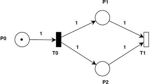
The dynamics of the Petri net model are described by the changes in markings and system states influenced by the transition firings. Transitions can fire and cause changes in system states only when they are enabled. A transition t is said to be enabled only when each of its input places contains W(p,t) token(s), where W(p,t) is the weight of the arc from place p to transition t. Once a transition is enabled it will fire and remove W(p,t) tokens from all its input places and insert W(t,p) tokens into each of its output places, where w(t,p) is the weight of the arc from transition t to place p.

Thus, starting from the initial marking M₀ the firing of transitions leads to a sequence of markings that can be reached from the initial marking. This dynamic behavior of a Timed Petri net can be used to study the system behavior and analyze the different qualitative parameters, that is, safety, liveness, or deadlock-free by using the following Petri net-based concepts before actual system development.

3.1.1. Reachability

Is useful for checking whether the Petri net model reaches a particular marking or state and studying the dynamic behavior of the modelled system using the Petri net model. When an enabled transition fires it causes changes in the marking of the Petri net as a result of the change in the token count in the input and output places of the fired transition. A marking M' is said to be reachable from marking M if there exists a sequence of transition firings ${\sigma }_M\mathrm{ }$ that changes the marking of the Petri net from M to M'. Thus, proving the reachability of the marking M' from M. Mathematically, reachability can be represented as follows: $$M\left[{\sigma }_M\right.〉M\prime$$

3.1.2. Liveness

Is used to detect the absence of deadlock in the system. Liveness is used to verify that in any Petri net marking M there exists at least one transition t that is enabled and fires to lead the Petri net to a new marking M'. Thus, guarantees a deadlock free situation. The liveness property is associated with the transition of the Petri net model. Mathematically, liveness can be represented as follows: $$\forall \mathrm{M},\text{∃t ϵ T},\text{such that M}\stackrel{t}{\to }\mathrm{M}\prime$$

3.1.3. Boundedness

Defines a Petri net as bounded if and only if the number of tokens in each place does not exceed a certain number, say K, for any marking M reachable from the initial marking M₀ using reachability graph. It is associated with the places of the Petri net model. Mathematically, boundedness can be represented as follows: $$M\left(p\right)\le K$$

Here, $M(p$) represents the token count of place p in the marking M and the formula states that the token count should not exceed the bound K. The Boundedness property is useful for checking the finiteness of the Petri net model and thus, is used to verify the safety property of a system.

3.1.4. SPIN

SPIN (Ben-Ari, 2010) model checker which stands for ‘Simple Promela Interpreter’ is an automated verification tool for verifying the logical correctness of concurrent, distributed and asynchronous software systems. SPIN was developed at Bell Labs in 1980 and it is an open-source software, freely available and continues to evolve. The systems to be verified are represented as Process Meta Language (PROMELA) models interpreted by SPIN as a finite state model.

PROMELA (Basic Spin Manual, 2017; Concise PROMELA Reference, 1997) is a modelling language for defining distributed systems as finite-state system models to be interpreted to satisfy critical system properties. The PROMELA program represents a process that consists of name, local variables, formal variables and sequence of statements and supports important concepts or operations such as parallel, repetition, concurrency and sending and receiving messages. The execution of the PROMELA model using SPIN generates a set of all reachable states of the modelled system, which are further analyzed and subjected to exhaustive verification of system specifications.

3.2. Temporal logic

Temporal logic is a system of rules and symbolism used to specify and reason the properties of a system over time. System properties are considered propositions in temporal logic and are represented as a temporal formula for verification. A proposition is a declarative sentence usually denoted by the letters p, q and r that is either true or false. Linear temporal logic (Ding et al., 2014) and computational tree logic (CTL) (van Leeuwen, 1991) are the two types of commonly used temporal logic. Different model checkers support either these temporal logics or extensions of these common temporal logics. SPIN supports LTL in expressing the system specifications for verification.

Linear temporal logic includes connectives that allow modelling or referring to the system’s future states. It represents time as a sequence of states and, extends to the future. As the future is not known, LTL considers several paths, representing different possibilities of the future, and any one of these paths may be the actual path (Huth & Ryan, 2004). Common LTL connectives are as follows: X means ’next state’, F means ’some Future state’ eventually(< >)’, G means ’all future states’ globally([]), U means ‘Until’, R means ’Release’ and W means ’Weak-until’. LTL also supports binary logical operators such as: not(!), or(ǁ) and(&&), imply(→) and equivalence (↔). In this study, LTL was used to specify the system properties and was subjected to verification. Hence, let us consider a few examples to understand the interpretation of the LTL formula.

1. Formula [](p) (read as ‘globally p’)states that at any point in an execution, it is sure that proposition ‘p’ is always true.

2. Formula < >(p) (read as ‘eventually p’) states that at any point in an execution, it is guaranteed that proposition ‘P’ will eventually be true.

3. Formula Xp states that proposition p is true in the next state.

4. Formula p U q (read ‘p until q’), states that proposition p holds until a state is reached where proposition q holds.

Similarly, other operators are used with the propositions and evaluated.

4. Methodology

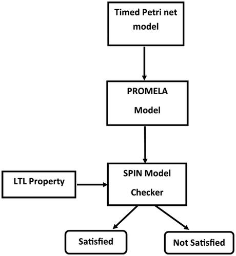
In this section, we discuss the proposed methodology for the transformation of the Timed Petri net into the PROMELA model and conduct a qualitative analysis using the SPIN model checker. Figure 2 shows the proposed methodology for qualitative analysis using a Timed Petri net and SPIN. The proposed approach begins with the Timed Petri net model as the input model and a set of transformation rules is used to automatically transform the Timed Petri net model into the PROMELA model. The proposed approach begins with the Timed Petri net model as the input model and a set of proposed transformation rules are used to automatically transform the input model into the PROMELA model. The system properties to be verified are specified using an LTL representation. Next, the derived PROMELA model and system properties are analyzed using the SPIN model checker which evaluates the properties and indicates whether the property is satisfied or not. Thus, the proposed methodology enables the use of model checking techniques and model checkers in association with Petri net development tools and the environment for system verification.

Figure 2. Methodology for qualitative analysis using Timed Petri net and SPIN.

4.1. Transformation semantics

The process of transforming the Timed Petri net into the PROMELA model is transition centered, based upon the enabling and firing of each transition. The transformation focuses on the main Petri net elements places, transitions, tokens and input and output arcs. The mapping of these Timed Petri net elements is discussed as follows:

• Mapping of Places and tokens: Each place in the Timed Petri net was mapped into a PROMELA variable. The name of this variable is the same as that of the place name. The token count in each place was mapped as the initial value of the corresponding PROMELA variable representing the place.

• Mapping of Transition: The transformation semantics of a transition is the core part of this transformation process. Each transition in the Timed Petri net is mapped into a PROMELA variable, timed transitions are initialized to their transition rates and immediate transitions are initialized to zero. This transition rate represents the concept of time during the execution of the PROMELA model. For each transition, the enabling and firing cases were identified and mapped into PROMELA instructions. Thus, the transition mapping process must consider two main aspects. First, it must identify when a transition is enabled and second the implementation of the firing condition. A transition is enabled if all of its input places have a token, and when an enabled transition fires token is added to all of its output places. Thus, we can consider the different enabling and firing conditions based on the number of input and output places of each transition. The different transition enabling and firing cases to be considered for the transformation are discussed in Subsection 4.2.

• Mapping of Arc: The Petri net arc connects places and transitions, which are used to identify the set of input and output places of each transition. These sets of input and output places are essential for implementing different enabling and firing cases for each transition.

4.2. Transition enabling/firing cases

In the Petri net model, different cases exist when a transition is enabled and fired. As the proposed approach is transition centered, we considered all the different cases in the transformation process. Figure 3 depicts the different cases that exist for the transition to enable and fire. In the Timed Petri net model, the timing information of each transition must also be considered in these cases. To handle timing-related behavior we consider the local time in each transition that represents the transition rate or the time when the transition can fire and a global timer representing the system time. Thus, in the transformation algorithm, it is assumed that when the global time exceeds the local time of a transition, it can fire.

Figure 3. Transition enabling and firing cases.

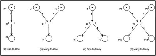
Case (a) is one-to-one, and transition T0 has one input and one output place. The transition is enabled if there is a token in the input place and the global timer is greater than the local transition time. On firing, a token is deleted from the input place and inserted into the output place. This case represents the sequential flow within the system.

Case (b) is many-to-one, and transition T1 has two inputs and one output place. The transition is enabled only when both input places have a token and the global timer is greater than the local transition time. After firing, a token is deleted from all the input places and a token is inserted in the output place. This case represents a system scenario in which more than one condition must be satisfied before an event is executed. The input places represent the conditions and the transition represents event execution.

Case (c) is one-to-many, and transition T2 has one input and two output places. The transition fires when the input place has a token and the global timer is greater than the local transition time. After firing, a token is deleted from the input place and inserted into all output places. The parallel activities of a system can be initiated when this case is executed.

Case (d) is many-to-many, and transition T3 has two input and two output places, and for the transition to enable there must exist a token in both input places and the global timer is greater than the local transition time. After firing, a token is deleted from the input places and tokens are inserted in all the output places. This case a depicts the combination of cases (b) and (c).

For the proper implementation of the transformation process, we must ensure that the firing of a transition is an atomic activity. Hence, once the firing of a transition begins deleting the tokens from the input places and inserting the token into the output place must be completed contiguously. The PROMELA rules for checking the four cases are as follows:

• Case(a): if enable(P0)→fire(++P1) && fire(–P0) [Preset = Postset = 1]

• Case(b): if enable(P2)&&enable(P3)→fire(++P4)&& fire(- -P2)&& fire(- - P3) [Preset >1, Postset = 1]

• Case(c): if enable(P5)→fire(++P6)&& fire(++P7)&& fire(- -P5)

  [Preset = 1,Postset > 1].

• Case(d): if enable(P8)&&enable(P9)→fire(++P10)&& fire(++P11)&&

  fire(- -P8) && fire(- -P9).

  [Preset > 1, Postset > 1].

In each case, enable() represents the process of checking whether a transition is enabled or not. In this process, enable() considers the input place of the transition as a parameter and checks the token count in the input place. This process is repeated for all the input places of a transition. If the token count is greater than zero in all input places and the global timer is greater than the local transition time, then, the transition is considered enabled and ready to fire.

Similarly, fire() represents the process of firing enabled transition. In this process, fire() inserts tokens in all output places by incrementing their token count by one and deleting tokens from all input places by decrementing their token count by one of the enabled transitions. These input and output places are represented as the parameters in fire() with ‘++’ indicating token insertion and ‘- -’ indicating token deletion in the respective places.

4.3. Implementation details

The transformation of the Timed Petri net into the SPIN PROMELA model is implemented using the Java language and DOM (Document Object Model) parser. DOM (JavaTPoint, 2023) is a programming interface for HTML (HyperText Markup Language) and Extensible markup language (XML) documents. It defines the logical structure of documents and how a document is accessed and manipulated. The DOM Parser provides the ability to parse the XML source code from a string to a DOM document. The XMI representation of the Timed Petri net is the input model subjected to parsing using the DOM parser. The DOM parser identifies Timed Petri net elements that are represented as XMI nodes in the input XMI file and extract each of the places, transitions and arc elements to be stored as a nodelist. Different data related to these elements such as node ID, names and token count of places, are also extracted to be represented as attributes in the final output model.

The proposed transformation semantics are implemented separately for each of the Petri net elements using JAVA instructions. For every extracted Petri net place a PROMELA variable is created with the token count as the variable initial value. Similarly, Java-based instructions are written for each transition to implement the mapping of transition enabling and firing into the PROMELA instructions. In this direction, two sets are created to represent the input places called (Preset) and the output places called (Postset) for each transition extracted from the input file.

To create these transitions Preset and Postset the Petri net arc nodelist was used, and the source and target attributes were extracted from each arc. If the target of an arc is a transition element, then the source of that arc, which is a place element, is considered as the preset element of that transition and added to the Preset. Similarly, if the source of an arc is a transition element then the target of that arc which is a place element, is considered as the postset element of that transition and added into the Postset. This process was continued for each transition for every arc. The created Preset and Postset elements are used to implement the transition enabling and firing rules for each transition as discussed in Subsection 4.2.

Once the Petri net elements and data are parsed the corresponding PROMELA elements and instructions are written into a text file. The SPIN model checker accepts the PROMELA model as a text file, thus, the transformation of Petri net elements is written into a text file. Here, the Java-supported file writer class is used to write the text-oriented data for the extracted Petri net elements and their attributes as PROMELA instructions to the output file. The file writer is a class of Java input output packages used to write character-oriented data to a file. The output text file was analyzed using the SPIN model checker to verify different system properties.

The algorithm for the proposed transformation of Timed Petri net elements into PROMELA elements is shown in Algorithm 1.

Algorithm 1.

Transformation of Timed Petri net elements into PROMELA elements

Require: Timed Petri net XMI file with set of Places P, Set of transitions T, Set ofarcs A

Ensure: PROMELA Text file

1: Initialize timer = 1 representing global time

2: for each Petri net place Pi in P do

3: create a variable, set the name of the variable as place Pi.name

4: if (there exists a token in Place Pi) then

5: initialize the variable to token count

6: else

7: initialize the variable to 0

8: end if

9: end for

10: for each Petri net transition Ti in T do

11: create a variable, set the name of the variable as transition Ti.name

12: initialize the variable to transition rate, Ti.rate

13: end for

14: for each Petri net transition Ti in T do

15:create an input set of places "Preset"

16:create an output set of places "Postset"

17:for each arc Ai in A do

18:if Ai.sourcenode = Ti.name then

19:Add Ai.targetnode into Postset

20:end if

21:if Ai.targetnode = Ti.name then

22:Add Ai.sourcenode into Preset

23:end if

24:end for

25: if Preset = 1 AND Postset = 1 then

26:if timer > Ti.rate then

27:Implement Case (a)

28:end if

29: end if

30: if Preset > 1 AND Postset = 1 then

31:if timer > Ti.rate then

32:Implement Case (b)

33:end if

34: end if

35: if Preset = 1 AND Postset > 1 then

36:if timer > Ti.rate then

37:Implement Case (c)

38:end if

39: end if

40: if Preset > 1 AND Postset > 1 then

41:if timer > Ti.rate then

42:Implement Case (d)

43:end if

44: end if

45: timer = timer + 1

46: end for

5. Case study

Two case studies were used to run the proposed approach and depict its application in evaluating qualitative properties. The central server computer system was a typical desktop computer with a single processor. The main components of this system are the CPU, connected memory and external I/O devices. The Kanban system is a production system based on the Just-In-Time control method. More details of the case studies are provided in the following sub-sections. The Timed Petri net model of each case study was developed using the PIPE Petri net modelling environment and is transformed into the SPIN model checker PROMELA format for detailed qualitative analysis.

The PROMELA model can be analyzed either by simulation of the system’s execution or by executing LTL specification for verifying system properties using model checking. In the simulation-based analysis the number of simulation steps is indicated and at the end of the simulation, details about the final state that is reached after the simulation is completed are generated. In the LTL approach, the LTL formula for each system property is provided and executed to check whether it is satisfied or not. As a result of LTL execution, SPIN provides a detailed representation of the result in terms of search depth, time required, memory consumption, etc. If the property is not satisfied, the SPIN provides a counterexample that can be used to understand the reason for failure.

In this article, the application of both the simulation and LTL formula is shown separately to verify the safety/boundedness, liveness and system behavioral properties for both case studies in the following sections. To verify the boundedness property of a Timed-Petri net model the execution of PROMELA must ensure that there is no explosion of the token count in the Petri net places. Thus, the token count in each place during the execution must not exceed a finite number ‘K’ which indicates the initial token count of the model to avoid token explosion and indicate that the Petri net is bounded and safe. Furthermore, the PROMELA model is used to predict the liveness property of the Timed Petri net model by ensuring that there is no deadlock in the model during its execution.

5.1. Central server system

The first case study considered is a simple central server system with its main components being the CPU, memory and connected external I/O devices. The jobs for completion circulate within the system and it is assumed that there are a fixed number of jobs for completion. Each job performs a few CPU and I/O activities. The Timed Petri net model of a central server is depicted in Figure 4 and was adopted from the literature (Fortier & Michel, 2002).

Figure 4. Timed Petri net model of the central server system.

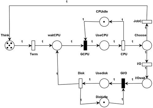
In the Petri net model of the central server, the jobs submitted to the system are represented by tokens in the place Think. Once the job request for service is moved to place waitCPU by the transition Term it has to wait for the CPU to become available. Once the CPU is available the waiting job acquires a CPU that is modelled by moving the token (job) into place UseCPU. The CPU execution cycle is represented by a transition CPU that fires when the job completes its execution and the CPU is idle and available for the next job. Once the job completes it must decide whether it requires further CPU processing or any I/O task, this is represented by the place Choose. If the job requires a CPU it will again be sent to place Think or else it must wait for I/O devices in place I/OWait.

Next, based on the availability of the disk, it will be issued to the job modelled by the presence of a token in place Usedisk and later release of the disk by firing the transition Disk and moving a token in place Diskidle. This sequence shows the I/O(disk) usage of the job in the system. After the completion of the I/O operation, the job will wait for the CPU again in place waitCPU. This process continues for all jobs waiting in the system.

The proposed transformation, being the transition centered, different transitions of the Timed Petri net model, must be mapped to the appropriate PROMELA rules and implement the PROMELA statements.

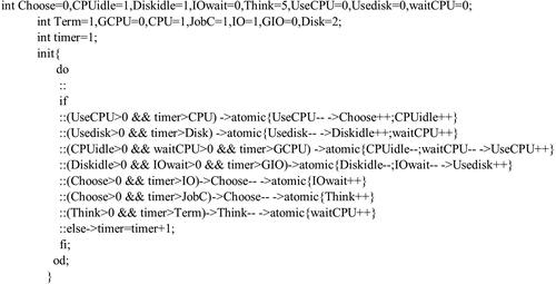
The corresponding PROMELA representation of the central server Petri net model derived using the proposed transformation approach is shown in Figure 5. The places are declared as variables initialized with the token count. The transitions and arcs are represented by PROMELA conditions and statements for execution within do loop and if statements according to the mapped PROMELA cases.

Figure 5. PROMELA model of the central server system.

5.1.1. Experimental results

This subsection discusses the results of the analysis of the transformed Timed Petri net model of the central server system into the PROMELA model using the SPIN tool. The derived PROMELA model was analyzed to verify the boundedness, liveness/deadlock and a few behavioral system properties of the system. Because SPIN supports the verification of boundedness and liveness/deadlock properties using both the simulation method and LTL specifications, this study demonstrates the result of both techniques to verify these properties. However, the behavioral properties of the system were verified using only the LTL specifications. Thus, this section presents the result of the verification of different system properties using simulations and LTL specifications.

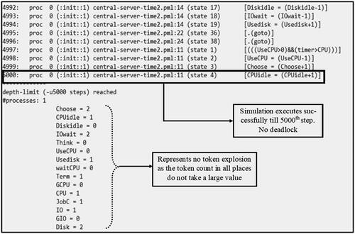
5.1.1.1. Verifying system properties using simulation

To verify the boundedness and liveness/deadlock property of the central server system a simulation method with 5000 steps was performed on the PROMELA model using SPIN and it was observed that at step 5000, there was no token explosion in any of the places. In addition, because the simulation executes for all 5000 steps it also satisfies the liveness property and indicates that the system is deadlock-free. Experiments for other higher step values that is for more than 5000 steps were also conducted and it was observed that the boundedness and liveness properties were still satisfied. The results for 5000 steps are shown in Figure 6, however for other higher step values similar results are obtained thus proving the boundedness and liveness property of the system.

Figure 6. SPIN result of central server verifying boundedness and deadlock using Simulation.

5.1.1.2. Verifying system properties using LTL specifications

Different system properties checked using LTL include: (1) boundedness: The LTL formula represents the condition in which the token count in each of the places is never greater than the initial token count of the model. Here, the initial token count is 7 thus the LTL specification checks that the token count in each place does not always exceed 7. (2) Deadlock: the LTL formula for checking the deadlock situation indicates that always in the system there is someplace whose token count is greater than 0 thus enabling its following transition to fire. This keeps the system alive as either of the transitions is enabled. (3) Mutual exclusive: Check that the system resource CPU and disk are used by only one process at a time. Mutual exclusivity is used to check whether the CPU is used by only one task at a given time. The mutual exclusive property for transitions GCPU and CPU is verified by verifying that the preconditions for enabling the transitions are not satisfied simultaneously. (4) The system buffer is not overloaded with the jobs: Assuming that the initial number of jobs is 5, we check that the number of jobs waiting in the buffer does not exceed 5. (5) Parallel process operations using a CPU and disk simultaneously are possible.

Table 1 lists the different system properties of the central server, its corresponding LTL specification and the result of the execution of the LTL specification. Here, each LTL specification is identified by the name ‘p1’, any valid name can be given to each specification.

Table 1. Different system properties of the central server were verified using LTL.

Property	LTL specification	Result
1	ltl p1{ [](!((Choose > 7) ǁ (CPUidle > 7) ǁ (Diskidle > 7) ǁ (IOwait > 7) ǁ (Think > 7)ǁ (UseCPU > 7) ǁ (Usedisk > 7) ǁ (waitCPU > 7)))}	Zero error
2	ltl p1{ [](< >((Choose > 0) ǁ (CPUidle > 0) ǁ (Diskidle > 0) ǁ (IOwait > 0) ǁ (Think > 0) ǁ (UseCPU > 0) ǁ (Usedisk > 0) ǁ (waitCPU > 0)))}	Zero error
3	ltl p1{ [] (!((CPUidle > 0)&& (UseCPU > 0)))}	Zero error
4	ltl p1{ [] (!(waitCPU > 5))}	Zero error
5	ltl p1{ [] (!((UseCPU > 0) && (Usedisk > 0)))}	Assertion violation

From Table 1 and the LTL analysis results, it is observed that properties (1) to (4) give zero error, which means that the property is satisfied by the model in the process of evaluation by the model checker, thus indicating the satisfaction of properties (1) to (4). Execution of Property (5) assertion violation occurs, which means that the LTL specifications of this property are violated at some stage of execution. This indicates that the token count in places UseCPU and Usedisk is greater than zero simultaneously in some instances of execution, which is the negation of the specified property. This proves that parallel operation of processes using the CPU and disk simultaneously is possible.

5.2. Kanban system

In the second case study, a production system from the manufacturing domain was selected to verify the system properties using the SPIN model checker. A Kanban system is based on the pull strategy in the production system, which is based on the requirements and any new product or part of the product is generated only when there is a demand for it. The Kanban system adopted in this study was inspired by references (Viswanadham & Narahari, 1992) and (Marsan et al., 1995). A linear collection of production cells is used in the Kanban system with every cell accountable for generating and handling unique parts. Each cell has an input and output buffer and a bulletin board with a fixed number of cards (k) to represent the number of parts within a cell. Part arrives in the cell only if there is a card in the bulletin board. Each cell follows a just-in-time strategy and thus, produces a part only when there is a requirement for it from the next cell. The cells were linearly connected to create an n-cell Kanban system.

The Petri net model of a 2-cell Kanban system is shown in Figure 7, and the descriptions of the places and transitions are given in Table 2. Within each cell Ci, whenever a part arrives in the input buffer indicated by a token in the place Inbuff_i, the availability of the machine is checked with the presence of a token in the place Machine_iidle. If the machine is free, the part is processed and sets the machine as busy by inserting a token in the place Machine_i and after the processing task, the part is inserted into the output buffer of the cell indicated by the token in the place Outbuff_i.

Figure 7. Timed Petri net model of 2-cell Kanban system.

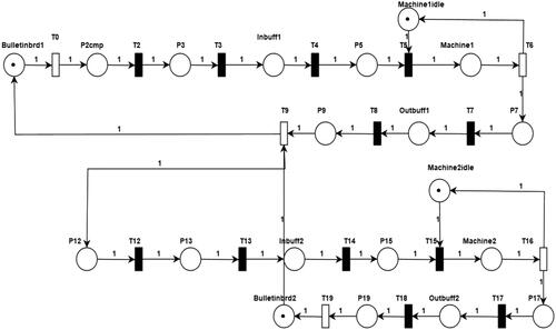
Table 2. Kanban Petri net model places and transitions description.

Element	Description
Bulletinbrd1 & Bulletinbrd2	Represent the bulletin board with tokens within it represents the number of the cards in the cell1 & cell2
Machine1idle & Machine2idle	Represents the condition of the cell, a token here represents the cell Ci is idle
Machine1 & Machine2	Represents the condition of the cell, a token here represents the cell Ci is busy
Inbuff1 & Inbuff2	Represent the input buffer of a cell1 & cell2
Outbuff1 & Outbuff2	Represent the output buffer of a cell1 & cell2

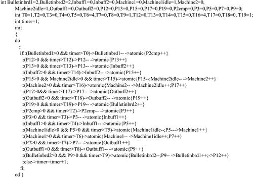
The corresponding PROMELA representation of the 2-cell Kanban system Petri net model derived from the proposed transformation approach is shown in Figure 8.

Figure 8. PROMELA model of the 2-cell Kanban system.

5.2.1. Experimental results

This subsection discusses the results from the analysis of the transformed Timed Petri net model of the 2-cell Kanban system into the PROMELA model to verify the boundedness and liveness properties, as well as a few behavioral properties of the system. The boundedness and liveness/deadlock properties were verified using both simulation and LTL specifications. The behavioral properties were verified using only LTL specifications. This section presents the result of the verification of different system properties using simulations and LTL specifications.

5.2.1.1. Verify system properties using simulation

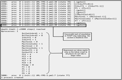
The boundedness property verification was performed using a simulation of 2-cell Kanban Petri net models. A simulation with 5000 steps was performed, and it was observed that there was no token explosion in any of the places of the model. Similarly, because the simulation executes for all 5000 steps it also satisfies the liveness property, and thus, the system is deadlock-free. Experiments for higher step values, that is for more than 5000 steps were also conducted, and it was observed that the boundedness and liveness properties were still satisfied. The results of the simulation for 5000 steps are shown in Figure 9, however for other higher step values similar results are obtained, thus, proving the satisfaction of the boundedness and liveness properties in the Petri net model.

Figure 9. SPIN result of 2-cell Kanban system verifying boundedness and deadlock property using simulation.

5.2.1.2. Verifying system properties using LTL specifications

Different system properties checked using LTL include: (1) boundedness: The LTL formula represents the condition in which the token count in each of the places is never greater than the initial token count of the model. Here, for the 2-cell Kanban system, the initial token count is six, thus the LTL specification checks that the token count in each place does not always exceed six. (2) Deadlock: The LTL formula for checking the deadlock situation indicates that always in the system there is someplace whose token count is greater than 0, thus enabling its following transition to fire. This keeps the system alive as either of the transitions is enabled. (3) The number of jobs in the system was always equal to the card count. (4) A part is transferred into the input buffer of cell C_i only when there is a part in the output buffer of cell C{_i-1} and the bulletin board of cell C_i has a card.

Table 3 lists the different system properties of the 2-cell Kanban system, its corresponding LTL specification, and the result of the execution of the LTL specification.

Table 3. Different system properties of the 2-cell Kanban system verified using LTL.

Property	LTL specification	Result
1	ltl p1{ [](!((Bulletinbrd1 > 6) ǁ (Bulletinbrd2 > 6) ǁ (Inbuff1 > 6)k(Inbuff2 > 6) ǁ (Machine1 > 6) ǁ (Machine1idle > 6) ǁ (Machine2 > 6) ǁ (Machine2idle > 6) ǁ (Outbuff1 > 6) ǁ (Outbuff2 > 6)k(P12 > 6) ǁ (P13 > 6) ǁ (P15 > 6) ǁ (P17 > 6) ǁ (P19 > 6) ǁ (P2cmp > 6) ǁ (P3 > 6) ǁ (P5 > 6) ǁ (P7 > 6) ǁ (P9 > 6)))}	Zero error
2	ltl p1{ [](< >((Bulletinbrd1 > 0) ǁ (Bulletinbrd2 > 0) ǁ (Inbuff1 > 0)k(Inbuff2 > 0)k(Machine1 > 0) ǁ (Machine1idle > 0) ǁ (Machine2 > 0) ǁ (Machine2idle > 0)k(Outbuff1 > 0) ǁ(Outbuff2 > 0) ǁ (P12 > 0) ǁ (P13 > 0) ǁ (P15 > 0) ǁ (P17 > 0) ǁ (P19 > 0)ǁ (P2cmp > 0) ǁ (P3 > 0)k(P5 > 0) ǁ (P7 > 0) ǁ (P9 > 0)))}	Zero error
3	ltl p1{[](!(Inbuff1 > 2))}	Zero error
4	ltl p1{!(< >((Outbuff1 > 0)&& (Bulletinbrd2 > 0))→(< >(Inbuff2 > 0)))}	Assertion violation

From Table 3. The LTL analysis results show that, properties (1) to (3) give zero error, which means that the property is satisfied by the model in the process of evaluation by the model checker, thus, indicating the satisfaction of properties (1) to (3). Execution of Property (4) assertion violation occurs, which means that the LTL specifications of this property are violated at some stage of execution. This indicates that, eventually during the execution a token is inserted in places Outbuff1 and Bulletinbrd2, thus, enabling the firing of the transition T9 and inserting the token in the place Inbuff2 in some instances of execution which is the negation of the property specified. This proves the satisfaction of property (4).

Thus, from the results, it can be observed that the proposed approach is effective in using the Timed Petri net model and SPIN model checking technique to verify different system properties.

6. Conclusion

In this study, an automated approach for the qualitative analysis of a real-time system using the Timed Petri net model and SPIN model checker is proposed. This article illustrates the system representation using the Timed Petri net model and its transformation into the SPIN PROMELA model to verify system properties. The proposed approach contributes to the qualitative analysis of system properties such as deadlock, boundedness, safety and other system dynamic behavioral properties at the initial-stage of system development. In this study, SPIN supported both methods, and the execution of the LTL specification and simulation were used to perform a qualitative analysis of the system properties using the derived PROMELA model. The proposed approach has the advantage of verifying real-world systems from diverse domains such as networks, communication, manufacturing and embedded systems, using existing Petri net tools and mainstream model checkers.

To demonstrate the effectiveness of the proposed approach, the Timed Petri net models of two case studies were considered for evaluating boundedness, liveness properties and system behavioral properties using simulation and LTL specifications techniques. This approach proposes that in the design stage of system development, formal system designs can be used to represent the system and study its behavior. Thus, the main motivation of this approach is to enable system verification using formal modelling techniques to enhance the system design and quality. In addition, the proposed approach is used to bridge the gap between the existing commonly used formal modelling domains, the Timed Petri net and SPIN to verify the real-time system properties.

Authors’ contributions

Tanuja Shailesh: Conceptualization, design, analysis and drafting; Tanuja Shailesh and Ashalatha Nayak: writing review and editing; Tanuja Shailesh, Ashalatha Nayak and Devi Prasad: critical revision and final approval of the version to be published.

Disclosure statement

The authors declare no potential conflict of interest.

Data availability statement

The authors agree to share the data upon reasonable request.

Additional information

Funding

No funding was received.

Notes on contributors

Tanuja Shailesh

Tanuja Shailesh, received B.E degree in Computer Science and Engineering from VTU University in 2002 and M.Tech. and Ph.D. in Computer Science from MIT, MAHE Manipal. She is also a Assistant professor in the Computer Science and Engineering Department at the MIT Manipal. Her research interests include UML Models, Software performance engineering and formal model-based designs and analysis.

Ashalatha Nayak

Ashalatha Nayak, is a Professor, CSE Department, Manipal Institute of Technology Manipal. Did her B Tech, M Tech and Ph. D. in Computer Science from NMAM Institute of Technology Nitte, Manipal Institute of Technology Manipal and IIT Kharagpur respectively. She has authored/co-authored more than 35 technical articles in refereed journals and conferences. Her research interests include UML Models and Object Oriented System Development, Model-Based Analysis and Model-Based Testing, Information security and Enterprise architecture.

Devi Prasad

Devi Prasad, is an independent Consultant in Software design and development services. He has a Ph.D. degree from MNNIT Allahabad and his research thesis involved the development of denotational-style semantics for a statically typed aspect-oriented programming language supplemented with a meta-model based on the UML 2 standard for specifying aspects in requirements specification and software design. His general research interests include the application of semi-formal methods in software development. He is specifically interested in the application of program- verification technology. He has experience in using Dafny for program development and the SPIN model checker for software verification.

References

- Adalid, D., Salmerón, A., Gallardo, M. d M., & Merino, P. (2014). Using spin for automated debugging of infinite executions of java programs. Journal of Systems and Software, 90, 61–75. https://doi.org/10.1016/j.jss.2013.10.056
- Alam, D. M., & He, X. (2017). A method to analyze predicate transition nets using spin model checker. International Journal of Software Engineering and Knowledge Engineering, 27(09n10), 1455–1481. https://doi.org/10.1142/S021819401740006X
- Argote García, G., Clarke, P. J., He, X., Fu, Y., & Shi, L. (2008). A formal approach for translating a sam architecture to PROMELA. 20th International Conference on Software Engineering and Knowledge Engineering (pp. 440–447). Knowledge Systems Institute (KSI).
- Asankhaya, S. (2013). End to end verification and validation with spin. CoRR.
- Basic Spin Manual. (2017, August 3). Manual. https://spinroot.com/spin/man/html
- Bause, F., & Kritzinger, P. (2013). Stochastic petri nets -An introduction to the theory. Vieweg. ISBN 3-528-15535-3.
- Behrmann, G., David, A., & Larsen, K. G. A. (2004). A tutorial on uppaal (pp. 200–236). Springer Berlin Heidelberg. https://doi.org/10.1007/978-3-540-30080-97
- Ben-Ari, M. M. (2010). A primer on model checking. ACM Inroads, 1(1), 40–47. https://doi.org/10.1145/1721933.1721950
- Besnard, V., Teodorov, C., Jouault, F., Brun, M., & Dhaussy, P. (2021). Unified verification and monitoring of executable UML specifications. a transformation-free approach. Software and Systems Modeling, 20(6), 1825–1855. https://doi.org/10.1007/s10270-021-00923-9
- Byg, J., Jørgensen, K. Y., & Srba, J. (2009). TAPAAL: Editor, simulator and verifier of timed-arc petri nets. In Z. Liu, A. P. Ravn (Ed.), Automated technology for verification and analysis (pp. 84–89). Springer Berlin Heidelberg.
- Chaichompoo, O., Thongtak, A., & Vatanawood, W. (2017). Transformation of time petri net into PROMELA [Paper presentation]. 11th International Conference on Telecommunication Systems Services and Applications (TSSA) (p. 1). IEEE. https://doi.org/10.1109/TSSA.2017.8272928
- Chang, L., & He, X. (2015). A methodology to analyze multi-agent systems modeled in high level petri nets. International Journal of Software Engineering and Knowledge Engineering, 25(07), 1199–1235. https://doi.org/10.1142/S0218194015500230
- Cimatti, A., Clarke, E. M., Giunchiglia, E., Giunchiglia, F., Pistore, M., Roveri, M., Sebastiani, R., & Tacchella, A. (2002). NuSMV 2: An opensource tool for symbolic model checking [Paper presentation]. Proceedings of the 14th International Conference on Computer Aided Verification (pp. 359–364). Springer Berlin Heidelberg.
- Clarke, E., Grumberg, O., & Peled, D. (2001). Model checking. MIT Press.
- Concise PROMELA Reference. (1997). https://www.cse.msu.edu/∼cse470/ promela manual/quick.html.
- Ding, X., Smith, S. L., Belta, C., & Rus, D. (2014). Optimal control of markov decision processes with linear temporal logic constraints. IEEE Transactions on Automatic Control, 59(5), 1244–1257. https://doi.org/10.1109/TAC.2014.2298143
- Dingle, N., William, K., & Tamas, S. (2009). PIPE2 a tool for the performance evaluation of generalised stochastic Petri Nets. ACM SIGMETRICS Performance Evaluation Review, 36(4), 34–39. https://doi.org/10.1145/1530873.1530881
- dos Santos, L. B. R., de Santiago Júnior, V. A., & Vijaykumar, N. L. (2014). Transformation of UML behavioral diagrams to support software model checking [Paper presentation]. Proceedings 11th International Workshop on Formal Engineering Approaches to Software Components and Architectures (pp. 133–142). Open Publishing Association.
- Fernandes, F., & Song, M. (2014). UML-checker: An approach for verifying uml behavioral diagrams. Journal of Software, 9(5), 1229–1236. https://doi.org/10.4304/jsw.9.5.1229-1236
- Fortier, P. J., & Michel, H. (2002). Computer systems performance evaluation and prediction. Butterworth-Heinemann.
- Gardey, G., Lime, D., Magnin, M., & Olivier (H.) R. (2005). Romeo: A tool for analyzing time petri nets. In K. Etessami & S. K. Rajamani (Eds.), Computer Aided Verification (pp.418–423). Springer, Berlin, Heidelberg.
- Gerogiannis, V., Kameas, A., & Pintelas, P. (1998). Comparative study and categorization of high-level petri nets. Journal of Systems and Software, 43(2), 133–160. https://doi.org/10.1016/S0164-1212(98)10028-6
- Grobelna, I., & Szcześniak, P. (2022). Model checking autonomous components within electric power systems specified by interpreted petri nets. Sensors, 22(18), 6936.
- Hamman, S. T., Hopkinson, K. M., & Fadul, J. E. (2016). A model checking approach to testing the reliability of smart grid protection systems. IEEE Transactions on Power Delivery, 32(6), 1–1. https://doi.org/10.1109/TPWRD.2016.2635480
- He, L., Liu, G., & Zhou, M. (2023). Petri-net-based model checking for privacy-critical multiagent systems. IEEE Transactions on Computational Social Systems, 10(2), 563–576. https://doi.org/10.1109/TCSS.2022.3164052
- Holzmann, G. J. (1997). The model checker spin. IEEE Transactions on Software Engineering, 23(5), 279–295. https://doi.org/10.1109/32.588521
- Huth, M., & Ryan, M. (2004). Logic in computer science: Modelling and reasoning about systems. Cambridge University Press.
- JavaTPoint. (2023). Java DOM, JavaTPoint. https://www.javatpoint.com/java-dom.
- Kawises, J., & Vatanawood, W. (2019). Formalizing time petri nets with metric temporal logic using PROMELA [Paper presentation]. 20th IEEE/ACIS International Conference on Software Engineering, Artificial Intelligence, Networking and Parallel/Distributed Computing (SNPD). IEEE. https://doi.org/10.1109/SNPD.2019.8935861
- Kwiatkowska, M., Norman, G., & Parker, D. (2011). Prism 4.0: Verification of probabilistic real- time systems (pp. 585–591). Computer Aided Verification.
- Lima, V., Talhi, C., Mouheb, D., Debbabi, M., Wang, L., Makan Pourzand. (2009). Formal verification and validation of uml 2.0 sequence diagrams using source and destination of messages. Electronic Notes in Theoretical Computer Science, 254:143–160.
- Lin, C., Huang, C., & Wang, B. (2018). A spin-based model checking for the simple concurrent program on a preemptive RTOS. CoRR. abs/1808.04239. http://arxiv.org/abs/1808.04239.
- Liu Guanjun Petri Nets. (2022). Theoretical models and analysis methods for concurrent systems. Springer Nature. https://doi.org/10.1007/978-981-19-6309-4
- Marsan, M. A., Balbo, G., Conte, G., Donatelli, S., Franceschinis, G. (1995). Modelling with generalised stochastic petri nets. Wiley.
- Mordechai, B. (2013). Mathematical logic for computer science (3rd ed.). Springer.
- Murata, T. (1989). Petri nets: Properties, analysis and applications. Proceedings of the IEEE, 77(4), 541–580. https://doi.org/10.1109/5.24143
- Nakahori, K., & Yamaguchi, S. (2017). A support tool to design iot services with NuSMV [Paper presentation]. 2017 IEEE International Conference on Consumer Electronics (ICCE) (pp. 80–83). IEEE. https://doi.org/10.1109/ICCE.2017.7889238
- Oubelli, M. A., Younsi, N., Amirat, A., et al. (2011, December 13–15). From UML 2.0 sequence diagrams to PROMELE to PROMELA code by graph transformation using atom3 [Paper presentation]. Proceedings of the Third International Conference on Computer Science and its Applications (CIIA'11) (Vol. 825). Saida, Algeria.
- Popova-Zeugmann, L. (2013). Louchka Time Petri nets (pp. 31–137). Springer. https://doi.org/10.1007/978-3-642-41115-1_3
- Ribeiro, O. R., & Fernandes, J. M. (2007). Translating synchronous petri nets into promela for verifying behavioral properties [Paper presentation]. 2007 International Symposium on Industrial Embedded Systems (pp. 266–273). IEEE. https://doi.org/10.1109/SIES.2007.4297344
- Szpyrka, M., Biernacka, A., & Biernacki, J. (2014). Methods of translation of petri nets to NuSMV language. CS&P
- van Leeuwen J (Ed.). (1991). Handbook of theoretical computer science (vol. a): Algorithms and complexity. MIT Press.
- Vernadat, F., Berthomieu, B., Vernadat, F., Berthomieu, B. (2006). Time petri nets analysis with tina [Paper presentation]. Third International Conference on the Quantitative Evaluation of Systems - (QEST'06) (pp. 23–124). IEEE. https://doi.org/10.1109/QEST.2006.56.
- Viswanadham, N., & Narahari, Y. (1992). Performance modeling of automated manufacturing. Prentice-Hall, Inc.
- Vizovitin, N., Nepomniaschy, V., & Stenenko, A. (2017). Application of colored petri nets for verification of scenario control structures in ucm notation. Automatic Control and Computer Sciences, 51(7), 489–497. 12. https://doi.org/10.3103/S0146411617070227
- Wang, J. (1998). Time Petri nets (pp. 63–123). Springer US. https://doi.org/10.1007/978-1-4615-5537-7_4
- Wiśniewski, R., Wojnakowski, M., & Li, Z. (2022). Design and verification of petri-net-based cyber-physical systems oriented toward implementation in field-programmable gate arrays-a case study example. Energies, 16(1), 67.
- Zhang, P., Muccini, H., & Li, B. (2010). A classification and comparison of model checking software architecture techniques. Journal of Systems and Software, 83(5), 723–744. https://doi.org/10.1016/j.jss.2009.11.709