Performance enhancement of an axial flow compressor using active flow control technique

Abstract

This research article focuses on improving the efficiency of an axial flow compressor stage, enhancing the stall margin, and optimizing flow parameters. Utilizing the NACA 65 series rotor airfoil with 12 blades, the study employs numerical simulations using the K-epsilon turbulence model. The model is validated with experimental data under specific boundary conditions, including a total pressure at the intake and a static pressure at the exit, initially set at atmospheric pressure. The outlet static pressure is incrementally increased until the rotor reaches stall. At this stall point, the tip injection method, a well-known active flow control technique, is implemented to mitigate flow instabilities. Injectors are placed at the leading edge of the rotor blades, distributed circumferentially. The tip injection parameters include 0.3% of the total mass flow rate, a pitch angle of 30 degrees and yaw angles ranging from −15 to +15 degrees. The analysis shows a stall margin improvement (SMI) of 14.26% with the 0.3% total mass flow rate injection. A decrease in the yaw angle reduces blockage and promotes smoother flow over the rotor blade, with the optimal stall margin enhancement occurring at an adverse yaw angle of −15 degrees. This study demonstrates significant SMI in the axial flow compressor rotor using specific active flow control parameters, particularly highlighting the critical role of adverse yaw angles in the tip injection method in enhancing stall margin, contributing to overall efficiency and stability.

Keywords:

• NACA
• CFD
• ANSYS-CFX
• axial flow compressor
• stall margin improvement
• tip injection

Reviewing Editor:

• Dr Pham D T, University of Birmingham, United Kingdom of Great Britain and Northern Ireland

Subjects:

• Aerospace Engineering
• Thermodynamics
• Mechanical Engineering

1. Introduction

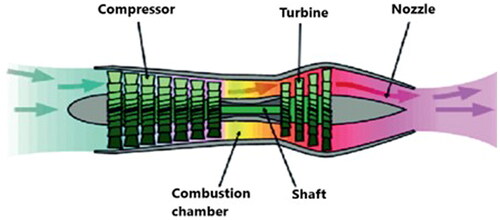
Demand for faster and safer aircraft engines is steadily increasing within the aviation industry. These engines operate on the Brayton cycle, where efficiency is primarily dictated by the performance of compressor and turbine components. An aircraft jet engine in Figure 1 typically comprises several key parts, including the turbine, nozzle, combustion chamber and compressor. Aircraft engines employ two primary compressors: centrifugal (or radial) compressors and axial-flow compressors. Due to their efficiency and performance characteristics, axial-flow compressors are preferred for massive modern turbofan engines. Conversely, centrifugal compressors are typically utilized in applications involving low-pressure, small turbojet engines (Srinivas et al., 2018) when compared to centrifugal compressors, axial compressors offer the advantage of handling a larger mass flow rate at frontal cross-section. This capability, combined with a significant improvement in both compressor pressure ratio and air mass flow rate, results in a notable increase in the engine’s thrust output. These factors represent compelling arguments in favor of the extensive utilization of axial compressors in aircraft jet engines (Vasudeva et al., 2021).

Figure 1. Aircraft engine representation with turbomachinery component.

A compressor’s design point is determined by the rotational speed and pressure ratio where efficiency is optimized. Since engine performance is directly affected by the pressure ratio, compressor developers strive to maximize it. However, as the pressure ratio approaches its maximum, it edges closer to the stall point. Under certain conditions, such as downstream throttling or inlet distortions, stall phenomena may exist in blade passages. This reduces the compressor’s efficiency and shifts its performance within reach of the surge line. Given the significant impact of stall and surge occurrences on compressor performance and overall engine operation, designers must explore methods to minimize or mitigate these phenomena (Taghavi-Zenouz & Ababaf Behbahani, 2018).

As the compressor approaches its stability limits, inevitable phenomena like rotating stalls or surges lead to extreme vibration and a decline in performance. To maximize benefits, optimizing the compressor flow range is crucial (Ahmad et al., 2020). Under certain conditions, it may be acceptable for a few stages of a compressor to operate under rotating stall conditions, albeit at the expense of reduced efficiency (Duc Vo et al. 2008). However, the occurrence of a surge must be entirely prevented, as it is typically irreversible and can result in significant mechanical damage. The mechanism of stall inception is a subject of investigation by many researchers, who explore it through experimental or numerical means (Gourdain et al., 2006; Weichert & Day, 2013). The onset, growth, and propagation of instabilities, such as rotating stall, often occur after several rotations of blade rows within the compressor (Shi et al., 2013). To address these challenges, various methods have been developed to prevent the formation of instabilities. These methods encompass both passive and active approaches, aiming to introduce strategies that broaden the stable operating range of the compressor. By employing such methods, compressor designers seek to enhance performance and reliability while ensuring smoother and more efficient operation across a wider range of operating conditions (Kim et al., 2013; Chen et al., 2013). To improve flow and stabilize the operation of the compressor, active flow control techniques are particularly utilized for axial flow compressor rotor blades. One such technique is the tip injection method, which is implemented on the blade to counteract the formation of vortexes and prevent disruptions to the mainstream flow entering the axial compressor while accepting a slight decline in efficiency (Hiller et al., 2011). The main concept of the active control method was proposed by Epstein et al. (1989). The method involves injecting fluid at the blade tip to rectify blockages or vortex formations, thereby reducing turbulent flow. Key parameters of the tip injector include the injected mass flow rate and momentum, pitch angle, yaw angle, circumferential distribution at leading edge and axial location of the injector in the passage (Wojewodka et al., 2018). By optimizing these parameters, engineers can effectively mitigate instabilities and enhance overall performance of the compressor. Lu et al. (2006) conducted experimental and numerical investigations to explore the effects of air injection on axial compressor performance and its mechanisms concerning stall margin improvement (SMI). Their findings indicate that the physical mechanisms underlying the extension of compressor stall margin through blade row tip injection are twofold. First, injection method retards the upstream movement of the entering flow, thereby influencing the interaction with the tip leakage flow interface. Second, it delays the inception of stall. These mechanisms collectively contribute to enhancing the compressor’s stall margin and improving its overall performance. Khaleghi (2015) organized numerical investigation to explore the influence of air injection on controlling stall, with a specific focus on the NASA Rotor-67. By turning on the end wall injection in an in-stall condition induced by an expanded tip blade, the objective was to gain insights into the underlying physics governing the transition of the compressor from a stall condition and the flow within half of the entire annulus, with particular attention to the rotor blade row operating under stall conditions to a stable state upon activation of air injection. The study investigated how different tip clearance sizes affect compressor stability and performance. Subsequently, high-speed fluid injection was introduced upstream of the blade endwall to assess its effects on compressors with varying tip clearance sizes. Another (Khaleghi et al., 2016) look over the impact of different tip clearance sizes on compressor stability and performance. Subsequently, high-speed fluid injection was introduced upstream of the blade end wall to evaluate its effects on compressors with varying tip clearance sizes. Results indicate that regardless of tip clearance size, tip injection effectively enhances compressor stability and improves the total pressure ratio. However, this enhancement is accompanied by some efficiency loss. Furthermore, the study examined the near-stall end wall flow structures for various tip clearance sizes, both with and without injection. Surprisingly, the tip clearance size was found to have no influence on the compressor stalling mode. Additionally, under certain conditions, injection led to a transition from ‘wall-stall’ to ‘blade-stall,’ highlighting significant impact of injection on compressor behavior and performance.

The specific function of each rotor blade in an axial compressor stage remains complex. Nevertheless, the significance of rotor blades in aircraft engines cannot be overstated. By comprehensively understanding the flow physics and mechanisms governing rotor blades, such as those represented by the NACA 65 series, engineers can effectively optimize compressor performance. This optimization not only enhances engine efficiency but also contributes to improved overall aircraft performance and safety.

It is observed through the literature summary that more research attempts should have been made on both the active and passive flow control techniques on the axial flow compressor. It is also clear that experimentally conducting active and passive control techniques leads to more expensive results. Hence, the numerical simulations of the same control techniques help the researchers predict turbomachinery aerodynamics and efficiency parameters, calculations are also quite easy. The reason for the selection of the active flow control technique is to boost the aerodynamic flow through different rotating machines in a given flow passage. It has also been noted that authors have not attempted to apply the active flow control technique to the rotor blade’s impification and the flow physics surrounding it. Most publications did not discuss the specific flow dynamics and aerodynamics surrounding the rotor blade. Hence, this study aims to rise the flow characteristics of an axial flow compressor by incorporating a tip injector positioned at the leading edges of blades. The injector’s circumferential distribution is carefully considered, and a tip injection equivalent to 0.3% of the total mass flow rate across entire annulus is introduced at the injector inlet. Various turbulence models are employed to ensure optimal grid values for the parameters under investigation.

2. Methodology

2.1. Design of the rotor blade

The rotor blades depicted in Figure 2(a–c) illustrate the hub, mean and tip regions, respectively. Each region’s points were imported into SOLIDWORKS software for further processing. Initially, a plane was created for the hub region with a radius of 135 mm. Subsequently, the rotor blade files for the hub region were imported, and all points were joined to form the blade geometry. This procedure was replicated for the different blade regions by creating planes with tip radius of 180 mm and 224.5 mm, representing the mean and tip regions, respectively. The blade span was measured to be 89.5 mm, as indicated in Table 1. The distance from inlet boundary condition to leading edge of the rotor blade was measured to be 190 mm, while the distance from the trailing edge of rotor blade to the outlet boundary condition was determined to be 430 mm. Finally, all three regions were lofted to generate the 3D representation of the blade, as depicted in Figure 3 below.

Figure 2. (a) Representation of blade’s geometry at hub region (Fukuhara, 1985). (b) Representation of blade’s geometry at mean region (Fukuhara, 1985). (c) Representation of blade’s geometry at tip region (Fukuhara, 1985).

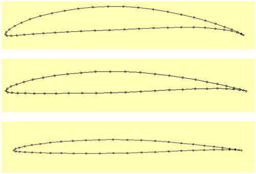
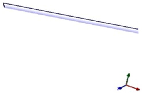
Figure 3. NACA 65 rotor Blade.

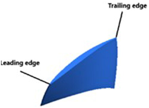
Table 1. Design of axial compressor rotor blade (Fukuhara, 1985).

Description	Design standard
Compressor rotor blades	NACA 65
Distance of Hub rotation from the axis	135 mm
Distance of Tip rotation from the axis	224.5 mm
Wing span	89.5 mm
Rotational speed of the rotor	1300 rpm
Flow Regime	Subsonic
Number of blades	12
Hub-to-tip ratio	0.6
Tip clearance	0.5 mm

The rotor blade model was designed using CATIA V5 R21 software and subsequently imported into the ANSYS-Bladegen module for visualization of the 3D axial flow compressor rotor blade. The numerical analysis of the axial flow compressor revealed that it consists of 12 blades distributed across the entire annulus. The model comprises a hub, where the blades are attached, and a casing to protect the inner components of the axial compressor. In operation, the rotor blade rotates within the aircraft engine, with a hub-to-tip ratio of 0.6 for the blade. Notably, the axial flow compressor operates at low speed, with a rotational speed of 1300 revolutions per minute (RPM). For further reference, the geometry of the model depicted in Figure 3 is mentioned in Table 2.

Table 2. The geometry of the model (Fukuhara, 1985).

Parameter	Hub	Mean	Tip
Radius (mm)	135	180	224.5
Chord length (mm)	106.1	117.8	117.5
Camber (Cl0)	1.30	0.62	0.32
Maximum thickness/chord (%)	10	8	6
Trailing edge thickness/chord (%)	1.41	1.27	1.28
Stagger angle (deg)	31.5	47.2	56.2
Inlet flow angle (deg)	49.1	57	62.5
Exit flow angle (deg)	22.2	44.4	55.8

2.2. Meshing

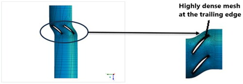
The model is then transferred to the Turbogrid module, and automatically the single-blade passage region is generated. Figure 4 indicates the generated blade passage. The mesh plays a very important role in the simulation for accuracy purposes and Figure 5 represents the distribution of the uniform flow parameter to result in better outcomes. The mesh was performed in the TURBOGRID module, consisting of total nodes of 513,728 and elements of 484,091 for better analysis of rotor blades with a tip clearance of 0.5 mm to obtain a pressure ratio and efficiency of the engine. The offset y⁺ non-dimensionalized distance opts to have fine mesh and to have all the blades in the equidistance, The value of non-dimensionalized distance y⁺ is 10, and the Reynolds number is 5*10 ^+5 for subsonic flow. With the increase in the Reynolds number, there is an increase in efficiency, a minor reduction in the stand, and also an increase in turbulence. The H-grid mesh type is selected to have a structured grid at the interface’s inlet and outflow.

Figure 4. Representation of the mesh formation in turbo grid.

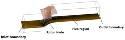
Figure 5. Representation of meshing elements near the rotor blade.

Equation (1)(1) $$y^{+}=\frac{\rho u_{\tau }{y}_{\mathit{\text{wall}}}}{\mu }$$(1) depicts the element count and size selected for the passage in the blade to increase the number of elements and the density of the mesh near the rotor blades. (1) $$y^{+}=\frac{\rho u_{\tau }{y}_{\mathit{\text{wall}}}}{\mu }$$(1)

2.3. Grid independency test

We implemented the grid independence test method to enhance the computational fluid dynamics (CFD) process. In CFD, the goal is to discretize a finite number of grids for numerical analysis, providing approximate solutions to the Navier − Stokes equations based on these grids. To determine the optimal grid resolution, we systematically increased the mesh elements of the blade passage. We calculated the grid point that yielded the most accurate solutions using Equation (2)(2) $$\mathit{\text{Error}} \%=\frac{{\mathrm{\eta }}_{0.6\mathrm{ }\mathit{\text{Million}}\mathrm{ }\mathit{\text{Elements}}}-{\mathrm{\eta }}_{0.5\mathrm{ }\mathit{\text{Million}}\mathrm{ }\mathit{\text{Elements}}}}{{\mathrm{\eta }}_{0.6\mathrm{ }\mathit{\text{Elements}}}}$$(2) . Subsequently, we fixed the mesh elements at 0.5 million to conduct further simulations employing various turbulent models. Figure 6 illustrates the graphical representation of the different mesh element configurations and Table 3 shows the validation of the independence check. (2) $$\mathit{\text{Error}} \%=\frac{{\mathrm{\eta }}_{0.6\mathrm{ }\mathit{\text{Million}}\mathrm{ }\mathit{\text{Elements}}}-{\mathrm{\eta }}_{0.5\mathrm{ }\mathit{\text{Million}}\mathrm{ }\mathit{\text{Elements}}}}{{\mathrm{\eta }}_{0.6\mathrm{ }\mathit{\text{Elements}}}}$$(2)

Figure 6. Representation of the grid independence test with mesh elements vs. pressure ratio.

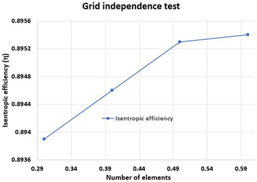
Table 3. Validation of grid independence test.

Mesh elements (millions)	Isentropic efficiency	Error (%)
0.3	0.8939	–
0.4	0.8946	0.0782
0.5	0.8953	0.0781
0.6	0.8954	0.0111

η – Isentropic efficiency

2.4. Boundary conditions

Boundary conditions are crucial in simulations to attain accurate validation of unknowns. At the inlet, the simulation applies a total pressure and temperature set at 288.15 K and flow direction normal to the boundary. Specifically, the total pressure is fixed at 101,325 Pa. This inlet boundary condition remains constant throughout the simulation, regardless of subsequent changes to the outlet boundary condition.

At the exit boundary condition, average static pressure is applied. The average static pressure iteration is initially started with an atmospheric pressure value of 101,325 Pa, and for further iteration, the outlet boundary condition of the average static pressure increases. It increased until the rotor blade attains stall and forms the instability flow in the axial flow compressor rotor blade. Table 3 provides a summary of the numerical simulation results obtained without the injection process.

2.5. Analysis

After the meshing in the Turbogrid module, the data is transferred to the CFX-Pre module for further analysis. The simulation is performed in a steady state with subsonic flow. The fluid opted for is air, an ideal gas and the gauge pressure is assumed to be zero. Heat transferred is adiabatic at all wall surfaces and the inlet flow direction is normal to boundary, with 1300 rpm rotational speed, and 0.5 mm tip clearance. Boundary conditions are imposed, as discussed in Table 4. The simulation begins with different Turbulence models K-epsilon, shear stress transport, RNG K-epsilon, generalized K-Omega and K-Omega. Initially, an atmospheric pressure of 101,325 Pa with the inlet of total pressure and temperature with flow direction normal to boundary and outlet with average static pressure simulations is started, and iteration goes on until mass flow rate and mass and momentum reach constant and they converge at 10^−5. Equations (3)(3) $$\text{Pressure rise coefficient},C_P=\frac{P_{\mathit{\text{Static}}}-P_{\mathit{\text{Total}}}}{0.5\mathrm{*}\rho \mathrm{*}{U}^2}$$(3) and (4)(4) $$\text{Blade speed},U=\frac{\mathit{\text{π*D*N}}}{60}$$(4) are utilized to determine the data required. For a further increase in the average static pressure at the exit boundary condition, there will be a reduction in the mass flow coefficient. The number of maximum iterations is specified as 10,000 iterations, and the RMS residual type has a target of 0.000001. For the rotor blade, it is observed that the stall point is at 101,515 Pa, and tip leakage and vortex breakdown occurred due to instability. Further, the rise in average static pressure represents that the blade gets stalled and the instability in the axial flow compressor. (3) $$\text{Pressure rise coefficient},C_P=\frac{P_{\mathit{\text{Static}}}-P_{\mathit{\text{Total}}}}{0.5\mathrm{*}\rho \mathrm{*}{U}^2}$$(3) (4) $$\text{Blade speed},U=\frac{\mathit{\text{π*D*N}}}{60}$$(4)

Table 4. Boundary condition values without injector.

Inlet boundary conditions of total pressure	Outlet boundary conditions average static pressure	Mass flow coefficient	Pressure rise coefficient	Remarks
101,325	101,325	0.6930	0	Initial point
101,325	101,400	0.6148	0.1954
101,325	101,420	0.5866	0.2476
101,325	101,450	0.5436	0.3257	Design point
101,325	101,480	0.4959	0.4038
101,325	101,505	0.4465	0.4689
101,325	101,515	0.4195	0.4949	Stall point

$\rho$= Density of blade at leading edge

D = Diameter of blade

N = Rotational speed of blade

3. Tip injection method

The key parameters of tip injection flow control are

1. Injected mass flow, velocity and momentum

2. Pitch and yaw angle of the injector

3. Axial location of injectors to the leading edge

4. Circumferential distribution of the injectors

The tip injection method serves as a significant active flow control technique employed to eliminate instabilities within axial flow compressor aircraft engines. This method is deployed in response to blockages that occur in the flow of rotor blade. Blockages arise when the mainstream flow encounters high incidence angles, leading to elevated turbulence levels and impeding the desired efficiency and SMI. Through tip injection, these blockages are addressed, resulting in reduced turbulence and enhanced efficiency, ultimately contributing to improved engine performance and stability.

3.1. Model of tip injector

The tip injector is situated within the shroud region of the blade passage and is designed using CATIA V5 software by creating a plane. Figure 7 illustrates the solid pipe representing the tip injector, characterized by a diameter of 1.5 mm. The injector features two faces for its inlet and outlet, facilitating the imposition of boundary conditions. At the inlet, boundary conditions are specified as mass flow rate and heat transfer at a static temperature, with the flow direction set normal to the boundary condition. Conversely, the outlet boundary conditions are connected to the interface. The wall of the injector is designated as adiabatic, featuring a smooth and no-slip surface. Additionally, the injector remains non-rotating throughout the simulation process.

Figure 7. Representation of the tip injector model.

3.2. Meshing of tip injector

The model of the tip injector was imported into ANSYS-MESH for meshing, aiming to achieve a uniform distribution of a specified parameter and ensure accurate validation. Meshing was performed using the CFX solver preference, employing a multi-zone approach and inflation techniques. The multi-zone meshing strategy was adopted to create a structured mesh in the injector region, covering both end faces. Inflation was applied to refine the body of the injector. The first layer thickness is chosen and the value is 6.224 × 10^−4 and a maximum layer count of 15 layers. Maintaining a mesh element size of 3.3319 mm prioritized high mesh quality to facilitate precise simulations. The resulting mesh consisted of 46,291 nodes and a total of 38,800 elements. This meticulous meshing strategy ensures effective capture of the injector region, enabling accurate analysis and validation of the model’s performance.

3.3. Analysis of tip injector

Following the meshing process in ANSYS-MESH, the tip injector is imported into ANSYS-CFX Pre, as depicted in Figure 8. The injector is maintained in a stationary mode, with boundary conditions at the inlet set to 0.3% of the total mass flow rate of the entire annulus and a static temperature of 288.15 K. The outlet face of the injector is connected to the interface at the shroud region. At the interface, a frozen rotor model is selected with a specified pitch angle of 30 degrees and a yaw angle of 0 degrees. The simulation continues for various average static pressures at the outlet boundary condition of the rotor blade, mirroring conditions without the injection process. Table 5 summarizes the numerical simulation results incorporating the tip injection process.

Figure 8. Representation of tip injector with the blade passage.

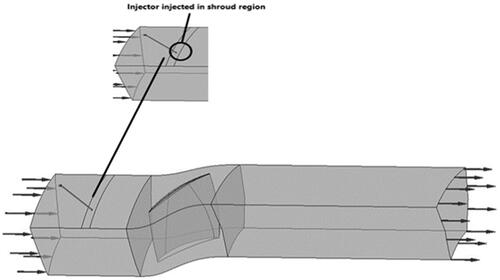
Table 5. Boundary conditions for tip injection method.

Inlet boundary conditions of total pressure	Outlet boundary conditions average static pressure	Mass flow coefficient	Pressure rise coefficient	Remarks
101,325	101,325	0.6930	0	Initial point
101,325	101,400	0.6891	0.1955
101,325	101,450	0.6312	0.2476	Design point
101,325	101,500	0.5602	0.3258
101,325	101,550	0.4613	0.4039
101,325	101,575	0.3622	0.5583	Stall point

4. Results and discussions

The steady simulation of the NACA 65 rotor blade validates the improvement in stall margin. Numerical results are compared with experimental data (Fukuhara, 1985), revealing a notable agreement with the experimental findings, as illustrated in Figure 9. The tip injection method is implemented in the axial compressor to obtain better performance of the engine. SMI is estimated by changing the yaw angle ranging from −15 to +15.

Figure 9. Representation of baseline numerical and experimental validation of mass flow coefficient vs. coefficient of pressure for different turbulent models.

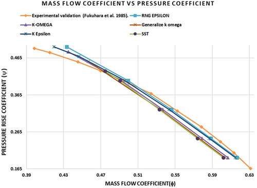
The graph in Figure 9 indicates the performance of the rotor blade, mass flow coefficient vs. pressure rise coefficient for various turbulent flow models: K-epsilon, K-Omega, RNG K-epsilon, generalized k-omega and Shear Stress Transport. It is viewed that increase in average static pressure at the exit boundary condition, there is a decline in mass flow rate and a hike in the pressure rise coefficient (ψ). Similarly, as the mass flow coefficient (ϕ) decreases there is an increase in isentropic efficiency (η) reaching its peak at the design point and then decreases sharply as the system approaches the stall point observed in Figure 10, where mass flow coefficient (ϕ), pressure rise coefficient (ψ) and isentropic efficiency (η) are defined in Equations (5)–(7). The stall point of various turbulent models exhibits variability, contingent upon the turbulence characteristics within the flow. Notably, turbulent models with higher turbulence levels tend to experience early stall occurrences. It is observed that the K-Epsilon turbulent model is closer to the experimental stall point and delay in stall than other turbulence flow models, it is acceptable to use this particular turbulent flow for non-dimensional distances of value 10. Tables 6 and 7 show the percentage error of various turbulence models utilized. For further improvement in the tip injection method, the K-Epsilon turbulence model is finalized for further numerical simulations. (5) $$\text{mass flow coefficient},\left(\varphi \right)=\frac{Q}{\left\{u_t\pi \frac{\left(D^2-D_h^2\right)}{4}\right\}}$$(5) (6) $$\text{Isentropic Efficiency},\left(\eta \right)=\frac{\text{ϕψ}}{\lambda }$$(6) (7) $$\text{shaft power coefficient},\lambda =\frac{L}{\left\{\rho u_t^{3 }\pi \frac{\left(D^2-D_h^2\right)}{8}\right\}}$$(7)

Figure 10. Representation of the baseline results with numerical and experimental validation of mass flow rate coefficient vs. efficiency for different turbulent models.

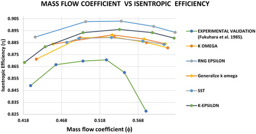
Table 6. Validating errors with experimental data on blade performance.

Turbulent flow	Choking point error (%)	Stall point error (%)
K-epsilon	2.56	4.98
Shear stress transport	4.61	16.03
K-Omega	3.86	8.38
RNG K-Epsilon	2.32	8.05
Generalize k-omega	4.37	12.74

Table 7. Validating errors with experimental data on the efficiency of blades.

Turbulent flow	Initial point (%)	Stall point (%)	Design point (%)
K-Epsilon	6.88	2.24	2.84
Shear stress transport	6.32	4.10	2.11
K-Omega	6.01	2.54	2.15
RNG K-Epsilon	5.14	4.58	3.59
Generalize k-omega	6.38	3.94	2.35

D = Casing diameter

D_h = Hub diameter

L = shaft power

Q = Mass flow rate

U_t = speed of blade tip

ρ = density

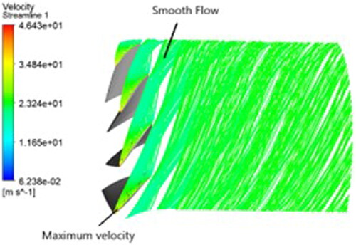
When tip leakage and flow obstruction are absent, a compressor is operating at maximum efficiency, which is represented by the design point. Smooth streamlines inside the blade passage, as observed in Figure 11, highlight the effective flow transfer from one stage to the next and show the fluid flow trajectory across successive stages. Compressors are inherently geared toward achieving high-pressure ratios, and this peak pressure ratio is often approached or attained near the stall point.

Figure 11. Representation of flow at the design point.

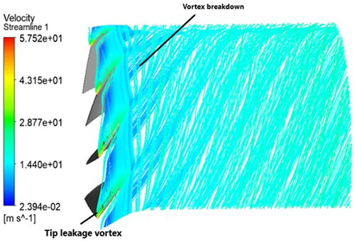
Figure 12 illustrates the flow characteristics at stall point, there is a significant impact on tip leakage flow, leading to blockage of the main flow. The tip leakage vortex (TLV) emerges from the leading edge of the blade and disintegrates within the center region of the flow passage. The compressor hub region experiences the adverse effects of TLV as they move along the blade span. In such scenarios, the flow tends to divert toward the trailing edg and leakage in the front edge. It is observed that although the pressure ratio seems to be at its peak, but the vortex breakdown indicated criteria are negatively impacted, the significant local losses in these region attributes to the increase in diffusion rate which is considered as unpleasant. The efficiency experiences a significant decrease and approaches closer to the surge line. Exploring techniques for preventing the stall and surge phenomena is imperative and crucial.

Figure 12. Representation of the velocity flow at the stall point.

4.1. Improvement in air tip injection

After the implementation of air tip injector in the blade passage at leading edge strategy outlined in Table 8. It was observed noticeable increment in efficiency, pressure ratio and SMI. In this method, there is suppression of pressure loss and vortex breakdown formation, and the graph, Figure 13 elucidates performance of rotor blade with injection at zero yaw angle, it is seen there is a delay in the stall when compared to baseline validation. The physical mechanism to improve the stall margin is to unload the rotor with a decrease in mainstream flow angle. Equation (8)(8) $$\mathrm{\%}{\mathrm{\varphi }}_{\mathit{\text{sm}}}=\frac{({\mathrm{\varphi }}_{\mathit{\text{stall}},\mathit{\text{baseline}}}-{\mathrm{\varphi }}_{\mathit{\text{stall}},\mathit{\text{injection}}})}{{\mathrm{\varphi }}_{\mathit{\text{stall}},\mathit{\text{baseline}}}}\times 100$$(8) gives the SMI value between baseline and injection process. The SMI for zero yaw angle is 10.36%.

Figure 13. Comparison of the baseline validation and tip injection validation at K-epsilon turbulent model.

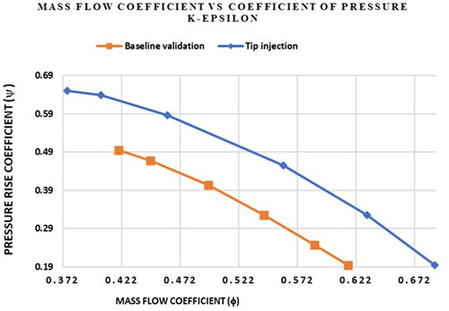
Table 8. Dimension and boundary conditions of tip injector.

Parameter	Dimension
Diameter of injector	1.5 mm
Inlet boundary conditions	0.3% of total mass flow
Outlet boundary conditions	Interface
Pitch angle	30 degrees
Yaw angle	0, +15 and −15 degrees

Stall margin improvement (SMI), (8) $$\mathrm{\%}{\mathrm{\varphi }}_{\mathit{\text{sm}}}=\frac{({\mathrm{\varphi }}_{\mathit{\text{stall}},\mathit{\text{baseline}}}-{\mathrm{\varphi }}_{\mathit{\text{stall}},\mathit{\text{injection}}})}{{\mathrm{\varphi }}_{\mathit{\text{stall}},\mathit{\text{baseline}}}}\times 100$$(8)

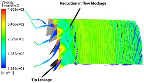
Referring to Figure 14, it becomes evident that injecting into the blade tip region effectively contributes to the spillage and backflow processes that existed earlier, without causing significant blockage to the mainstream. However, some slight blade leading edge spillage may still be seen in passages not exposed to the injectors, which is insufficient to trigger the stall phenomenon. The injector at the blade tip region redirects the trajectory of the TLV toward the mainstream, thereby significantly reducing flow blockage. Therefore, the TLV geometry and design conditions seem very similar. It reduces the aerodynamic losses of blade; flow velocity increases at entry region of blade passage; and the increment has an impact decline in the diffusion factor, which is near to expected values.

Figure 14. Velocity distribution of the tip injector across the rotor blade in the K-epsilon turbulent model.

Figure 15 depicts the performance of the rotor blade at a positive yaw angle of 15 degrees, We obtain the SMI of 8.36%. Similarly, Figure 16 illustrates the negative yaw angle of 15 degrees, and results in an improvement of 14.26%. Upon the comparison of positive and negative yaw angles, it is noticed that the appearance of the physical graph closely resembles the negative yaw angle when compared to the positive yaw angle representing better performance. Table 9 shows the summary of the effect of tip injection and their flow parameter. Similar results have been obtained in Nie et al. (2002) and Taghavi-Zenouz & Ababaf Behbahani (2018).

Table 9. Parametric studies of stall margin.

Yaw angle (degrees)		Stall point mass flow coefficient (ϕstall)	Stall margin improvement (%)
0 Yaw angle	No injection 0.3% injection	0.4195 0.376	10.36
Non zero yaw angle	−15 degrees 15 degrees	0.3596 0.3844	14.26 8.36

The velocity triangles at the near-stall region and design point are shown in Figures 17 and 18. The brown velocity vector indicates the baseline case, the blue velocity vector represents the tip injection, and the black velocity vector depicts the injection flow. At the design point, the injection is parallel to the baseline absolute velocity because there is a drop in the flow velocity. The inlet flow angle (β_injection > β_baseline) is shown in Figure 17. In the throttling process from the design point to the stall point, the proportion of the main flow decreases, and the reduction in the injection flow angle results in a decrease in the inlet flow angle (β_injection < β_baseline) as shown in Figure 18. This leads to the suppression of tip leakage and an improvement in the stall margin and overall efficiency in the compressor rotor.

Figure 15. Mass flow coefficient vs. coefficient of pressure of baseline and injection at a +15 degree yaw angle.

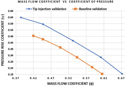
Figure 16. Mass flow coefficient vs. Coefficient of the pressure of baseline and injection in −15 degree yaw angle.

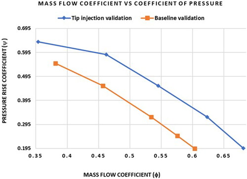
Figure 17. Velocity triangle at tip region design point.

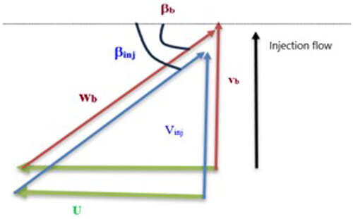
Figure 18. Velocity triangle at tip region near stall region.

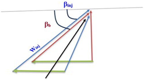
where W_b = Relaive velocity in baseline

 W_inj = Relative velocity in injection

 V_b = Absolute velocity in baseline

 V_inj = Absolute velocity in injection

 U = Blade speed

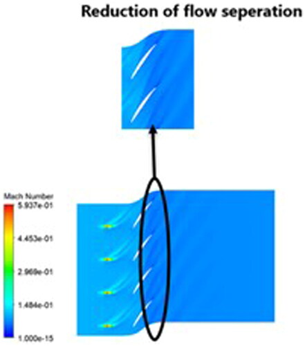
Mach number: The leading edge of the rotor blade produces lift and delivers maximum pressure in an axial flow compressor close to the stall point. This lift impacts the incidence angle and airflow of the incoming flow stream, resulting in the creation of a tip vortex, which causes a sharp drop in flow velocity. The Mach number is about equal to 1. Flow separation occurs at the blade’s trailing edge, as seen in Figure 19. To limit the rotor’s instabilities that arise from the interaction between passing shocks and the boundary layer, the tip injector is placed at the tip of the blade. Notably, the streamline assumes a better aerodynamic shape for a small fraction of the overall mass flow rate with the reduction in tip leakage and flow separation, as illustrated in Figure 20.

Figure 19. Mach number distribution for baseline case.

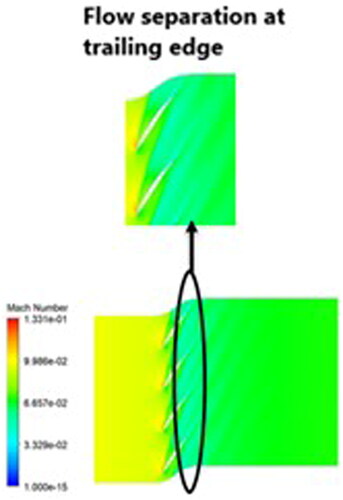
Figure 20. Mach number distribution for tip injection.

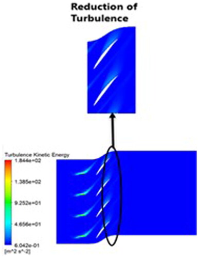
Turbulence: It abruptly surges in turbulence at the mid-span of the blade due to high incidence angle flow and forms a high level of turbulence kinetic energy, this happens when the boundary layer detaches the compressor. It leads to loss of efficiency and performance of the rotor shown in Figure 21. Inherently it involves energy dissipation due to viscous effects and results in instability. Optimizing the blade shape and reducing the angle of incidence manages the turbulence kinetic energy reducing flow separation, energy losses and improvement in the overall efficiency. Controlling the turbulence level can optimize thermal management, and vortex breakdown shown in Figure 22.

Figure 21. Turbulence kinetic energy distribution.

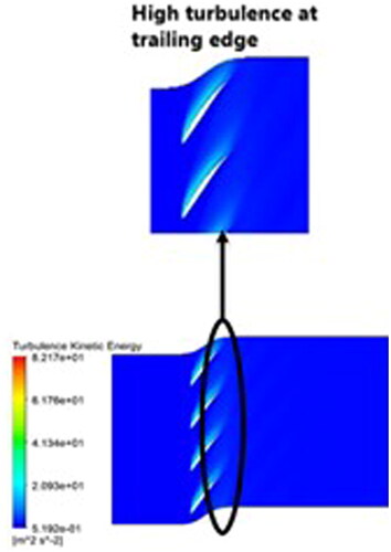
Figure 22. Turbulence kinetic energy distribution at injection baseline case.

5. Conclusions and future work

The axial flow compressor rotor blade NACA 65 is a low-speed compressor where flow control techniques would suppress the stall. Through tip injection, the aerodynamic losses are resolved, and the improvement is seen in the performance of the blade. The main conclusions of the current research work are noted below:

• Performance of an axial flow compressor rotor blade NACA 65 is analyzed using numerical simulation and validated with the experimental data and ensure behavior of the blade, an Active flow control technique is used to overcome the flow blockage which negatively impacts the performance.

• Grid independency tests have been examined for different number of mesh elements, and the optimal grid resolution is identified to balance accuracy and computational cost. For further simulation, 0.5 million mesh elements are fixed which convinces consistency in simulation.

• The numerical simulations are being examined for various turbulence models K-epsilon, K-omega, Generalize K-omega, shear stress transport and RNG K-epsilon, to assess the accuracy and reliability in predicting a convenient flow model. After validating the K-epsilon flow model, it is finalized and used for further simulation because it demonstrates good agreement with experimental data.

• Tip injection method is implemented upon the blade passage due to the formation of vortex breakdown and flow blockage near the tip and become unstable, it is an effective method for suppressing the instability in the compressor. Surprisingly, a small percentage of 0.3% injection gives a higher value of SMI.

• Effect of 0.3% injection mass flow and negative yaw angle SMI results in preferable performance than positive yaw angle.

The study concentrates on how tip injection positively impacts performance and stability. It recognizes that parameters, such as mass flow rate, pitch angle and change in yaw angle influence flow control and improvement in stall margin. Further study deals with the combination of Groove casing and tip injection to determine the effective behavior of the axial compressor.

Authors contributions

Prithesh Pinto: conceptualization, formal analysis, data curation, methodology, investigation and writing the original draft.

Srinivas G: conceptualization, supervision, data curation and report editing.

Acknowledgments

I want to express my deepest gratitude to the Director of Manipal Institute of Technology for your exceptional leadership and dedication toward the wellbeing of the institute. Under your leadership, our institution has flourished and grown in remarkable ways. I wholeheartedly thank Dr. Dayanad Pai, Head of the Department of Aeronautical and Automobile Engineering, for his culture of excellence and continuous growth. Your visionary approach has been instrumental in guiding us toward achieving our collective goal and reaching new heights. I am confident that the knowledge and skills I have acquired will have good impact on my future endeavors.

Disclosure statement

The author hereby declares there is no conflict of interest.

Data availability statement

The data that support the findings of this study are available from the author, Prithesh Pinto, upon reasonable request. For any inquiries regarding the data used in this study, please contact at [email protected].

Additional information

Funding

There are no investments for this research.

Notes on contributors

Prithesh Pinto

Prithesh Printo is an undergraduate student in aeronautical engineering. His areas of interest include aerodynamics, turbomachinery aerodynamics, propulsion, and CFD. He is passionate about advancing his knowledge and skills in these fields.

Srinivas G

Dr. Srinivas G. is an Associate Professor in the Department of Aeronautical and Automobile Engineering at Manipal Institute of Technology-MAHE, Manipal, Karnataka, India. He earned his bachelor’s degree in aeronautical engineering, his master’s degree in aerospace engineering, and his Doctor of Philosophy in the field of aircraft engine propulsion. His areas of interest include turbomachinery aerodynamics, aircraft propulsion, rocket propulsion, computational aerodynamics, and vehicle aerodynamics.

References

- Ahmad, N., Zheng, Q., Fawzy, H., Jiang, B., & Ahmed, S. A. (2020). Performance improvement of axial compressor by introduction of circumferential grooves. Energy Sources, Part A: Recovery, Utilization and Environmental Effects, 1, 1–21. https://doi.org/10.1080/15567036.2020.1756540
- Chen, H., Huang, X., Shi, K., Fu, S., Ross, M., Bennington, M. A., Cameron, J. D., Morris, S. C., McNulty, S., & Wadia, A. (2013). A computational fluid dynamics study of circumferential groove casing treatment in a transonic axial compressor. Journal of Turbomachinery, 136(3), 031003. https://doi.org/10.1115/1.4024651
- Duc Vo, H., Tan, C. S., & Greitzer, E. M. (2008). Criteria for spike initiated rotating stall. Journal of Turbomachinery, 130(1), 011023. https://doi.org/10.1115/1.2750674
- Epstein, A. H., Ffowcs Williams, J. E., & Greitzer, E. M. (1989). Active suppression of aerodynamic instabilities in turbomachines. Journal of Propulsion and Power, 5(2), 204–211. https://doi.org/10.2514/3.23137
- Fukuhara, M. (1985). M. inoue IVI. Kuroumaru behavior of tip leakage flow behind an axial compressor rotor. http://www.asme.org/about-asme/terms-of-use
- Gourdain, N., Burguburu, S., Leboeuf, F., & Miton, H. (2006). Numerical simulation of rotating stall in a subsonic compressor. Aerospace Science and Technology, 10(1), 9–18. https://doi.org/10.1016/j.ast.2005.07.006
- Hiller, S. J., Matzgeller, R., & Horn, W. (2011). Stability enhancement of a multistage compressor by air injection. Journal of Turbomachinery, 133(3), 031009. https://doi.org/10.1115/1.4001228
- Khaleghi, H. (2015). Stall inception and control in a transonic fan, part B: Stall control by discrete endwall injection. Aerospace Science and Technology, 41, 151–157. https://doi.org/10.1016/j.ast.2014.12.022
- Khaleghi, H., Dehkordi, M. A. S., & Tousi, A. M. (2016). Role of tip injection in desensitizing the compressor to the tip clearance size. Aerospace Science and Technology, 52, 10–17. https://doi.org/10.1016/j.ast.2016.02.003
- Kim, J. H., Choi, K. J., & Kim, K. Y. (2013). Aerodynamic analysis and optimization of a transonic axial compressor with casing grooves to improve operating stability. Aerospace Science and Technology, 29(1), 81–91. https://doi.org/10.1016/j.ast.2013.01.010
- Lu, X., Chu, W., Zhu, J., & Tong, Z. (2006). Numerical and experimental investigations of steady micro-tip injection on a subsonic axial-flow compressor rotor. International Journal of Rotating Machinery, 2006(1), 1–11. https://doi.org/10.1155/IJRM/2006/71034
- Nie, C., Xu, G., Cheng, X., & Chen, J. (2002). Micro air injection and its unsteady response in a low-speed axial compressor. Journal of Turbomachinery, 124(4), 572–579. https://doi.org/10.1115/1.1508383
- Shi, K., Chen, H. X., & Fu, S. (2013). Numerical investigation of the casing treatment mechanism with a single circumferential groove. Science China Physics, Mechanics and Astronomy, 56(2), 353–365. https://doi.org/10.1007/s11433-013-5003-y
- Srinivas, G., Raghunandana, K., & Satish, S. B. (2018). Axial-flow compressor analysis under distorted phenomena at transonic flow conditions. Cogent Engineering, 5(1), 1526458. https://doi.org/10.1080/23311916.2018.1526458
- Taghavi-Zenouz, R., & Ababaf Behbahani, M. H. (2018). Improvement of aerodynamic performance of a low speed axial compressor rotor blade row through air injection. Aerospace Science and Technology, 72, 409–417. https://doi.org/10.1016/j.ast.2017.11.028
- Vasudeva, V., Kumaraswamy, R. A., Kalra, S., & Saxena, A. (2021). Smart Innovation, Systems and Technologies 239. http://www.springer.com/series/8767
- Weichert, S., & Day, I. (2013). Detailed measurements of spike formation in an axial compressor. Journal of Turbomachinery, 136(5) https://doi.org/10.1115/1.4025166
- Wojewodka, M. M., White, C., Shahpar, S., & Kontis, K. (2018). A review of flow control techniques and optimisation in s-shaped ducts. In International Journal of Heat and Fluid Flow, 74, 223–235. https://doi.org/10.1016/j.ijheatfluidflow.2018.06.016