Effect of oil price on Nigeria’s food price volatility

Abstract

This study examines the effect of oil price on the volatility of food price in Nigeria. It specifically considers the long-run, short-run, and causal relationship between these variables. Annual data on oil price and individual prices of maize, rice, sorghum, soya beans, and wheat spanning from 2000 to 2013 were used. The price volatility for each crop was obtained using Generalized Autoregressive Conditional Heteroskedascity (GARCH (1, 1)) model. Our measure of oil price is the Refiner acquisition cost of imported crude oil. The Augmented Dickey–Fuller and Phillip–Perron unit root tests show that all the variables are integrated of order one, I (1). Therefore, we use the Johansen co-integration test to examine the long-run relationship. Our results show that there is no long-run relationship between oil price and any of the individual food price volatility. Thus, we implement a VAR instead of a VECM to investigate the short-run relationship. The VAR model result revealed a positive and significant short-run relationship between oil price and each of the selected food price volatility with exception of that of rice and wheat price volatility. These results were further confirmed by the impulse response functions. The Granger causality test result indicates a unidirectional causality from oil price to maize, soya bean, and sorghum price volatilities but does not show such relationship for rice and wheat price volatilities. We draw some policy implications of these findings.

Keywords:

• food price volatility
• world oil price
• co-integration
• VAR model
• Granger causality

Public Interest Statement

The food price hikes and spikes in recent times have raised concern among consumers and policy-makers. Crude oil price may have contributed to it. Oil is an important input in the production process. For instance, oil is used in manufacturing of fertilizer and other chemicals used in agricultural production process. Oil is also used to fuel farm machinery and to transport inputs and outputs. Hence, increases in the price of oil may add to production and distribution costs. Further, the use of biofuel as an alternative to petroleum may affect food price. This is because these biofuels are made from corn, soya beans, and other oilseeds. Therefore, an increase in the demand for these may affect the production, price level, and volatility of these crops and other food crops due to competition for fixed land. We empirically examine the link between oil price and volatility of selected food prices in Nigeria.

Competing interests

The authors declare no competing interest.

1. Introduction

Volatility is not new in agricultural market; however, since 2007, the degree of price volatility and the number of countries affected have been very high (High Level Panel of Experts, 2011). Food price volatility over the last four years has hurt millions of people, undermining nutritional status and food security (High Level Panel of Experts, 2011). Volatility is the rate of price variation over a successive period of time; it is determined by the speed, magnitude, and change in direction of the variation in prices (ECLAC/FAO/IICA, 2011). Volatility in the prices of agricultural raw materials can have serious consequences for countries: losses in economic efficiency, increased food insecurity, more malnutrition, negative impacts on their trade balance, possible social unrest to mention but a few (ECLAC/FAO/IICA, 2011). It is also feared to have a ravaging impact on the poor as greater percentage of their family budget is spent on food. This is why the issue of price volatility should be addressed to ameliorate the food insecurity situation in Nigeria.

Nigeria is an exporting and importing country in terms of crude oil and its products, respectively. Crude oil is arguably one of the most important driving forces of the Nigerian economy and changes in the price of oil would have significant effects on economic growth and welfare in Nigeria. Oil is used to power agricultural machines, processing machines, and to transport inputs such as fertilizer, pesticides, and final goods to the ultimate consumer. Increases in the price of oil therefore add serious pressure on the cost of these operations. Higher prices of oil may trigger inflation in the economy, increase cost of input, transport cost and subsequently reduce investment (Interagency Agency, 2011).

Gogoi (2014) investigated the long-run relationship between crude oil and world food commodity prices such as maize, rice, soybean, and wheat for the period between 1980 and 2011 using time series econometric technique. The co-integration test revealed that there is a long-run relationship between crude oil prices and the prices of maize, soybean, and wheat with the exception of rice prices. He also conducted a Granger causality test to check whether causality exists between the two prices. He found that there is unidirectional causality, with only crude oil prices “Granger causing” each of the four food commodity prices, while crude oil prices were not found to be influenced by price of food commodities.

Alvalos (2013) investigated whether oil price Granger cause corn and soybeans prices using a VAR model on monthly prices from January 1986 to April 2006 using international prices. His findings showed that oil price shocks exhibited no predictive causality over corn and soybeans prices. Oil prices have a negative impact both in the long- and short-run price dynamics of the two food commodities.

Arshad and Abdel Hameed (2009) also investigated if there is a long-term relationship between petroleum and cereal prices using monthly data over the period of January 1980 to March 2008. The bivariate co-integration approach using the Engle–Granger two-stage estimation procedures was applied and the result revealed unidirectional long-run causality from petroleum price to cereal prices.

Campiche, Bryant, Richardson, and Outlaw (2007) examined petroleum prices and global agricultural commodities prices. Their aim was to analyze the co-variability between crude oil prices and commodities such as corn, sorghum, sugar, soybeans, soybean oil, and palm oil. Using weekly data for the period of 2003–2007, they investigated the co-integration (i.e. long run) relationship between the variables using Johansen co-integration test. The Johansen co-integration test carried out for the period of 2003–2005 and 2006–2007 revealed a co-integration of corn and soybean prices with crude oil but only during 2006–2007.

However, some studies found no relationship between crude oil price and agricultural commodity prices. For instance, Esmaeili and Shokoohi (2011) found no direct long-run relationship between oil prices and agricultural commodity prices. Yu, Bessler, and Fuller (2006) examined the long-run relationship between crude oil prices and the prices of vegetable oils (oil palm, soybeans, rape seeds, sunflower) and found that crude oil price have no effect on vegetables oils prices. Apart from using international food prices, the papers reviewed above worked on oil price and selected food crop price not food price volatility.

Huchet-Bourdon (2011) statistically analysed the historical commodity price volatility over the last half century for an extended range of agricultural commodities such as beef, maize butter, rice, soybean oil, sugar, wheat, and whole milk. The paper also investigated the relationship between oil price, fertilizer price, and each of these agricultural commodities; however, using spearman’s correlation coefficient on monthly data which can only indicate the existence of a relationship but cannot indicate which one has a predictive power on the other.

Also, Ano Sujithan, Avouyi-Dovi, and Kolia (2014) used Bayesian multivariate framework to assess the effect of oil price and other drivers on the volatility of global prices of cocoa, coffee, sugar, and wheat in recent periods. Using monthly data covering the period January 2001–March 2013, an impulse response function of food volatility to oil price shocks revealed that an oil price shock leads to an increase in the price volatility of cocoa, coffee, sugar, and wheat for 2–3 months followed by a downward peak after 4 months. The result showed a negative impact on the volatility of soybeans and sugar and a positive impact on cocoa, coffee, corn, and wheat prices.

Although, Huchet-Bourdon (2011) and Ano Sujithan et al. (2014) worked on oil price and food price volatility, apart from using international food prices, their methodology is different. This is why this study used Johansen co-integration, VECM/VAR model, and the standard Granger causality test to analyse the effect of oil price on selected crops using domestic food price volatility. Specifically, the study examines the long- and short-run relationship between these variables as well as the causal relationship between them.

2. Methology

2.1. Data

The study used time series data which are secondary data type. Annual data on oil price (Refiner Acquisition Cost of Imported Crude Oil) were obtained from the US Energy Information Administration (EIA) from 2000 to 2013, and annual data on selected food crop prices were also sourced from Federal Ministry of Agriculture from 2000 to 2013. Then, the price volatility of each crop was estimated using GARCH (1, 1) model.

2.2. Econometric methodology

In this study, data were analyzed using descriptive and inferential statistics. Graphs were used to describe the trend or movement of price volatility of these crops and oil prices from 2000 to 2013. To check for the stationarity or non-stationarity of the series, the Augmented Dickey–Fuller and Phillip–Perron tests were used. The Johansen (1991, 1995) co-integration test was used to examine the long-run relationship, while the VAR model was used to determine the short-run relationship. The use of the VAR model was based on the outcome of the co-integration result. Lastly, the standard Granger causality was used to check if oil price has a predictive power on the food crop volatility.

2.3. Unit root test

Unit root tests were carried out to establish whether or not each series is stationary. It is important to test for the presence of unit root in time series to avoid the problem of spurious regression as described by Granger and Newbold (1974) cited by Gogoi (2014). If unit root is found, then the conditions of stationarity are violated. The most commonly used test is the Augmented Dickey–Fuller test (ADF). The test equation for food price volatility and oil price are given as:(1) $$\text{Maize:}\mathrm{\Delta }{\text{MPVOL}}_t={\mathit{\alpha }}_0+{\mathit{\alpha }}_{1}t+\mathit{\beta }{\text{MPVOL}}_{t-1}+\sum _{i=1}^p{\mathit{\delta }}_i\mathrm{\Delta }{\text{MPVOL}}_{t-i}+{\mathit{\epsilon }}_t$$(1) (2) $$\text{Rice:}\mathrm{\Delta }{\text{RPVOL}}_t={\mathit{\alpha }}_0+{\mathit{\alpha }}_{1}t+\mathit{\beta }{\text{RPVOL}}_{t-1}+\sum _{i=1}^p{\mathit{\delta }}_i\mathrm{\Delta }{\text{RPVOL}}_{t-i}+{\mathit{\epsilon }}_t$$(2) (3) $$\text{Sorghum:}\mathrm{\Delta }{\text{SPVOL}}_t={\mathit{\alpha }}_0+{\mathit{\alpha }}_{1}t+\mathit{\beta }{\text{SPVOL}}_{t-1}+\sum _{i=1}^p{\mathit{\delta }}_i\mathrm{\Delta }{\text{SPVOL}}_{t-i}+{\mathit{\epsilon }}_t$$(3) (4) $$\text{Soyabean:}\mathrm{\Delta }{\text{SOYPVOL}}_t={\mathit{\alpha }}_0+{\mathit{\alpha }}_{1}t+\mathit{\beta }{\text{SOYPVOL}}_{t-1}+\sum _{i=1}^p{\mathit{\delta }}_i\mathrm{\Delta }{\text{SOYPVOL}}_{t-i}+{\mathit{\epsilon }}_t$$(4) (5) $$\text{Wheat:}\mathrm{\Delta }{\text{WPVOL}}_t={\mathit{\alpha }}_0+{\mathit{\alpha }}_{1}t+\mathit{\beta }{\text{WPVOL}}_{t-1}+\sum _{i=1}^p{\mathit{\delta }}_i\mathrm{\Delta }{\text{WPVOL}}_{t-i}+{\mathit{\epsilon }}_t$$(5) (6) $$\mathrm{\Delta }{\text{OILP}}_t={\mathit{\alpha }}_0+{\mathit{\alpha }}_{1}t+\mathit{\beta }{\text{OILP}}_{t-1}+\sum _{i=1}^p{\mathit{\delta }}_i\mathrm{\Delta }{\text{OILP}}_{t-i}+{\mathit{\epsilon }}_t$$(6)

where MPVOL, RPVOL, SOYAPVOL, SPVOL, and WPVOL is the price volatility for maize, rice, soya bean, sorghum, and wheat, respectively, while OILP represents oil price, α₀ is the constant, α₁ is the coefficient of the trend series, p is the lag order of the autoregressive process for each food price e.g. ${\text{MPVOL}}_{t-1}$ is lagged value of order one of ${\text{MPVOL}}_{t-1}$ and ɛ_t is the error term. Dickey–Fuller adds lagged dependent variables to the test equation to remove distortions to the level of statistical significance but lowers the power of the test to detect a unit root when one is present. The null hypothesis can be evaluated by testing whether β = 0, while the alternative hypothesis tests whether β ≠ 0. A rejection of the null hypothesis implies that the series is stationary.

2.4. Co-integration test

According to Engle and Granger (1987), two series integrated of the same order I (q) are said to be co-integrated, if the linear combination of the two variables generate a stationary series. A non-stationary series that is co-integrated may diverge in the short run, but must be linked together in the long run. The co-integrated variables will never move far apart, and will be attracted to their long-run relationship (Koop, 2000). Testing for co-integration implies testing for the existence of such a long-run relationship between economic variables.

Although there are different ways of testing for co-integrations between variables, for the purpose of this study the Johansen co-integration test was used to determine the long-run relationship between food commodity price volatility and oil price. It is superior to other tests and has all desirable statistical properties. It is capable of determining the number of co-integrating relations among variables. Its weakness is that it relies on asymptotic properties and is therefore sensitive to specification. According to this technique, to determine whether two variables are co-integrated, we first have to ascertain the order of integration of the variables that are being modeled. This pre-testing is done by the unit root test as earlier discussed. To proceed with co-integration test in the Johansen framework, the two variables have to be integrated of the same order. If we establish that two variables are integrated of the same order, then we proceed next to estimate the long-run equilibrium relationship. The Johansen test is a VAR-based co-integration test. Consider a general VAR of order p:(7) $$y_t=A_1{y}_{t-1}+....+A_p{y}_{t-p}+Bx{t}_{t-i}+{\mathit{\epsilon }}_t$$(7)

where y_t is a k-vector of non-stationary variables that are for instance integrated of order 1 and commonly denoted as I (1). In this study, y_t consists of oil price and each of the food commodity price, taking OILP_t and MPVOL_t for instance, x_t is a d-vector of deterministic or exogenous variables which are optional, and ɛ_t is a vector of innovations or random shocks. The VAR may be rewritten as:(8) $$\mathrm{\Delta }{y}_t=\mathit{\Pi }{y}_{t-1}+\sum _{i=1}^{p-1}{\mathrm{\Gamma }}_i\mathrm{\Delta }{y}_{t-i}+B{x}_t+{\mathit{\epsilon }}_t$$(8)

where(9) $$\mathit{\Pi }=\sum _{i=1}^p{A}_i-I,{\mathrm{\Gamma }}_i=-\sum _{j=i+1}^p{A}_j$$(9)

Granger’s representation asserts that if the coefficient matrix Π has reduced rank r < k, then there exist matrices α and β each with a rank r such that Π = αβ^′ and β^′y_t is I (0). r is the number of co-integrating relationships (i.e. the co-integrating rank) and each column of β is the co-integrating vector. The elements of α are known as the adjustment parameters in the VEC model. Johansen’s method is to estimate the Π matrix from an unrestricted VAR and to test whether we can reject the restrictions implied by the reduced rank of Π. It can be shown that for a given r, the maximum likelihood estimator of β defines the combination of y_t − 1 that yields the r largest canonical correlations of Δy_t with y_t − 1 after correcting for lagged differences and deterministic variables when present. For this study, deterministic or exogenous variables such as seasonal dummies or time trends are not included. Johansen proposes two different likelihood ratio tests of the significance of these canonical correlations and thereby the reduced rank of the Π matrix: the trace test and maximum eigenvalue test. The trace test tests the null hypothesis of r co-integrating vectors against the alternative hypothesis of k co-integrating vectors. The maximum eigenvalue test, on the other hand, tests the null hypothesis of r co-integrating vectors against the alternative hypothesis of r + 1 co-integrating vectors. If the variables OILP and MPVOL are not co-integrated, the analysis will proceed in a VAR framework. The empirical model is then specified as:(10) $$\begin{array}{c}{\text{OILP}}_t={\mathit{\delta }}_0+\sum _{i=1}^p{\mathit{\varphi }}_i{\text{OILP}}_{t-i}+\sum _{i=1}^p{\mathit{\gamma }}_i{\text{MPVOL}}_{t-i}+{\mathit{\epsilon }}_{1,t}\\ {\text{MPVOL}}_t={\mathit{\eta }}_0+\sum _{i=1}^p{\mathit{\lambda }}_i{\text{OILP}}_{t-i}+\sum _{i=1}^p{\mathit{\theta }}_i{\text{MPVOL}}_{t-i}+{\mathit{\epsilon }}_{2,t}\end{array}$$(10)

The formulations above apply irrespective of the particular food price volatility that is being considered.

Only the variable names and notations changes.

2.5. Causality test

Granger causality measures the precedence or information content or the predictability of the past values of one variable for the current values of another variable. According to Granger (1969) causality, if a series Y₁ “Granger-causes” a series Y₂, then past values of Y₁ should contain information that helps predict Y₂ above and beyond the information contained in past values of Y₂ alone. Its mathematical formulation is based on linear regression modeling of stochastic processes.

The basic Granger causality definition is quite simple. If we have two time series OILP_t and MPVOL_t for instance and we attempt to forecast MPVOL_t using past terms of OILP_t. Then, OILP_t is said to “Granger cause” MPVOL_t if OILP_t helps in the prediction of MPVOL_t. The definition leans on the idea that cause occurs before the effect and this is the basis of most all causality definitions. It could be, also must be, a two-way causality that is if OILP_t causes MPVOL_t and MPVOL_t causes OILP_t.

The causality relationship can be evaluated by estimating the following linear regression models. Consider a bivariate linear autoregressive model of the two variables OILP_t and MPVOL_t. The important thing to point out here is that if the variables have a trend, then it is most likely to show that there is correlation between them. However, in general, correlation does not mean causation. The empirical bivariate regression model for the case of oil price and maize price volatility (MPVOL) is specified as:(11) $$\begin{array}{c}{\text{OILP}}_t={\mathit{\delta }}_1+\sum _{i=1}^p{\mathit{\varphi }}_{11,i}{\text{OILP}}_{t-i}+\sum _{i=1}^p{\mathit{\varphi }}_{12,i}{\text{MPVOL}}_{t-i}+{\mathit{\epsilon }}_{1,t}\\ {\text{MPVOL}}_t={\mathit{\delta }}_2+\sum _{i=1}^p{\mathit{\varphi }}_{21,i}{\text{OILP}}_{t-i}+\sum _{i=1}^p{\mathit{\varphi }}_{22,i}{\text{MPVOL}}_{t-i}+{\mathit{\epsilon }}_{2,t}\\ \end{array}$$(11)

Here p is the number of lagged observations included in this model which were determined using the Akaike information criteria (AIC) (Akaike, 1974) and the Schwartz information criteria (SIC) (Schwarz, 1978); the matrix φ contains the coefficients of the model; ɛ₁, and ɛ₂, are residuals (prediction errors) for each time series. Again, similar formulation applies to the other food commodity prices.

According to Gogoi (2014), if the variance of ɛ₁, or ɛ₂, is reduced by the inclusion of MPVOL or OILP terms in the first or second equation, then it is said that MPVOL or OILP Granger causes OILP or MPVOL. In other words, OILP Granger causes MPVOL if the coefficients in φ_21,i are jointly significantly different from zero. This can be tested by performing an F-test of the null hypothesis that φ_21,i = 0, given assumptions of covariance stationarity on OILP and MPVOL. Analogously, MPVOL Granger causes OILP if the coefficients in φ_12,i are jointly significantly different from zero. This can be tested by performing an F-test of the null hypothesis that φ_12,i = 0. The hypothesis is as following:

H₀: OILP_t (or MPVOL) does not cause MPVOL (or OILP_t)

H₁: OILP_t (or MPVOL) cause MPVOL (or OILP_t)

The null hypothesis would be rejected for a small p-value (p ≤ 0.1). This implies that there is causation. If the null cannot be rejected then it means that there is no causal relationship between the variables. In other words, the two variables have no predictive or information content for each other.

3. Results and discussion

3.1. The trend of variables used

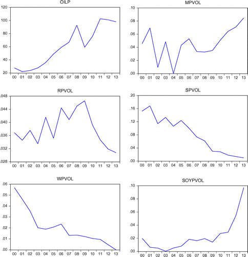
Figure 1 shows the trend of the oil price and food price volatility. The trend in oil price (OILP) shows a constant increase in oil price from about US$27 per barrel in the year 2000 to a high of about US$92 per barrel in the year 2008. This movement dropped in the year 2009 and started increasing in the year 2010 and peaked at US$102 per barrel in 2011. As at 2013, it stood at about US$ 98 per barrel. The selected food price volatility measures the variability in the relative price of a specific crop. For each crop, the indicator is calculated from the annual crop price level. The GARCH (1, 1) model was used to estimate the selected food price volatilities. The data span from 2000 to 2013. It was observed that each selected crop exhibits some levels of volatility.

Figure 1. Trend of World oil price and Nigeria food price volatility.

3.2. Unit root tests

The ADF and Philip–Perron (PP) unit root tests were used to check for stationarity or non-stationarity of variables as described in the methodology. The results for all the variables are presented in Table 1. A decision can be taken based on either the t-statistics or p-values (probability). Both the ADF and PP tests results indicate that all selected food crop volatilities have unit roots and therefore non-stationary in levels.

Table 1. ADF and PP test^a

Variables	Level		First difference		Decision
	t-statistic	Probability	t-statistic	Probability
ADF
OILP	−0.765	0.795	−4.177^***	0.010	I (1)
MPVOL	−0.768	0.791	−7.151^***	0.000	I (1)
RPVOL	−1.564	0.466	−5.528^***	0.001	I (1)
SPVOL	−1.027	0.707	−8.077^***	0.000	I (1)
SOYPVOL	−1.562	0.903	−8.104^***	0.000	I (1)
WPVOL	2.258	0.910	−4.354^***	0.008	I (1)
PP
OILP	−0.178	0.920	−8.500^***	0.000	I (1)
MPVOL	−2.657^***	0.107	−7.151^***	0.000	I (1)
RPVOL	−1.858^**	0.339	−5.133^***	0.002	I (1)
SPVOL	−0.478	0.867	−8.077^***	0.000	I (1)
SOYPVOL	−1.513	0.496	−5.551^***	0.001	I (1)
WPVOL	−2.258^***	0.999	−5.747^***	0.001	I (1)

^*** Significance at 1% level.

^** Significance at 5% level.

However, for all variables, the null hypothesis of unit root is rejected by both ADF and PP unit root tests at 1% level when we conduct the analysis on their first differences. This implies that maize, rice, soya bean, wheat, and sorghum volatilities and world oil price have no unit roots (i.e. stationary) in their first differences and are therefore integrated of order one, I (1).

3.3. Long-run analysis

The Johansen co-integration test was used to check for any long-run relationship between oil price and the price volatilities of maize, rice, wheat, soya bean, and sorghum. The results are presented in Table 2. The results from both the maximum eigenvalue and trace test show that there is no co-integration between oil price and the individual crop price volatilities as the 5% critical value (CV) is greater than the test statistics in all cases. This implies that there is no long-run relationship between oil price and the price volatilities of maize, rice, wheat, soya bean, and sorghum. The absence of co-integration implies that the price of oil and individual food prices do not follow the same long-run trend. They do not co-move with each other over time. Therefore, it can be said the linear combination of the oil price and each of the food price volatility is not stationary. The absence of long-run relationship also implies that if these variables deviate from the mean or equilibrium level, it will be difficult to bring them back to equilibrium, since there is no error correction for the relationship. As a result, the price of oil might drift above or below the individual food prices in the long run. However, this does not preclude the possibility of sharing a significant relationship in the short term. We therefore proceed to determine the short-run relationship between the individual price volatilities and oil price in the next section using the VAR instead of the VECM.

Table 2. Johansen co-integration test

Trace test				Maximum eigenvalue test
H0	H1	Statistic	5% CV	H0	H1	Statistic	5% CV
Co-integration test between OILP and MAIZPVOL
r = 0	r ≥ 1	10.115	15.494	r = 0	r = 1	9.715	14.265
r ≤ 1	r ≥ 2	0.400	3.841	r = 1	r = 2	0.400	3.841
Co-integration test between OILP and RPVOL
r = 0	r ≥ 1	7.360	15.495	r = 0	r = 1	6.399	14.264
r ≤ 1	r ≥ 2	0.960	3.841	r = 1	r = 2	0.960	3.841
Co-integration test between OILP and WPVOL
r = 0	r ≥ 1	13.174	15.495	r = 0	r = 1	12.229	14.265
r ≤ 1	r ≥ 2	0.944	3.841	r = 1	r = 2	0.944	3.841
Co-integration test between OILP and SPVOL
r = 0	r ≥ 1	12.114	15.495	r = 0	r = 1	11.279	14.265
r ≤ 1	r ≥ 2	0.835	3.841	r = 1	r = 2	0.835	3.841
Co-integration test between OILP and SOYPVOL
r = 0	r ≥ 1	14.99	15.495	r = 0	r = 1	11.824	14.264
r ≤ 1	r ≥ 2	3.167	3.841	r = 1	r = 2	3.167	3.841

3.4. Short-run analysis

Since there was no co-integration between oil price and individual food price volatilities, vector autoregressive model (VAR) was estimated. We present both the estimates and the impulse response functions to describe the short-run relationship between oil price and the price volatility of the five food crops under study. The result on the VAR estimates is presented in Table 3. The R² value for each of the bivariate VAR models indicates that the overall goodness of fit of the VAR is satisfactory. For instance, 74.7% of the variation in MVOL is explained by oil price. The remaining 25.3% is inherent in the error term. The F-statistic shows the joint significance of all the variables in determining the individual price volatility in each case.

Table 3. VAR estimates between OILP and individual food price volatility

Bivariate VAR estimates of oil price and maize price volatility
	OILP			MPVOL
	Coeff.	S.E	t-stat	Coeff.	S.E	t-stat
OILP (−1)	0.890^***	0.175	5.093	0.001^**	0.0002	1.963
MPVOL (−1)	−29.82	242.3	−0.123	−0.103	0.328	−0.314
Constant	13.011	12.324	1.056	0.024	0.0167	1.425
R^2	0.747			2.881
F-statistic	14.762			2.024
Bivariate VAR estimates of oil price and rice price volatility
	OILP			RPVOL
	Coeff.	S.E	t-stat	Coeff.	S.E	t-stat
OILP (−1)	0.880^***	0.163	5.396	−1.78E	5.0E	−0.354
RPVOL (−1)	169.87	1,003.8	0.169	0.492	0.311	1.582
Constant	5.779	39.26	0.147	14.773	7.969^*	1.854
R^2	0.747			0.203
F-statistic	14.79			1.272
Bivariate VAR estimates of oil price and sorghum price volatility
	OILP			SPVOL
	Coeff.	S.E	t-stat	Coeff.	S.E	t-stat
OILP (−1)	0.785^***	0.222	3.523	0.429^**	0.199	2.153
SPVOL (−1)	−0.102	0.147	−0.696	0.858^***	0.132	6.495
Constant	0.661	0.587	1.125	1.084	0.527	2.057
R^2	0.845			0.957
F-statistic	27.21			111.9
Bivariate VAR estimates of oil price and soya bean price volatility
	OILP			SOYPVOL
	Coeff.	S.E	t-stat	Coeff.	S.E	t-stat
OILP (−1)	1.015^***	0.161	6.294	2.215^***	0.688	3.219
SOYPVOL (−1)	−0.062	0.064	−0.966	−0.017	0.274	−0.068
Constant	−0.247	0.855	−0.289	−13.187^***	−3.647	−3.615
R^2	0.851				0.639
F-statistic	28.59				0.567
Bivariate VAR estimates of oil price and wheat price volatility
	OILP			WPVOL
	Coeff.	S.E	t-stat	Coeff.	S.E	t-stat
OILP (−1)	0.540^**	0.210	2.564	−7.66E-05	6.8E-05	−1.130
WPVOL (−1)	−850.897^**	401.799	−2.118	0.648	0.129^***	5.009
Constant	50.389^**	19.986	2.521	0.008	0.006	1.203
R^2	0.825			0.895
F-statistic	23.581			42.640

^* Significant at 10% level.

^** Significance at 5% level.

^*** Significance at 1% level.

Results show that world oil price has a positive short-run effect on MPVOL, soya beans price volatility (SOYPVOL), and sorghum price volatility (SPVOL). For MPVOL and SOYPVOL the effect is significant at 5%, while it is significant at 1% for SPVOL. However, OILP has a negative short-run effect on rice price volatility (RPVOL) and wheat price volatility (WPVOL) though these are not significant at any conventional levels. The puzzle observed for rice and wheat may be due to the fact that these two are mainly imported food staples (Nigeria INTEL, 2012). Hence, it is possible that the effect of oil price on rice and wheat could have been better captured by accounting for exchange rate effects.

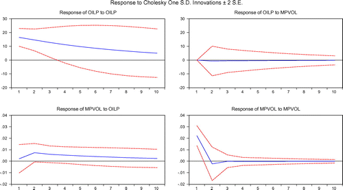
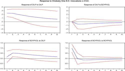
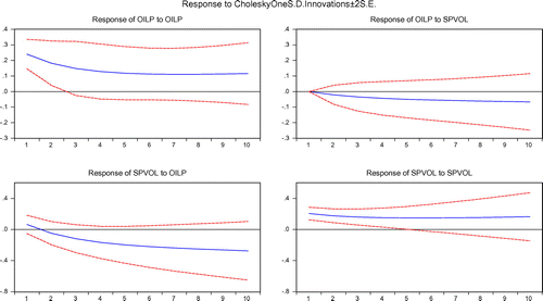
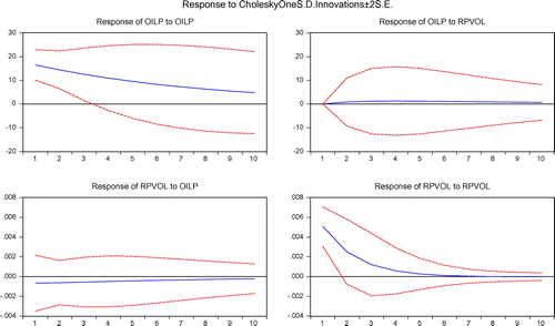
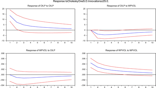
Further evidence of the short-run relationship between the variables can be inferred from the impulse responses. The impulse responses of the selected food price volatilities to a shock in oil price are presented in Figures 2–6. From Figure 2, the response of MPVOL to a positive shock in oil price is positive and persistent throughout the entire period but this is not significant at any time. This is consistent with Ano Sujithan et al. (2014) whose research revealed a positive impulse response of international MPVOL to a shock in oil price. The response of RPVOL in Figure 3 was persistently negative but insignificant. The response of soya bean as shown in Figure 4 is positive throughout and significant between the second and the fourth period. For sorghum as depicted in Figure 5, its response is positive between the first and second period before turning to negative and remained negative to the end but insignificant. WPVOL’s response as shown in Figure 6 was persistently negative but insignificant. This result is not consistent with Ano Sujithan et al. (2014), as his findings showed that international WPVOL responded positively to a shock in oil price. However, this is not to be worried about since the response though negative is not significant.

Figure 2. Impulse response function between oil price and MPVOL.

Figure 3. Impulse response function between oil price and soya bean price volatility.

Figure 4. Impulse response function between oil price and SPVOL.

Figure 5. Impulse response function between oil price and RPVOL.

Figure 6. Impulse response function between oil price and WPVOL.

3.5. Granger causality

The Granger causality test is used to show if oil price has a predictive power on the selected food price volatility and vice versa. The Granger causality test results are presented in Table 4. The test performed on individual food price volatility indicates that a unidirectional causality runs from oil price to maize, soya bean, and sorghum price volatilities but not vice versa. The results are significant at 5% for maize and sorghum and at 1% for soya bean. The null hypothesis cannot be rejected for rice and wheat price volatilities. This implies that oil price can be used to predict maize, soya bean, and sorghum price volatilities but cannot be used to predict rice and wheat price volatilities.

Table 4. Granger causality analyses

Null hypothesis	χ^2	Prob.
OILP does not Granger cause MPVOL	3.852^**	0.049
MPVOL does not Granger cause OILP	0.015	0.902
OILP does not Granger cause RPVOL	0.125	0.724
RPVOL does not Granger cause OILP	0.029	0.882
OILP does not Granger cause SPVOL	4.633^**	0.031
SPVOL does not Granger cause OILP	0.484	0.334
OILP does not Granger cause SOYPVOL	10.359^***	0.001
SOYPVOL does not Granger cause OILP	0.933	0.334
OILP does not Granger cause WPVOL	0.739	0.691
WPVOL does not Granger cause OILP	1.422	0.491

^** Significance at 5% level.

^*** Significance at 1% level.

4. Conclusion and recommendation

In conclusion, the findings of this study show that there is no long-run relationship between oil price and any of the individual price volatilities as indicated by the Johansen co-integration test. However, in the short run, oil price had positive and significant effect on maize, soya bean, and SPVOL as indicated by the VAR estimates and supported by the impulse response functions. Oil price has a negative albeit insignificant effect on rice and wheat price Again, these are largely confirmed by the impulse response functions. The Granger causality test shows that there is a unidirectional causality running from oil price to maize, soya bean, and sorghum price volatilities. However, causality does not run from oil price to rice and wheat price volatilities. The reason for finding neither short-run nor causal relationship between oil price and wheat and rice could be deduced that Nigeria imports more of these crops than they produce (thetidenewsonline.com, 2013). Hence, further studies may deduced consider including exchange rate in examining such relationship.

Our results also show that agricultural commodity price has some degree of volatility inherent in them. Therefore, intervention in this regard is required to reduce its price variability to its natural level where it will not be a problem to the farmers or threaten the food security in the country. These interventions also could be relevant in times of food crisis. These include improvement in the market information system as this would reduce market speculations, price hikes, and uncertainty.

It is obvious from this study that oil shocks has a significant short-run effect on some of the food price volatility in Nigeria; therefore, recommendations to this regard will be geared towards ensuring that pump price of refined oil or crude oil products are being controlled, ensuring that the refineries are working at a maximum capacity, encouraging the use of alternative source of energy and organic fertilizer to cushion the effect of high oil prices on food prices.

Additional information

Funding

Funding. The authors received no direct funding for this research.

Notes on contributors

Ijeoma C. Nwoko

Ijeoma C. Nwoko obtained her MSc in Agricultural Economics from University of Agriculture Makurdi, Nigeria in 2015. She has the intention of advancing her research capabilities in by enrolling for her doctorate degree and creating both local and international networks. She has interest in energy and environmental economics.

Goodness C. Aye

Goodness C. Aye obtained her PhD in Agricultural Economics from University of Pretoria. She is a senior lecturer at University of Agriculture, Makurdi, Nigeria and has continued to maintain her research collaborations all over the world. Her several publications cover policy analysis, development economics, production economics, environmental economics, energy economics, and poverty studies.

Benjamin C. Asogwa

Benjamin C. Asogwa holds a PhD in Agricultural Economics. He is a senior lecturer in the Department of Agricultural Economics, University of Agriculture, Makurdi, Nigeria. His special research interests include: Production Economics, Agricultural Marketing, Agricultural Finance, Farm Management, Agribusiness, Agricultural Policy and Development Economics.

References

- Akaike, H. (1974). A new look at the statistical model identification. IEEE Transactions on Automatic Control, 19, 716–723.10.1109/TAC.1974.1100705
- Ano Sujithan, K., Avouyi-Dovi, S., & Kolia, L.. (2014). On the determinants of food price volatility. Paris: Dauphine University.
- Arshad, F. M., & Abdel Hameed, A. A. (2009). The long run relationship between petroleum and cereal prices. Global Economy and Finance Journal, 2, 91–100.
- Alvalos, F. (2013) Do oil prices drive food prices. In A Natural Experiment; Proceeding of the 6th International Conference on Economic Studies, July 22, 2011. Cartagena: Fondo Latinomericano de Reservas.
- Campiche, J., Bryant, H., Richardson, J., & Outlaw, J. (2007, July 29–August 1). Examining the evolving correspondence between petroleum prices and agricultural commodity prices. Paper presented at the American Agricultural Economics Association Annual Meeting, Portland, OR.
- Esmaeili, A., & Shokoohi, Z. (2011). Assessing the effect of oil price on world food prices: Application of principal component analysis. Energy Policy, 39, 1022–1025.10.1016/j.enpol.2010.11.004
- Engle, R. F., & Granger, C. W. J. (1987). Co-integration and error correction: Representation, estimation and testing. Econometrica, 55, 251–276.10.2307/1913236
- ECLAC/FAO/IICA. (2011). Price volatility in agricultural markets (2000–2010): Implication for Latin America for policy options. The outlook for agricultural and rural development in the Americas: A perspective on Latin American and the Caribbean. Santiago.
- Gogoi, A. (2014). Investigating the long run relationship between crude oil and food commodity prices ( MSc thesis). Department of Economics, University of Nottingham, Nottingham.
- Granger, C. W. J. (1969). Investigating causal relations by econometric models and cross-spectral methods. Econometrica, 37, 424–438.10.2307/1912791
- Granger, C. W. J., & Newbold, P. (1974). Spurious regression in econometrics. Nothingham: North-Holland.
- High Level Panel of Experts. (2011). Price volatility and food security. A Report by the High-Level Panel of Experts on Food Security and Nutrition Committee on World Food Security. Rome.
- Huchet-Bourdon, M. (2011). Agricultural commodity price volatility: An overview (OECD Food, Agriculture and Fisheries Papers, No. 52). Organization for Economic Cooperation Development. Paris: OECD.
- Interagency Report to the G20. (2011). Price volatility in food and agricultural markets: Policy responses. Policy Report including Contributions by FAO, IFAD, IMF, OECD, UNCTAD, WFP, World Bank, WTO, IFPRI and UMHTF.
- Johansen, S. (1991). Estimation and hypothesis testing of cointegration vectors in Gaussian vector autoregressive models. Econometrica, 59, 1551–1580.10.2307/2938278
- Johansen, S. (1995). Likelihood-based inference in cointegrated vector autoregressive models. Oxford: Oxford University Press.10.1093/0198774508.001.0001
- Koop, G. (2000). Analysis of economic data (pp. 153–154). University of Glasgow. Chichester, NY: Wiley.
- www.thetidenewsonline.com/nigeria. (2013, July 17). Nigeria spends N1.7trillion on food importation annually-Minister of Agriculture.
- Schwarz, G. E. (1978). Estimating the dimension of a model. The Annals of Statistics, 6, 461–464.10.1214/aos/1176344136
- Yu, T-H., Bessler, D. A., & Fuller, S. (2006, July 23–26). Cointegration and causality analysis of world vegetable oil prices. Paper Presented at American Agricultural Economics Association Annual Meeting. Long Beach, CA.