Application of ARIMA models in forecasting livestock products consumption in Tanzania

Abstract

Poverty is a major problem Tanzania is facing, which depends on agriculture as the main economic activity. Different stakeholders have involved themselves in boosting agricultural productivity, especially in semiarid regions, where their main focus is on drought tolerant crops such as sorghum and millet. If this support is not linked with market opportunities, commodity prices may be depressed and discourage farmers. This paper determines prospect for increasing utilization of animal feed as the market opportunity for farmer by forecast consumption of livestock product such as eggs, milk, chicken and cow meat. Autoregressive integrated moving average models were used for forecasting with the data from FAOSTAT. The result shows that consumption of all livestock products will increase, hence expected demand for animal feed. This paper calls for more research works in analyzing factors that may affect consumption of livestock products such as population increase and change of consumption behavior toward livestock products.

Keywords:

• livestock production
• ARIMA models
• sorghum and millet farming
• semiarid regions
• feed industry

PUBLIC INTEREST STATEMENT

Poverty is a major problem Tanzania is facing, which depends on agriculture as the main economic activity for more than 75% of the population. Different stakeholders have involved themselves in boosting agricultural production especially in regions with less rain. Their main focus is in crops that need less rainfall such as sorghum and millet. If this support is successful, production will increase; however, if this increase in production is not linked with the market, prices may drop and discourage farmers. This paper determines the possibility of future increasing in usage of livestock product as the market opportunity for farmer in regions with less rainfall. The result shows that consumption of all livestock products will increase in the next five years. This means that there is an opportunity of farmers in regions of less rainfall to cultivate crops such as sorghum and millet and sell them in animal feed.

Competing interests

The author declares no competing interests.

1. Introduction

Poverty is a major problem many African countries are facing, especially in the south of Sahara desert. Tanzania is one of the countries, with a population of about 45 million people (Tanzania, 2014). The main economic activity is agriculture which employs about 75% of the total population. Even though agriculture is the main activity, its structure is dominated by smallholder farmers who cultivate average farm size of .9–3 ha each with the use of very low technology. It is estimated that 70% of crop area is cultivated by hand hoe, 20% by ox plough and 10% by tractors (Chauvin, Mulangu, & Porto, 2012; Chauvin et al., 2012; Group, 2011; Majid, 2008). Due to poor technology and rainfall dependence system, the agricultural sector has shown poor performance and hence promotes more poverty to those who depend on it.

Both the government of Tanzania and other stakeholders have involved themselves in different projects to promote the generation and adoption of technologies that are capable of boosting agricultural productivity. In semiarid region, initiatives have been mainly focusing on drought-tolerant crops such as sorghum and millet rather than tropical crops such as maize, which requires a more even distribution of rainfall (Blum & Sullivan, 1986). This support of government and donors to crops like sorghum and millet is important in increasing agricultural productivity in semiarid regions. But these projects could depress commodity prices and farmers’ incomes if they are not linked to market opportunities for farmers, especially with the presence of preferred substitute crops such as maize (Amani, 2005).

Feed industry is a potential market for sorghum and millet to substitute maize in the market (Rohrbach and Kiriwaggulu, 2001). According to Abdulkadir, Na-Allah and Bala (2013) and Issa, Jarial, Brah, Harouna and Soumana (2015), sorghum can absolutely or partially replace maize in animal feed especially in poultry industry. As maize is preferred than sorghum and millet due to availability and price stability, linking farmers in feed industry is important. Substituting maize with sorghum and millet will be advantageous as it will eliminate competition between animals and humans in the consumption of maize. This paper estimates prospects for increasing utilization in feed concentrate market by forecast production of livestock product such as eggs, milk, chicken and cow meat.

2. Methodology

Autoregressive integrated moving average (ARIMA) models were used to forecast production of livestock products. These models were used because they consider only one variable under each observation. Scholars in different discipline such as Jose and Sojan (2013), Yeboah, Ohene and Wereko (2012), Wang and Yang (2017), Manoj and Madhu (2014),  Mandal (2005) and Raymond (1997) used these models for forecasting. The main assumption of these models is that in time series analysis, there is an aspect of past patterns, which continue to remain in the future (Ramasubramanian, 2001; Heng, Zhang, & Yang, 2017). These models capture the pattern and use it to forecast future expected values.

2.1. Data collection

Data for all forecasted animal consumptions were collected from the Food and Agricultural Organization database (FAOSTAT, 2014). The range of the data is from 1961 to 2013. According to Box and Jenkins who were the pioneers of time series modeling, at least 50 observations are necessary to perform time series analysis.

2.2. Model description

An ARIMA model is divided into three components depending on the type of data. The first component is the autoregressive (AR) time series model which consists of past observations of the dependent variable (i.e. the variable of interest) in the forecast of future observations. The first-order autoregression model (AR (1)) is represented by the Independent Pricing and Regulatory Tribunal of NSW as follows:

${\mathrm{y}}_{\mathrm{t}}=\mathrm{a}{\mathrm{y}}_{\mathrm{t}-1}+{\epsilon }_{\mathrm{t}}$

where y_t is the dependent variable, a is a parameter, y_t−1 is a lagged dependent variable and ε_t is the random or white noise term which represents a shock which cannot be explained.

The second component is the moving average (MA) models which include past observations of the white noise process (i.e. past forecast errors) in the forecast of future observations of the dependent variable. The first-order MA model (MA (1)) is represented as follows:

${\mathrm{y}}_{\mathrm{t}}=\mathrm{b}{\epsilon }_{\mathrm{t}-1}+{\epsilon }_{\mathrm{t}}$

where b is the parameter and ε_t and ε_t−1 are forecast error and the lagged forecast error, respectively.

The combination of the two models MA and AR gives ARMA model, which is stationary. In case the data used are nonstationary, a third component is used to convert the data to achieve stationarity by differencing (integrating (I)) original series, which according to Rohrbach and Kiriwaggulu (2001), and Nau (2018) is represented as

${{\mathrm{y}}^{\mathrm{\prime }}}_{\mathrm{t}}={\mathrm{y}}_{\mathrm{t}}-{\mathrm{y}}_{\mathrm{t}-1}$

where y′_t is the future consumption, y_t and y_t−1 are original series and lagged original series, respectively (stationary data are defined below).

The combination of the three first-order models gives models which can be used to estimate future consumptions of livestock product.

2.3. Stages in ARIMA model building

The Box–Jenkins methodology for analyzing and modeling time series (Box, Jenkins, & Reinsel, 1994) is characterized by three steps: model identification, parameter estimation and model validation.

2.3.1. Model identification

In building time series models, data used are suppose to be stationary. If nonstationary data are used in a model, the results may indicate a relationship that is misleading (Baumohl & Lyocsa, 2009). So before identifying the model, time series data have to be tested for stationarity. Stationary data are the ones whose statistical properties do not change over time (Studenmund, 2016). More formally, a time series is stationary if it is characterized with constant mean and variance, and an autocovariance that does not depend on time (Ramasubramanian, 2001; Studenmund, 2016). If any of these characteristics are not met, the data are declared nonstationary. The autocorrelation function (ACF) will be applied in the data to determine this problem. If ACF plot is positive and shows a very slow linear decay pattern, then the data are nonstationary (Nau, 2018). This problem of nonstationarity can be corrected through appropriate differencing of the data if caused by mean or model transformation if caused by variance (Nau, 2018; Ramasubramanian, 2001).

The next step is to find the initial values for the orders of seasonality and nonseasonality (p and q). In this step, the ACF and partial ACF (PACF) are fundamental analytical tools used. To calculate an autocorrelation of lag k mentioned as one characteristic of stationary data, we compute correlation between Y_t and Y_t−k over the n–k pairs in the data set

$\mathrm{A}\mathrm{C}\mathrm{F}\left(\mathrm{k}\right)=\frac{\sum \left({\mathrm{Y}}_{\mathrm{t}}-\mu \right)\left({\mathrm{Y}}_{\mathrm{t}-\mathrm{k}}-\mu \right)}{\sum {\left({\mathrm{Y}}_{\mathrm{t}}-\mu \right)}^2}=\frac{\mathrm{C}\mathrm{o}\mathrm{v}({\mathrm{Y}}_{\mathrm{t}},{\mathrm{Y}}_{\mathrm{t}-\mathrm{k}},)}{\mathrm{V}\mathrm{a}\mathrm{r}\left({\mathrm{Y}}_{\mathrm{t}}\right)}$

where Y_t is the original series, Y_t−k is a lagged version of original series and µ is the mean of the data (Studenmund, 2016).

The PACF is defined as the linear correlation between Y_t and Y_t−k, controlling for possible effects of linear relationships among values at intermediate lags. The first-order partial is equal to first-order autocorrelation but the second order can be calculated as follows:

$\mathrm{P}\mathrm{A}\mathrm{C}\mathrm{F}=\frac{\mathrm{C}\mathrm{o}\mathrm{v}\left({\mathrm{Y}}_{\mathrm{t}},{\mathrm{Y}}_{\mathrm{t}-2}\mathrm{\setminus }{\mathrm{Y}}_{\mathrm{t}-1}\right)}{\sqrt{}\left(\mathrm{V}\mathrm{a}\mathrm{r}{\mathrm{Y}}_{\mathrm{t}}\mathrm{\setminus }{\mathrm{Y}}_{\mathrm{t}-1}\right)\left(\mathrm{V}\mathrm{a}\mathrm{r}{\mathrm{Y}}_{\mathrm{t}-2}\mathrm{\setminus }{\mathrm{Y}}_{\mathrm{t}-1}\right)}$

The ACF gives the order of AR (p) and PACF gives the order of MA (q).

2.3.2. Parameter estimation

After identifying suitable order for ARIMA(p,d,q), we attempt to find precise estimates of parameters of the model using least squares as described by Box and Jenkins. The parameters are obtained by maximum likelihood which is asymptotically correct for time series. Estimators are usually sufficient, efficient and consistent for Gaussian distributions and are asymptotically normal and efficient for several non-Gaussian distribution families (Mandal, 2005; Nyoni & Bonga, 2019). In this study, the parameters are estimated using SPSS.

2.3.3. Model validation

Models chosen in the last stage are validated using two methods which include Bayesian information criteria (BIC) and plots of ACF residuals.

2.3.3.1. BIC

The BIC is an index used in Bayesian statistics to compare which model is a best fit between two or more models. It is also known as the Schwarz-Bayesian criterion or the Schwarz information criterion. BIC is defined as

$\mathrm{B}\mathrm{I}\mathrm{C}=\mathrm{k}\mathrm{l}\mathrm{o}\mathrm{g}\left(\mathrm{N}\right)-2\mathrm{l}\mathrm{o}\mathrm{g}(\mathrm{L}\left(\theta \right)$

where k is the number of parameters which the model estimates, N is the number of observations, θ is the set of all parameters and L(θ) is the likelihood of the model tested in a given data, when evaluated at maximum likelihood values of θ (Neath & Cavanaugh, 2012).

When using BIC, the model with the lowest BIC value is considered best fit. BIC is closely related to Akaike information criterion.

2.3.3.2. Plot of ACF residuals

Another method is by plotting the ACF of residuals to examine the goodness of fit. If most of the sample autocorrelation coefficients of the residuals are within the limits of ±1.96/√N where N is the number of observation in which the model is build, then the model is a good fit (Ramasubramanian, 2001; Wang-Chuan et al., 2017). For this study, the number of observation is 52; hence, the limit is ±.2718.

3. Results and discussion

3.1. Model building

As stated above, three procedures were followed to build ARIMA models for consumption of animal products.

3.2. Model for consumption of eggs

3.2.1. Model identification

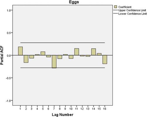
In identifying the model, the ACF is applied in egg consumption data to check if data are stationary. Figure1 shows a very slow linear decay pattern which is a sign of nonstationary time series. This problem can be corrected by a first-degree order of differentiation. After applying autocorrelation, both ACF (Figure 2) and PACF plots (Figure 3) show significant spike only at lag 1 meaning that higher order autocorrelations are explained by the lag 1 autocorrelation. This implies that there is no need of adding AR (p) or MA (q).

Figure 1. Autocorrelation plot of eggs consumption data used to test for stationarity.

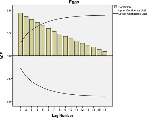
Figure 2. ACF plot after first-order differencing of the eggs consumption data.

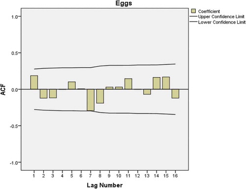
Figure 3. PACF plot after first-order differencing of eggs consumption data.

3.2.2. Parameter estimation and validation

After trial and error, four models are chosen and tested to find a model with low normal BIC. These models include ARIMA(1,1,1), ARIMA(0,1,1), ARIMA(1,1,0) and ARIMA(0,1,0). SPSS is used to estimate each model parameter using ARIMA tab in expert modelers. ACF plots for all the models are within the limit of .2718 (see Figures 4–7), but ARIMA(0,1,0) is observed to have the lowest normal BIC and is chosen as a better model to forecast the consumption of eggs (see Table 1).

Table 1. Results from SPSS after modeling sample models using eggs consumption data

Fit statistic	ARIMA(1,1,0)	ARIMA(0,1,0)	ARIMA(0,1,1)	ARIMA(1,1,1)
Stationary R-squared	.035	6.446E − 016	.046	.049
R-squared	.958	.956	.958	.958
RMSE	1,777.105	1,791.099	1,767.148	1,782.246
MAPE	4.198	4.272	4.219	4.233
MaxAPE	26.995	26.857	26.385	26.046
MAE	1,194.829	1,206.246	1,206.101	1,210.395
MaxAE	7,105.022	7,068.654	6,944.521	6,855.326
Normalized BIC	15.117	15.057	15.106	15.199

Figure 4. Residual plots for ACF and PACF after estimating ARIMA(0,1,0) for eggs consumption.

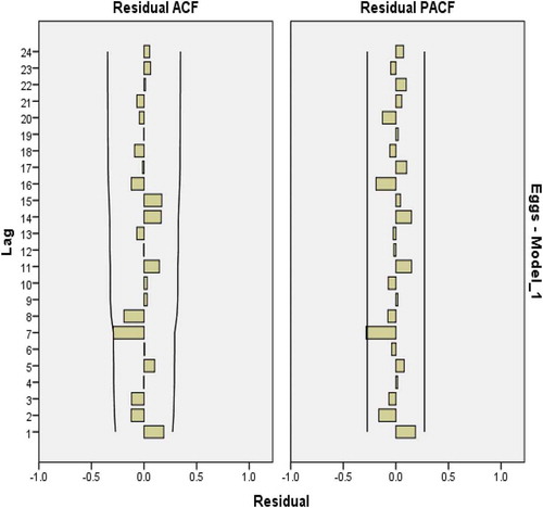
Figure 5. Residual plots for ACF and PACF after estimating ARIMA(1,1,0) for eggs consumption.

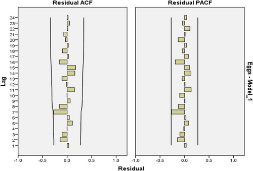
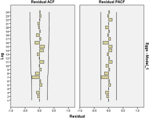
Figure 6. Residual plots for ACF and PACF after estimating ARIMA(0,1,1) for eggs consumption.

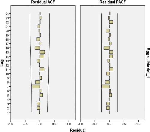
Figure 7. Residual plots for ACF and PACF after estimating ARIMA(1,1,1) for eggs consumption.

ARIMA(0,1,0) model is represented as

${\mathrm{y}}_{\mathrm{t}}={\mathrm{y}}_{\mathrm{t}-1}+{\epsilon }_{\mathrm{t}}$

where y_t is the current production, y_t−1 is the lagged value and ε_t is the error term or the current shock.

From Table 3, the model is presented as

Table 2. Model statistics

SPSS results from ARIMA(0,1,0) using eggs consumption data
Model	Number of predictors	Model fit statistics		Ljung–Box Q(18)			Number of outliers
		Stationary R-squared	Normalized BIC	Statistics	DF	Sig.
Eggs-Model_1	0	6.446E − 016	15.057	19.693	18	.350	0

Table 3. Model parameter

Model parameter results from SPSS for ARIMA(0,1,0) estimated from eggs consumption data
				Estimate	SE	t	Sig.
Eggs-Model_1	Eggs	No transformation	Constant	463.654	248.381	1.867	.068
			Difference	1

${\mathrm{y}}_{\mathrm{t}}={\mathrm{y}}_{\mathrm{t}-1}+463.654+{\epsilon }_{\mathrm{t}}$

Model statistics and parameters for ARIMA(0,1,0) are shown in Tables 2 and 3. The forecast data for egg consumption are presented in Table 4.

Table 4. Forecasted data on consumption of eggs

Forecast
Model		2014	2015	2016	2017	2018	2019	2020
Eggs-Model_1	Forecast	35,493.65	35,957.31	36,420.96	36,884.62	37,348.27	37,811.92	38,275.58
	UCL	39,089.43	41,042.51	42,649.04	44,076.18	45,388.68	46,619.75	47,789.12
	LCL	31,897.87	30,872.11	30,192.89	29,693.05	29,307.86	29,004.10	28,762.04

3.3. Model for consumption of cattle meat

3.3.1. Model identification

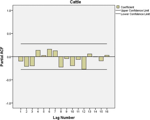
The procedure for building a consumption of meat model is the same as in the eggs model. The ACF is applied in cattle meat consumption data and again a very slow linear decay pattern is observed (see Figure 8). This is a sign of a nonstationarity problem which can be corrected by a first-degree order of differentiation. After applying autocorrelation, both ACF (Figure 9) and PACF plots (Figure 10) show significant spike only at lag 1 as in egg consumption data. This implies that there is no need of adding AR (p) or MA (q).

Figure 8. Autocorrelation plot of cattle meat consumption data used to test for stationarity.

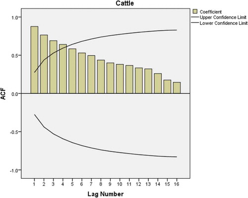
Figure 9. ACF plot after first-order differencing of cattle meat consumption data.

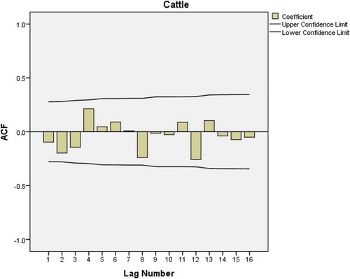
Figure 10. PACF plot after first-order differencing of the cattle meat consumption data.

3.3.2. Parameter estimation and validation

Four models are chosen and tested to find a model with good fit. These models include ARIMA(1,1,1), ARIMA(0,1,1), ARIMA(1,1,0) and ARIMA(0,1,0). The ACF plots of these models are shown in Figures 11–14. All models are within the limit which indicates good fit. Results from SPSS presented in Table 5 are in favor of ARIMA(0,1,0) which has the lowest normal BIC and is chosen as a better model to forecast consumption of cattle meat.

Table 5. Results from SPSS after modeling sample models using cattle meat consumption data

Fit statistic	ARIMA(1,1,1)	ARIMA(0,1,1)	ARIMA(0,1,0)	ARIMA(1,1,0)
Stationary R-squared	.112	.017	−1.02E − 16	.009
R-squared	.914	.905	.903	.904
RMSE	16,910.284	17,606.759	17,584.861	17,676.692
MAPE	5.667	5.721	5.521	5.625
MaxAPE	27.511	31.727	29.405	31.2
MAE	10,363.007	10,421.518	9,989.272	10,200.614
MaxAE	55,471.882	5,7503.44	57,777.288	57,853.404
Normalized BIC	19.699	19.704	19.626	19.712

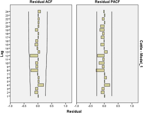
Figure 11. Residual plots for ACF and PACF after estimating ARIMA(0,1,0) for cattle meat consumption.

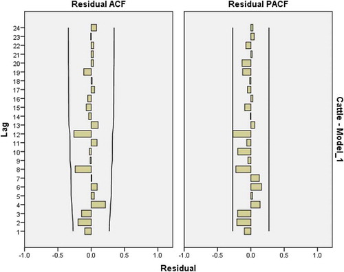
Figure 12. Residual plots for ACF and PACF after estimating ARIMA(1,1,0) for cattle meat for cattle consumption.

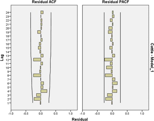
Figure 13. Residual plots for ACF and PACF after estimating ARIMA(0,1,1) for cattle meat consumption.

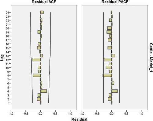
Figure 14. Residual plots for ACF and PACF after estimating ARIMA(1,1,1) for cattle meat consumption.

From Table 7, the model is presented as

${\mathrm{y}}_{\mathrm{t}}={\mathrm{y}}_{\mathrm{t}-1}+4222.712+{\epsilon }_{\mathrm{t}}$

Table 6. Model statistics

SPSS result from ARIMA(0,1,0) using cattle meat consumption
Model	Number of predictors	Model fit statistics		Ljung–Box Q(18)			Number of outliers
		Stationary R-squared	Normalized BIC	Statistics	DF	Sig.
Cattle-Model_1	0	−1.023E − 016	19.626	17.846	18	.466	0

Table 7. Model parameters

Model parameter results from SPSS for ARIMA(0,1,0) estimated from cattle meat consumption data
				Estimate	SE	t	Sig.
Cattle-Model_1	Cattle	No transformation	Constant	4,222.712	2,438.581	1.732	.089
			Difference	1

Model statistics and parameters for ARIMA(0,1,0) are shown in Tables 6 and 7. Forecast data for the cow meat consumption are presented in Table 8.

Table 8. Forecasted data on consumption of cattle meat

Forecast
Model		2014	2015	2016	2017	2018	2019	2020
Cattle-Model_1	Forecast	303,803.71	308,026.42	312,249.13	316,471.85	320,694.56	324,917.27	329,139.98
	UCL	339,106.79	357,952.52	373,395.87	387,078.01	399,634.65	411,391.81	422,543.16
	LCL	268,500.63	258,100.33	251,102.40	245,865.68	241,754.47	238,442.73	235,736.81

3.4. Model for consumption of cow milk

3.4.1. Model identification

To identify the model, the first step is to plot the ACF of the data. The plotted figure shows a very slow linear decay pattern which is a sign of nonstationary time series (Figure 15). This problem can be corrected by a first-degree order of differentiation. Figure 16 shows that autocorrelations are significant for large number of lags. This is because of the propagation of the autocorrelation at lag 1 and can be confirmed in Figure 17 which shows a significant spike only at lag 1 meaning that higher order autocorrelation is explained by the lag 1 autocorrelation. It implies that autocorrelation can be explained more easily by adding AR (p) than MA (q).

Figure 15. Autocorrelation plot of cow milk consumption data used to test for stationarity.

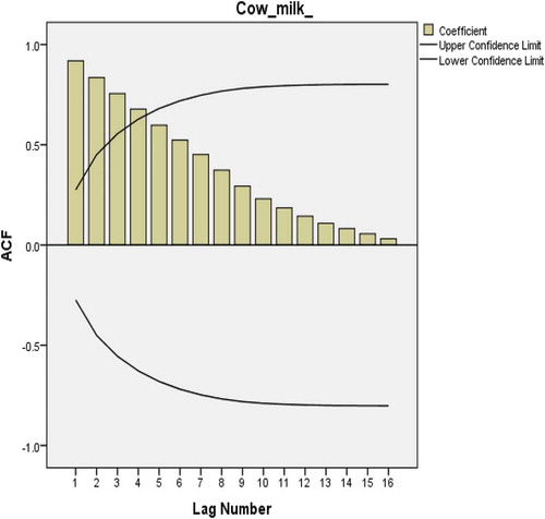
Figure 16. ACF plot after first-order differencing of cow milk consumption data.

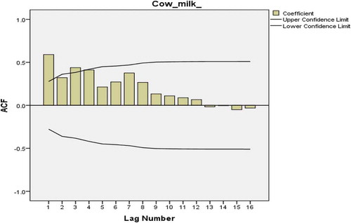
Figure 17. PACF plot after first-order differencing of cow milk consumption data.

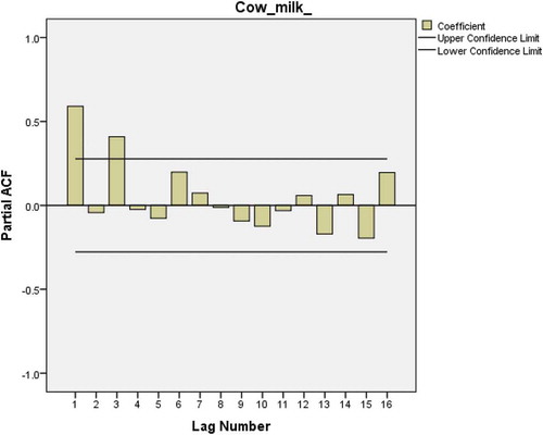
Figure 18. Residual plots for ACF and PACF after estimating ARIMA(1,1,0) for cow milk consumption.

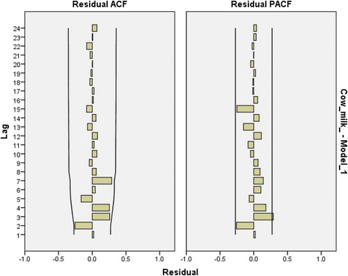
Figure 19. Residual plots for ACF and PACF after estimating ARIMA(3,1,0) for cow milk consumption.

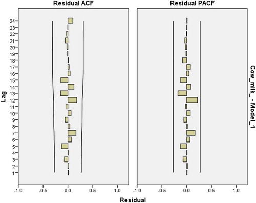
Figure 20. Residual plots for ACF and PACF after estimating ARIMA(3,1,1) for cow milk consumption.

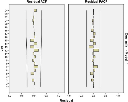
Figure 21. Residual plots for ACFand PACF after estimating ARIMA(2,1,1) for cow milk consumption.

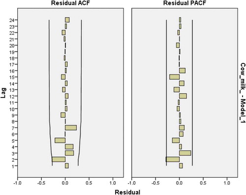
3.4.2. Parameter estimation and validation

Four models are chosen and tested to find a model with a good fit. These models include ARIMA(1,1,0), ARIMA(2,1,0), ARIMA(3,1,0) and ARIMA(3,1,1). The ACF plots in Figures 18–21 show that in the models, the correlation coefficients are within a limit. But the results from SPSS in Table 9 are in favor of ARIMA (3,1,0) which has the lowest normal BIC.

Table 9. Results after modeling sample models from SPSS using cow milk consumption data

Fit statistic	ARIMA(1,1,0)	ARIMA(2,1,0)	ARIMA(3,1,0)	ARIMA(3,1,1)
Stationary R-squared	.353	.354	.426	.472
R-squared	.994	.994	.994	.995
RMSE	38,565.76	38,944.67	36,347.915	35,940.803
MAPE	3.994	4.019	3.566	4.062
MaxAPE	12.527	12.649	10.581	12.537
MAE	25,619.424	25,638.88	23,738.546	24,494.054
MaxAE	138,865.35	139,563.1	120,576.417	121,590.434
Normalized BIC	21.272	21.368	21.154	21.359

ARIMA(3,1,0) is represented as follows:

${{\mathrm{y}}^{\prime }}_{\mathrm{t}}={\mathrm{a}}_1{{\mathrm{y}}^{\prime }}_{\mathrm{t}-1}+{\mathrm{a}}_2{{\mathrm{y}}^{\prime }}_{\mathrm{t}-2}+{\mathrm{a}}_3{{\mathrm{y}}^{\prime }}_{\mathrm{t}-3}+{\epsilon }_{\mathrm{t}}$

where y'_t is the dependent variable; a₁, a₂ and a₃ are the parameters; y'_t−1, y'_t−2 and y'_t−3 are lagged differentiated dependent variables and ε_t is the random error or white noise term (forecast error).

FromTable 11, estimated model is illustrated which can be presented as

${{\mathrm{y}}^{\prime }}_{\mathrm{t}}=0.536{{\mathrm{y}}^{\prime }}_{\mathrm{t}-1}+0{{\mathrm{y}}^{\prime }}_{\mathrm{t}-2}+0.346{{\mathrm{y}}^{\prime }}_{\mathrm{t}-3}+{\epsilon }_{\mathrm{t}}$

Table 10. Model statistics

SPSS result from ARIMA(3,1,0) using cow milk consumption data
Model	Number of predictors	Model fit statistics		Ljung–Box Q(18)			Number of outliers
		Stationary R-squared	Normalized BIC	Statistics	DF	Sig.
Cow_milk_-Model_1	0	.426	21.154	12.120	16	.736	0

Table 11. Model parameters results from SPSS for ARIMA(3,1,0) estimated from cow milk consumption data

ARIMA model parameters
					Estimate	SE	t	Sig.
Cow_milk_-Model_1	Cow_milk_	No transformation	AR	Lag 1	.536	.105	5.093	.000
				Lag 3	.346	.113	3.072	.003
			Difference		1

Model statistics and parameters for this model are shown in Tables 10 and 11. Forecast data for the cow meat consumption are presented in Table 12.

Table 12. Forecasted data on consumption of cow milk

Forecast
Model		2014	2015	2016	2017	2018	2019	2020
Cow_milk_Model 1	Forecast	1,989,163	2,065,002	2,129,413	2.187,344	2,244,678	2,297,735	2,346,253
	UCL	2,062,159	2,198,811	2,318,177	2.441,162	2,569,589	2,694,600	2,817,433
	LCL	1,916,167	1,931,193	1,940,650	1.933,525	1,919,767	1,900,869	1,875,073

3.5. Model for consumption of chicken meat

3.5.1. Model identification

The plot of ACF is created from the data. The plotted figure shows again a sign of nonstationary time series (Figure 22). This problem can be corrected by a first-degree order of differentiation. Figures 23 and 24 show a single spike at lag 1 which is a sign of MA(q) term. Also we can add a second-order differentiation but with no constant (Nau, 2018).

Figure 22. Autocorrelation plot of chicken meat consumption data used to test for stationarity.

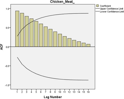
Figure 23. ACF plot after first-order differencing of the chicken meat consumption data.

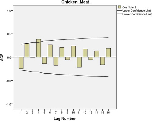
Figure 24. PACF plot after first-order differencing of the chicken meat consumption data.

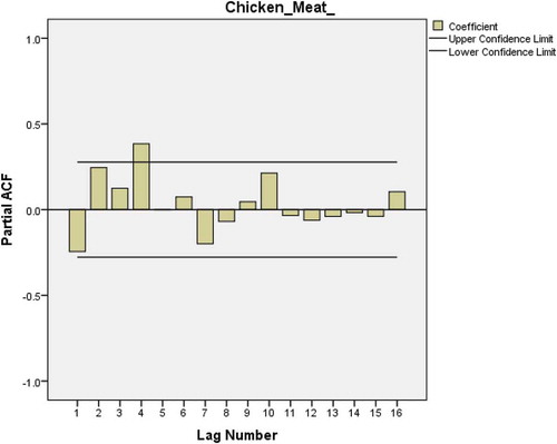
Figure 25. Residual plots for ACF and PACF after estimating ARIMA(0,1,1) for chicken meat consumption.

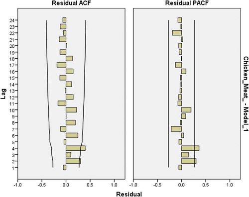
Figure 26. Residual plots for ACF and PACF after estimating ARIMA(0,2,1) for chicken meat consumption.

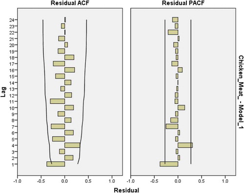
Figure 27. Residual plots for ACF and PACF after estimating ARIMA*(0,2,1) for chicken meat consumption.

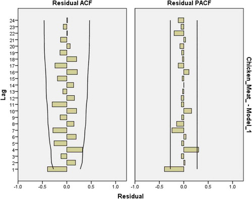
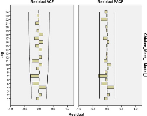
Figure 28. Residual plots for ACF and PACF after estimating BROWN (model) for chicken meatconsumption.

3.5.2. Parameter estimation and validation

Four models are chosen to be tested after trial and error which include ARIMA(0,1,1), ARIMA*(0,2,1),¹ ARIMA(0,2,1) and BROWN models. The Brown model is tested because it is equivalent to ARIMA(0,2,1) and if there is an element of liner trend in the data, smoothing models may be better in forecasting (Alwashali, Fares, & Mohamed, 2015; Nau, 2018). The ACF's of the four models are plotted and the results are shown in Figures 25–28. The results show that all ARIMA models have some coefficients that have passed over the limit of .2718. Only BROWN model has all coefficients within the limit. Again Table 13 shows the results of the four models in which BROWN model is observed to have lower normal BIC.

Table 13. Results from SPSS after modeling sample models using chicken meat consumption data

Fit statistic	ARIMA(0,1,1)	ARIMA*(0,2,1)	ARIMA(0,2,1)	BROWN
Stationary R-squared	.038	.598	.629	.655
R-squared	.986	.986	.987	.988
RMSE	3,065.994	3,121.094	3,031.723	2,838.642
MAPE	8.708	4.833	4.852	5.334
MaxAPE	29.903	18.115	20.356	20.336
MAE	2,000.372	1,794.535	1,739.159	1,764.957
MaxAE	11,184.075	12,595.737	12,470.249	9,983.753
Normalized BIC	16.208	16.169	16.188	15.977

The model is represented as follows:

$\begin{array}{c}\mathrm{i}-1\\ {\hat{y}}_{\mathrm{t}+1}=\alpha \sum {\left(1-\alpha \right)}^{\mathrm{k}}{\mathrm{y}}_{\mathrm{i}-\mathrm{k}}\\ \mathrm{k}=0\end{array}$

where ŷ_t+1 is the forecast value (weighted moving average of all past observation), α is the series weight for each observation and y_i−k are the lagged observations (Ostertagová & Osterta, 2011). After inclusion of the data from Table 15, the model is presented as

Table 14. SPSS result from BROWN model using chicken meat consumption data

Model statistics
Model	Number of predictors	Model fit statistics		Ljung–Box Q(18)			Number of outliers
		Stationary R-squared	Normalized BIC	Statistics	DF	Sig.
Chicken_Meat_-Model_1	0	.655	15.977	25.879	17	.077	0

Table 15. Model parameters

Model parameter results from SPSS for BROWN model estimated from chicken meat consumption
Model			Estimate	SE	t	Sig.
Chicken_Meat_-Model_1	No transformation	Alpha (level and trend)	.401	.059	6.814	.000

$\begin{array}{rl}& i-1\\ & {\hat{y}}_{t+1}=0.401\sum {\left(0.599\right)}^k{y}_{i-k}\\ & k=0\\ & \end{array}$

Model statistics and parameters for this model are shown in Tables 14 and 15. Forecast data for the cow meat consumption are presented in Table 16.

Table 16. Forecasted data on consumption of chicken meat

Forecast
Model		2014	2015	2016	2017	2018	2019	2020
Chicken_Meat_-Model_1	Forecast	90,740.03	92,864.57	94,989.10	97,113.64	99,238.17	101,362.71	103,487.25
	UCL	96,436.18	100,165.75	104,119.85	108,263.18	112,572.68	117,032.35	121,630.42
	LCL	85,043.88	85,563.38	85,858.36	85,964.10	85,903.67	85,693.07	85,344.08

Overall results from all four estimated models show that production of all livestock products will increase (Table 17). Cow milk is going to be consumed most in the future, followed by chicken and cattle meat. This is expected to increase demand for animal feed and is an opportunity for sorghum and millet farmers to capture new markets in animal feed if they can produce enough to keep up with the increase in demand.

Table 17. ARIMA Model, forecasts and annual rates of growth for livestock products from 2016 to 2020, Tanzania

Livestock product	Model Type	Production forecast in tons
		2016	2017	2018	2019	2020	%*
Eggs	ARIMA(0,1,0)	36421	36885	37348	37812	38276	1.0186
Chicken	BROWN	94989	97114	99238	101363	103487	1.7893
Milk	ARIMA(3,1,0)	2129413	2187344	2244678	2297735	2346253	2.0366
Cattle	ARIMA(0,1,0)	312249	316472	320695	324917	329140	1.0819

%*- Average annual growth rate from 2016-2020

4. Conclusion

The animal feed industry is one of the potential opportunities for sorghum and millet market. As population and income grow, the demand for livestock products (such as meat, milk and eggs) is expected to grow. As a consequence, the demand for animal feed is expected to increase also.

At the moment, efforts should be done to encourage the use of sorghum and millet in animal feed which will help to reduce humans and livestock competition over maize. As long as there is market for sorghum and millet in feed industries, smallholder farmers in semiarid region will be encouraged to abandon traditional crops which are rain dependent. This will improve their livelihood and reduce poverty in these areas.

Forecast done in this study does not consider some other factors that may influence consumption of livestock product. For instance, in recent years, population growth rate has been very high which will also have positive effect on the consumption of livestock. Another factor which may have an impact is a change of eating behavior. In recent years, people have learnt much about eating healthy which may have effect on the consumption of livestock products which are argued to be unhealthy, especially red meat. Hence, more research works are needed to understand by how much both of these two factors may affect the consumption of livestock products so as to measure real opportunity for sorghum and millet farmers to capture market in feed industry.

Cover image

Source: Author.

Additional information

Funding

The author received no direct funding for this research.

Notes on contributors

Joseph Frank Mgaya

Joseph Frank Mgaya is an assistant lecturer at the department of Accounting and Finance in the University of Dodoma. For the past nine years, he has been teaching different courses in the department related to accounting and finance. His research interest is mainly in rural development, especially in rural finance, agricultural improvement and agribusiness. Recently, he has gain interest in different econometric models such as forecasting models which are crucial in policy planning and development.

This paper has reported an opportunity in the feed industry which can be utilized by farmers in semiarid regions to involve themselves in drought resistance crops such as sorghum and millet. As maize is preferred than sorghum and millet, linking farmers in feed industry is important. Substituting maize with sorghum and millet will be advantageous to the society as it will eliminate competition between animals and humans in the consumption of maize.

Notes

1. ARIMA*(p,d,q) is an ARIMA model which does not include a constant term.

References

- Abdulkadir, D. I., Na-Allah, Y., & Bala, A. G. (2013). A review - The use of sorghum as a substitute to maize in poultry feed production. Drylands, Katsina State Agricultural and Rural Development Authority, Katsina, Nigeria.
- Alwashali, E., Fares, M., & Mohamed, F. (2015). Prediction of cholera incidence by using the comparison of four models: Autoregressive integrated moving average model, Holt model, Brown model and simple regression model. International Journal of Tropical Disease & Health, 9, 1–29. doi:10.9734/IJTDH/2015/18115
- Amani, H. (2005). Making agriculture impact on poverty in Tanzania: The case on non traditional export crops. Policy dialogue for accelerating growth and poverty reduction in Tanzania. Dar es Salaam: Economic and Social Research Fund.
- Blum, A., & Sullivan, C. Y. (1986). The comparative drought resistance of landraces of and sorghum millet from dry and humid regions. Annals of Botany, 57, 835–846. doi:10.1093/oxfordjournals.aob.a087168
- Box, G. E. P., Jenkins, G. M., & Reinsel, G. C. (1994). Time series analysis; Forecasting and control. 3rd edition, Prentice Hall, Englewood Cliff, New Jersey.
- Chauvin, N. D., Mulangu, F., & Porto, G. (2012). Food production and consumption trends in Sub-Saharan Africa: Prospects for the transformation of the agricultural sector, African center for economic transformation. New York, NY: UNDP Regional Bureau for Africa.
- FAOSTAT. (2014). Livestock consumption data. Rome: Food and Agriculture Organization of the United Nations.
- Group, C.-D. S. (2011). Effective support for agricultural development in Tanzania. China: International Poverty Reduction Center.
- Issa, S., Jarial, S., Brah, N., Harouna, L., & Soumana, I. (2015). Use of sorghum on stepwise substitution of maize in broiler feeds in Niger. Inran/Icrisat, 27(10), 1–6.
- Jose, J., & Sojan, P. (2013). Application of ARIMA(1,1,0) model for predicting time delay of search engine crawlers. Informatica Economică. Bucharest, Department of Computer Applications, BPC College Piravom, Kerala, India. doi:10.12948/issn14531305/17.4.2013.03
- Majid, K. D. (2008). Tanzania’s creative solutions in response to global food crisis. Tanzania: Sokoine University of Agriculture.
- Mandal, B. N. (2005). Forecasting sugarcane productions in India with ARIMA model. New Delhi: IASRI.
- Nau, R. (2018). ARIMA models for time series forecasting. Retrieved from https://people.duke.edu/~rnau/411arim.htm
- Neath, A., & Cavanaugh, J. (2012). The Bayesian information criterion: Background, derivation, and applications. Wiley Interdisciplinary Reviews: Computational Statistics, 4(2), 199–203. doi:10.1002/wics.199
- Ostertagová, E., & Osterta, O. (2011). The simple exponential smoothing model. The 4th International Conference of Mechanical Engineering, Technical University of Kosice, Slovakia.
- Ramasubramanian, V. (2001). Time Series Analysis. New Delhi: I.S.R.I.
- Raymond, Y. C. (1997). An application of the ARIMA model to real-estate prices in Hong Kong. Journal of Property Finance, 8(2), 152–163.
- Rohrbach, D., & Kiriwaggulu, J. A. (2001). Commercialization prospects for sorghum and pearl millet in Tanzania. Working Paper Series no, 7, Bulawayo Zimbabwe/Socioeconomic and Policy Programme, ICRISAT.
- Studenmund, A. H. (2016). Using econometrics: A practical guide (4th ed.). Pearson, USA. ISBN 10: 013418274-X.
- Government of Tanzania (2014). 2012 population and housing census. National Bureau of Statistics & Office of Chief government statician, Tanzania.
- Yeboah, S. A., Ohene, M., & Wereko, T. B. (2012). Forecasting aggregate and disaggregate energy consumption using Arima models: A literature survey. Journal of Statistical and Econometric Methods, 1(2), 71–79. ISSN: 2241 (print), 2241-0376 (online) Scienpress Ltd., 2012.