Determinants of household dietary diversity in the Yayo biosphere reserve of Ethiopia: An empirical analysis using sustainable livelihood framework

Abstract

Household dietary diversity (HDD) is an important nutrition outcome measuring the economic ability of a household to access a variety of foods during a determined period. For this, it has been increasingly used as indicator of food security. This paper examines the determinants of HDD. Data for this paper comes from the cross-sectional survey collected from two districts of Illu Ababora Zone, Oromia region of Ethiopia. Overall, 334 farm households of which 71 female headed households and 263 male headed households were surveyed. Twelve different food groups were used to calculate the HDD score, which is a continuous score ranging from 0 to 12. This score was then recoded to a three-level ordered categorical variable. Ordered probit, OLS regression and Poisson regression were used to check for robustness and consistency of the results. The result shows that human capital, natural capitals and physical capitals are the main explanatory factors for HDD variations in the study context. Mediating the utilization of livelihood assets, social relations, institutions, organizations, shocks and seasonality are also explaining variations in HDD. Livelihood strategies such as farm production diversity and non-farm income are significantly and positively influencing HDD. Similarly, livelihood outcomes such as meal frequency and household wealth status are also positively influencing HDD. The current promotion of export crops at the expense of crops diversity will hurt HDD given the apparent poor market-integration, rugged terrain, poor infrastructure development and fragmented institutional arrangements at the study areas.

Keywords:

• farm diversity
• biosphere reserve
• dietary diversity
• livelihood
• ordered probit

Public interest statement

Household dietary diversity (HDD) is an important nutrition outcome measuring the economic ability of a household to access a variety of foods. Monotonous low quality diets are becoming the norm in resource-limited environments of most rural areas of Ethiopia. Evidences shows that farm households with small farm size are less likely to diversify their farm production and hence less potential to diversify their dietary. On the other hand, the current agricultural policy of Ethiopia gives more emphasis to the promotion of export crops at the expense of crop diversity. Thus, there is heightened need for empirical assessment of the determinants of household dietary diversity with the objective to inform the policy-makers. Publication of this work will advance knowledge of the determinants of farm and dietary diversity in the context where farmers are facing farm size shortage coupled with other institutional and cultural constraints acting as a brake on nutrition security

Competing Interests

The authors declares no competing interests.

1. Introduction

Food security and its implication for health have long been and is still one of the global concerns. Given the strong link between the two, proper measurement of food security affects the development of policies on the improvement of the later (Cordero-Ahiman, Santellano-Estrada, & Garrido, 2017; Fanzo et al., 2013). As food security is an abstract term, its measurement depends on how we define and conceptualize it. According to the World Food Summit 1996, “food security exists when all people, at all times, have physical and economic access to sufficient, safe and nutritious food that meets their dietary needs and food preferences for an active and healthy life“ (WFP, 2009).

Strongly linked to this definition, four main dimensions of food security are identified. This includes food availability, food access, food utilization and stability (FAO, 2008; Hoddinott & Yohannes, 2002; WFP, 2009). While food availability is related to the physical presence of food in the area through all forms of domestic production, commercial imports and food aid, food access is concerned with the household’s ability to acquire adequate amounts of food, through one or a combination of own home production and stocks, purchases, barter, gifts, borrowing and food aid (Jemal & Kim, 2014; Nkegbe, Abu, & Issahaku, 2017; WFP, 2009). Thus, food may be available but not accessible to certain households during a given period of time if they cannot acquire a sufficient quantity or diversity of food through these mechanisms (Fanzo, 2017; Fanzo et al., 2013; WFP, 2009). This necessitates the development of methodological tools to identify and assess the different dimensions of food security.

Household Dietary Diversity Score (HDDS) is a qualitative methodology that has been validated in different countries as an approximate measure of food availability and food accessibility aspects of food security (Cordero-Ahiman et al., 2017; Hoddinott & Yohannes, 2002; Ruel, 2003; WFP, 2009). HDDS assesses the number of different food groups consumed in the household during a defined reference period, such as the last 24 or 48 hours or the last 7 or 14 days (Cordero-Ahiman et al., 2017; FAO, 2008; Koppmair, Kassie, & Qaim, 2016; WFP, 2009). Thus, a diversified diet is linked to the economic ability of a household to access a variety of foods by obtaining a number of different food groups consumed during a determined period. In other words, increase in dietary diversity is associated with socio-economic status and household food security.

Hunger and malnutrition remain among the most devastating health problems in Ethiopia. According to the Ethiopia Mini Demographic and Health Survey (EMDHS, 2019), 36.8% of children under the age of five are found to be stunted, 21.1% are underweight, and 7.2% are wasted. These rates are fairly above the rates considered as sever health problem. WHO (2006) defines stunting and underweight prevalence rate of over 30% and 20% respectively as high and a major public health problem. Thus, food insecurity and the related health problems remains the Ethiopia’s priority agenda.

Food insecurity and malnutrition problems are even higher in rural populations plagued with small farm size hindering production diversification; weak institutional arrangements, and weak market integration (EMDHS, 2019; Abay & Melese, 2019; Abduselam, 2017; Hirvonen & Hoddinott, 2014; Jemal & Kim, 2014; Koppmair et al., 2016; Sisay, Mulugeta, & Molla, 2019; Wondimagegnhu, Admassu, & Nischalke, 2019). The situation could be more worse for those rural households of Yayo and Hurumu districts of Oromia region, who are living in the areas of protected biosphere reserves (Wondimagegnhu et al., 2019). As there has been legal restriction prohibiting free movement in the protected areas either for farm expansion or for hunting, food availability and food access situation of those rural households could be further curtailed thereby resulting in the lower dietary diversity score.

Thus, examining the determinants of household dietary in the context of the biosphere where farm land scarcity is prominent (Wondimagegnhu et al., 2019) makes it particularly relevant given the widespread prevalence of food insecurity and malnutrition, cash crops promoting kind of agricultural policy currently promoted despite the poor household nutritional status, as well as the fact that more 95% of the population depends on agriculture as a source of livelihood (Wondimagegnhu et al., 2019). Accordingly, this paper addresses a research question: What are the main determinants of household dietary diversity (HDD) in the Yayo biosphere reserve of Oromia region? As analytical too, we used Sustainable Livelihood Framework (SLF). According to SLF (Jemal & Kim, 2014), HDD is the function of its asset endowments: human capital, social capital, financial capital and natural capital mediated by such factors as social relations, institutions and organizations bounded with trends, shocks and seasonality. To the best of our knowledge, the current paper is unique in applying SLF and hence provides more comprehensive analysis of the determinants of HDD.

The rest of the paper proceeds as follows. Section 2 explains study site, descriptions of the nature of data, measurement of variables and analytical methods are explained. Section 3 presents results and discussion. Descriptive statistics is first provided followed by results of rigorous econometric results with detailed discussion. The last section summarizes the paper.

2. Literature review

2.1. Definitions and measurements of food security

The concept of food security is complex and hence its definition has been evolving over time. According to the United Nations in 1974, food security was defined as “availability at all times of adequate world food supplies of basic foodstuffs to sustain a steady expansion of food consumption and to offset fluctuations in production and prices”. This definition measures the ability of a nation to assure sufficient quantity of food supply for its current and future generations but fails to measure the quality of food (Nkegbe et al., 2017). Recognizing this limitation, the World Bank has revised the definition of food security as “access by all people at all times to enough food for an active and healthy life” (World Bank, 1986). Implicit within this definition, the quality of food has came to an agenda. However, the most comprehensive definition of food security was adopted during the 1996 World Food Summit which read as “Food security exists when all people, at all times, have physical and economic access to sufficient, safe and nutritious food that meets their dietary needs and food preferences for an active and healthy life” (WFP, 2009).

This latest definition is widely accepted because it “accommodates and reflects the complex arguments of nutrition and human rights in food security” (Nkegbe et al., 2017). Furthermore, it adequately addresses such issues as inequitable distributions of food not only within a country but also within households, the ability to acquire socially and culturally acceptable food, the way it is acquired, as well as macro and micro-nutrient compositions of the food (Daniel & Gerber, 2017).

According to this latest definition, food security consists of four essential parts: food availability, food access, food utilization and stability (IFPRI, 2017; Jemal & Kim, 2014; Muro & Mazziotta, 2011; Nkegbe et al., 2017). The first component measures the availability of food in a given country or household through any means such as production, imports or food aids. The second component measures the “physical, economic and social access” to food by all people or households as reflected by their ability to get food through purchase from market or from own stock (Jemal & Kim, 2014; Muro & Mazziotta, 2011; Nkegbe et al., 2017). The third component is concerned with the actual food processing and absorption capacity of the supplied nutrient by the body while stability measures presence of food at all times in terms of availability, access and utilization for food security to exist (Harris-Fry et al., 2015).

The first three components are physical determinants while the fourth component is the temporal determinant. Both the physical determinants and temporal determinant are strongly interlinked and hence shortfall in any of the components will ultimately affect the others (Jemal & Kim, 2014). For example, food might be available but may not necessarily food is accessible to all people; similarly, access might be viable but does not guarantee utilization and all three can be disrupted by a lack of stability caused by climate change, conflict, unemployment, disease or other factors (Muro & Mazziotta, 2011). Likewise, stability or the lack of it can affect any or all of the other three components of the food insecurity components.

2.2. Dietary diversity as a measure of food security

Dietary Diversity scores are defined as the number of foods or food groups consumed by an individual (IDDS) or by any member of the household inside the home (HDDS) over a reference time period (FAO, 2008). Thus, dietary diversity data can be collected either at household level or individual level. While HDDS measures the economic ability of the household to access a variety of foods, Individual Dietary Diversity Score (IDDS) is often used as a proxy measure of the nutritional quality of an individual’s diet (WFP 2009, FAO, 2008; Harris-Fry et al., 2015).

Evidences show that HDDS is widely recognized as an appropriate measure of food security proxying food access and availability aspects (WFP 2005; Harris-Fry et al., 2015; Jones, 2017). Examining the determinants of HDD is important to know what determines the availability as well as access to food (Jemal & Kim, 2014). While factors that affect food availability operate on the demand side, determinants of access to food operate on the supply side. Thus, factors that affect the demand for and supply of food affects availability and access to food and eventually affects household food security (Babatunde, Omotosho, & Sholotan, 2007; Jemal & Kim, 2014; Jones, Shrinivas, & Bezner-Kerr, 2014).

2.3. Determinants of household dietary diversity

A number of socio-economic factors were identified as the determinants of HDD studies. In their study to identify the determinants of household dietary practices in rural Tanzania, the authors have pointed out that the literacy status of the mothers, prior nutrition training/knowledge, cultivated land size, and distance to a water source statistically and significantly influence HDD (Mbwana, Kinabo, Lambert, & Biesalski, 2016). Using in-depth qualitative ethnographic research approach (Powell, Kerr, Young, & Johns, 2017) have also identified a number of factors influencing HDD in Tanzania. Among these, spatial and temporal availability of diverse foods, wealth status of the households, diversity of agricultural production and agro biodiversity, household size, personality and tradition, and gender of the household head were found to have significantly influenced HDD.

Control of income within households may have a strong influence on household diets and health outcomes (Jones et al., 2014). Similarly, other evidences showed that ownership of land, reduced risk of food insecurity, wealth status of the household, empowering women over control of economic resources, access to media and literacy statistically and significantly influence HDD (Harris-Fry et al., 2015; Mbwana et al., 2016).

According to Jones et al. (2014), farm production diversity is associated with greater HDD in Malawi. Similarly, other studies also confirm that farm production diversity strongly influences the HDDS (Cordero-Ahiman et al., 2017; Fanzo, 2017; Hirvonen & Hoddinott, 2014; Koppmair et al., 2016; Nkegbe et al., 2017). According to these sources, two production diversity indicators can be calculated. These are (1) count of the number of crop species produced on a farm; and (2) production diversity score defined as the number of food groups produced. To better account for the dietary perspective, it is recommended to use a production diversity score rather than just simple species count of the number of crop species produced on a farm (Hirvonen & Hoddinott, 2014; Koppmair et al., 2016; Nkegbe et al., 2017; Sibhatu, Krishna, & Qaim, 2015). Evidences also showed that inclusion of livestock into farm diversity measures would lead to different results than when it is excluded from the index. According to a study by Jones et al. (2014) in the rural community of Malawi, negative association was observed between the diversity of farms and diets when excluding livestock from the farm diversity measure and the result turned out to be significantly and positively associated with the inclusion of livestock. Thus, it can be safely concluded that lack of production diversity is the major factor restricting access to varied and notorious food and thereby poses public health challenges.

According to the World Health Organization, as many as 30 biologically distinct variants of foods should be consumed each week for dietary diversity required for a healthy life (WHO/FAO, 2006). This is because adequate human nutrition involves regular intake of a wide range of nutrients. Studies also show that a varied, nutritional and balanced diet reduces the malnutrition rates by preventing lack or excess of nutrients in the diet (Cordero-Ahiman et al., 2017; Jones et al., 2014).

Recent studies reveal that food-related expenditures may directly influence the quantity and quality of household diets, while non-food expenditures, through substitution effects, may indirectly influence the amount of resources available for diversifying diets (Jones et al., 2014; Powell et al., 2017). Households with higher food consumption expenditure are less likely to experience low dietary diversity and more likely to experience higher dietary diversity score (Babatunde et al., 2007).

3. Methods

3.1. The study sites

Yayo biosphere reserve is situated in South Western Oromia region. It encompasses six districts: Hurumu, Yayo, Chora, Nopha, AlgeSachi and Doreni Woredas, in Illu Abba Bora Zone (Wondimagegnhu et al., 2019). The biosphere plays a key role in the conservation of natural and cultural landscapes. It is one of the last remaining rainforest fragments with organic Coffee Arabica populations in the world and also an important hotspot for biodiversity and bird species. For these and other cultural reasons, United Nations Educational, Scientific and Cultural Organization (UNESCO) registered the biosphere reserve in 2010 and recognized its international importance. Biosphere’s recognition by the international organization, UNESCO, is an opportunity for sustainable management and development of the reserve (Wondimagegnhu et al., 2019).

For those households living within the vicinity of the biosphere reserves, however, the registration of this reserve by UNESCO could entail both opportunities and threats (Wondimagegnhu et al., 2019). The opportunity is that the reserve will be sustainably managed and developed while the threats are more diverse in nature. Firstly, those households can no more encroach into the protected areas for additional farm land. The household small farm land size is getting smaller and smaller because of the growing population necessitating reallocation of land to their children. This is because as household sizes change over time and new households appear, there is also a need to redistribute land at later stages. At the moment, the average land for cropping (excluding coffee land) is 0.36 ha compared to the national average of 1.63 ha of cultivated land holding per household (Sibhatu et al., 2015). Secondly, the farmers are losing most of their limited crops on the limited land size because of wild life damages. Following the legal protection banning hunting of the wild lives within the vicinity of the reserve, wildlife population is rapidly growing thereby threatening the production of major food crops. Thirdly, because of the legal restrictions to encroach into the protected areas, the farmers can hardly supplement their food by hunting.

Specialization in coffee crop production is the other important peculiarity of the farmers in the study areas. In Yayo and Hurumu districts where coffee grows well, the development agents (DAs) usually advise the farmers to specialize with coffee production. The notion is that diversification might prevent gains from specialization on the farm and could thus result in income losses. However, while this approach is justified on the basis of economic principles, its effect on HDD could be adverse because of lack of crop diversification coupled with weak institutional arrangement and weak market integration (Abay & Melese, 2019; Jones et al., 2014; Koppmair et al., 2016). Although specializing in coffee production could have helped in boosting national coffee export earning, displacing vegetables and fruits with such cash crops production may have contributed to declines in the nutritional quality of household diets. Such cash crops–driven agricultural systems tend to emphasize production of few crops while de-emphasizing production of diverse macro- and micronutrients for human consumption (Fanzo, 2017; Fanzo et al., 2013).

3.2. Study design and data collection procedures

Data for this paper comes from the cross-sectional survey collected in March and April 2016 in Yayu and Hurumu, two districts of Illu Ababora Zone, Oromia region of Ethiopia. The survey was conducted to obtain pre-intervention (baseline) information in districts before the implementation of NutriHAF Africa project.¹ During our survey details on household demographics, household socio-economic status, agricultural production and marketing and consumption of food and non-food products was captured. A special section with a 24 hour food consumption recall captured dietary patterns of the household. In this case, only the women who are customarily involved in the preparation of food were interviewed both in male-headed and female-headed households.

For this household survey, we have collected gender disaggregated data from four villages of Yayuand Hurumu districts. Adopting Yamane² (1967) formula for minimum sample size determination, 334 smallholder farmers were selected using stratified sampling techniques. The sample was stratified in terms of male and female-headed households for comparison purposes. Further stratification was also done with respect to the study villages to ensure their representation in the total sample. Out of 334 farm households, 71 (21%) were female-headed households while the remaining 263 (79%) were male-headed households. However, excluding those cases that had missing data for relevant variables, we restricted our analysis to 306 observations. As all adult members of the same household customarily eat from the same plate in the study areas, sex disaggregated analysis is hardly possible from this data set. However, disaggregated data analysis was made based on the sex of the household head: male-headed household versus female-headed households.

The survey team was led by two postdoctoral researchers with careful selection and intensive training of experienced local enumerators who are conversant with the local community. Sensitive sections, such as the 24 hour consumption recall, were especially emphasized during the training and the pre-testing of the questionnaire. Enumerators were carefully trained to not only focus on the main meals consumed in the household, but to also obtain details on snacks and all ingredients of mixed dishes. Though unique sets of survey questionnaires were developed for both male headed and female headed household, in both cases, mothers were asked a series of questions about contents of food they prepared for their respective households during the past 24 hours. Finally, FAO (2010) guidelines were used for calculating HDDS.

3.3. Measurements

3.3.1. Measurement of dietary diversity

Following FAO (2010), food items were categorized into 12 different food groups with each food group counting toward the household score if a food item from the group was consumed by anyone in the household in the previous 24 hours. The food groups used to calculate this HDDS included: cereals; white tubers and roots; legumes, nuts, and seeds; vegetables; fruits; meat; eggs; fish and fish products; milk and milk products; sweets and sugars; oils and fats; and spices, condiments, and beverages. Thus, the HDDS is a continuous score that can range from 0 to 12 based on whether the household consumed each of the following 12 food groups (FAO, 2007). This score was then recoded to a three-level categorical variable using some cut-off values indicating low dietary diversity, medium dietary diversity and HDD categories. However, as there is no international consensus on which cut-off values to use (Cordero-Ahiman et al., 2017), we have used HDDS less than or equal to three as low dietary diversity group and between four to six as medium category while HDDS greater than or equal to seven as high diversity score category. That is 1 stands for low HDDS of ≤3 (N = 58); 2 stands for medium HDDS of 4–6 (N = 186); and 3 for high HDDS of 7–12 (N = 64). We have considered HDDS ≤ 3 as low dietary diversity score because as a general rule, consumption of four food groups over 24 hours is considered as good dietary diversity (FAO, 2008).

3.3.2. Measurement of other independent variables

Following the suggestion of Jones et al. (2014), we have included agricultural production diversity indicator, including livestock into the HDDS measure. For this, farmers were asked to report details of their farm production and livestock they kept for the last 12 months. Based on this agricultural data, two production diversity indicators were calculated. These are (1) count of the number of crop species produced on a farm; and (2) production diversity score defined as the number of food groups produced. To better account for the dietary perspective, it is recommended to use a production diversity score rather than just simple species count of the number of crop species produced on a farm (Hirvonen & Hoddinott, 2014; Koppmair et al., 2016; Nkegbe et al., 2017; Sibhatu et al., 2015). Thus, we report our result using mainly production diversity score. To construct the production diversity score, we considered the same 12 food groups that we used to construct HDDS. Hence, if a farmer produces several species that belong to the same food groups, the production diversity score will be smaller than the simple species count. For comparison, however, we also report results of econometric models estimated with a simple crop species count as the indicator of farm production diversity (for details, please see section in annex “f”).

To account for intra-household control of resource allocation decisions, we included number of household members with the highest level of educational achievement by female and male members. Control of income within households may have a strong influence on household diets and health outcomes (Jones et al., 2014). Respondents were asked to report whether any household member has received formal education and if so whether the one with better education is female or male member. Here, it is postulated that households with the highest degree of educational achievement by female member will lead to equitable distribution of intra-household resources and hence better dietary diversity.

Following recent literatures, we have included logarithms of household food expenditures per capita as well as logarithms of non-food expenditures per capita of each household. We have also included farm land under control of each farmer measured in terms of farm size in hectare. Dummies for household wealth ranking were also included. As the rural households in the study areas were priory classified into three wealth ranks by the local government,³ the enumerators were simply asking each household head within which wealth group he/she was classified. Finally, a categorical variable named “status” was created where 1 stands for poor household, 2 for middle level and 3 representing rich households. From this categorical data, three dummy variables were created each for the wealth ranks. We also included in our models the number other variables: age of household heads in years; wealth status of each households; whether the household is literate or not; farming experiences of the household heads; average working hours of household heads per day; number of household members with farm experiences; access to credit; access to irrigation; meal frequency of each household over 24 hours; home gardening; distance from near markets in minutes as well as location of each households. In sum, we have considered important variables based on recent literatures.

3.4. Conceptual framework

The conceptual framework for this paper is based on the understanding that food and nutrition insecurity and malnutrition are strongly related to the household livelihoods. Accordingly, Sustainable Livelihood Framework (SLF) is used to identify the explanatory variables.

This framework places emphasis on an “all-round” view of the livelihood circumstances of the households, including their asset status, the activities in which they engage, the chief sources of vulnerability they confront and the encouraging or discouraging character of the institutional context within which their livelihood strategies operate (Ashley, 2000; Carney, 1999; Ellis, 1999; Scoones, 1998). According to this framework, HDD is the function of different household livelihood assets: human capital, natural capital, physical capital, financial capital and social capital. And access to these capitals is modified by social relations, institutions and organizations and mainly influenced by trends, shocks and seasonality resulting in different livelihood strategy choices, which, in turn, results in different livelihood outcomes, including variations in the dietary diversity (please refer to Annex g for details).

3.5. Analytical methodology

3.5.1. Models

As explained above, the HDDS is converted into categorical and ordinal measures. For such ordered discrete variables, ordered probit or logit models are the most appropriate for analysis (Maddala, 1983) for multinomial logit or probit models would fail to account for the ordinal nature of the dependent variable (Greene, 2003; Maddala, 1983). While the logit assumes a logistic distribution of the error term, the probit assumes a normal distribution. Of course, the logistic and normal distributions generally give similar results in practice. However, ordered probit is the most widely used model for ordered response (Nkegbe et al., 2017). Therefore, the ordered probit model is used in this study.

Accordingly, we have specified the probit model as follows. Assume unobservable random variable y_i* as dependent while treating y_i the observed variable, as a categorical variable with “j” response categories and also as a proxy for the unobserved latent random y_i*. Following Nkegbe et al. (2017), the probit model is specified as:

(1) $y_i^{\ast }=x{ }_i^{\prime }\beta +{\epsilon }_i,i=1,2,\mathrm{3....}N$(1)

y_i* is the hypothesized predicators of HDD, βs is a vector of parameters to be estimated and ${\epsilon }_i$is an error term which is assumed to be normally distributed. Then, the values for the observed variable y_i are assumed to be related to the latent variable y_i* in the following manner:

(2) $y=j,if{\mu }_j-1<{y^{\ast }}_i\le {\mu }_j,j=1,2,3,,,,j$(2)

Where µ refers to the unknown threshold parameters, $u-1=-\mathrm{\infty },u0=0,uj=\mathrm{\infty }$ and the estimated cut-off points, µ follows the order${\mu -1}_{\hspace{0.17em}}<{\mu }_0<{\mu }_1{.............<{\mu }_j}_{\hspace{0.17em}}$. The probabilities that a given household will fall within a response category of j follows:

(3) $\begin{array}{rl}& p_{ij}=p\left(y_i=j\right)=p\left(u_j-1<y_i^{\ast }\le u_j\right)=F\left(u_j-x_i^{\prime }\beta \right)-F\left(u_{j-1}-x_i^{\prime }\beta \right)\end{array}$(3)

where F′ (·) is the standard normal cumulative distribution function and j is the response categories, in this case 1, 2 and 3 since there are three categories for HDD.

Marginal effects measure the effects of changes in the explanatory variables on cell probabilities. The ordered probit model with j alternatives will have j sets of marginal effects. Accordingly, the marginal effect of an increase in a regressor x on the probability of a household falling within j response category is given by:

(4) $\begin{array}{rl}& \frac{{\mathrm{\partial }p}_{ij}}{{\mathrm{\partial }x}_{ri}}=\left\{F^{\prime }\left(u_{j-1}-x_i^{\prime }\beta \right)-F^{\prime }\left(u_j-x_i^{\prime }\beta \right)\right\}=\left\{F^{\prime }\left(u_{j-1}-x_i^{\prime }\right)-F^{\prime }\left(u_j-x_i^{\prime }\right)\right\}\beta \end{array}$(4)

Where F′ (·) being the standard normal density function. Then, following (Nkegbe et al., 2017) the final estimated model is specified as:

(5) ${DD}_{ij}=\alpha +\beta W_i+{\gamma X}_i+{\delta Y}_i+{\lambda Z}_i+{\epsilon }_i$(5)

where DD is HDD; subscript i represents a household, subscript j (j = 1, 2, 3) represents the dietary diversity categorization of alternative dependent dummy variables indicating (i) whether a household falls within low dietary diversity category, (ii) whether a household falls within medium dietary diversity category, and (iii) whether a household is within higher dietary diversity category; W, X, y and Z are, respectively, household livelihood assets, mediating factors influencing the use of those assets, livelihood strategies and livelihood outcomes; $\alpha$, $\beta$, $\gamma$, $\delta$, $\lambda$ are parameters to be estimated and $\epsilon$ $\approx$NID(0, 1). Finally, maximum likelihood technique was used to estimate the values for the parameters (please refer to Table 1 below for the detail descriptions and measurement of the explanatory variables).

Table 1. Description, measurement and statistics of explanatory variables

Descriptions and measurements	Obs	Mean^4	Std. Dev.
Household Dietary Diversity Score	306^5	5.23	1.89
Human capital
Education of household head (1 = read & write)	334	70%
Household size (N0)	334	4.71	1.94
N0 of household members with highest degree (M)	334	0.34	0.82
N0 of household members with highest degree (F)	334	0.26	0.67
Whether household head received vocational training (1 = yes)	334	57%
Members with farm experience (N0)	334	1.98	1.86
Household head farming experience (years)	334	22.94	12.77
Financial capital
Access to credit (1 = yes)	334	40%
Physical capital
Residence district (1 = Hurumu)	334	58%
Distance from market (minutes)	334	95.56	74.74
Natural capital
Household Land size (ha)	334	1.28	1.97
Size of home gardens (ha)	334	0.14	1.10
Household access to irrigation (1 = yes)	334	15%
Mediating factors:
Sex of the household head (1 = male)	334	79%
Age of the household head (years)	334	42.34	13.46
Household head working hours during peak times/day	334	6.992	1.83
Primary cooperative membership (1 = yes)	334	80%
Household worry about crops damage by wildlife (1 = yes)	333	43%
Livelihood strategies
Production diversity score (variety groups)	334	2.58	1.18
Crop species grown (species count)	334	3.77	2.41
Non-farm income (% of total income)	334	14.51	26.56
Livelihood outcomes
Household meal frequency/day (N0)	308	3.50	0.75
Wealth rank of household head (1 = poor)	334	53%
Wealth rank of household head (1 = middle1)	334	40%
Wealth rank of household head (1 = rich)	334	7%
Per capita food expenditure (log)	334	5.18	2.71
Per capita nonfood expenditure (log)	334	5.08	2.65

As the second analytical model, we also used multiple linear regression models using HDDS which is a continuous as response variable. However, as the dependent variable HDDS is the number of food groups consumed by the households normally takes only non-negative integer values, application of ordinary least square (OLS) regression model may result in inconsistent and biased estimates (Hirvonen & Hoddinott, 2014; Koppmair et al., 2016; Sibhatu et al., 2015). This is because the discrete nature of the dependent variable departs from normality assumptions. In this case, it is recommended to use a Poisson regression model (Koppmair et al., 2016). However, the Poisson estimator makes strong assumptions that the mean and variance of the dependent variable should be equal (equidispersion). This assumption is often violated and can lead to incorrect standard errors (Sibhatu et al., 2015). For this reason, some authors are still using the OLS regression model (Jones et al., 2014; Sibhatu et al., 2015). Following the specification of Jones et al. (2014), we have also used OLS as follows:

(6) ${HDDS}_i=\alpha +\beta W_i+{\gamma X}_i+{\delta Y}_i+{\lambda Z}_i+{\epsilon }_i$(6)

Where HDDS is household dietary diversity score; subscript i represents a household; W, X, Y and Z are, respectively, household livelihood assets, mediating factors influencing the use of those assets, livelihood strategies and livelihood outcomes; $\alpha$, $\beta$, $\gamma$, $\delta$, $\lambda$ are parameters to be estimated. Finally, we used the maximum likelihood technique to estimate the values for the parameters. As a third analytical model, we have also used Poisson estimator. However, the result of this model is reported as annex as the result is not fundamentally different from other two econometric modeling except some of those variables that were statistically significant with the former two models turned out to be insignificant with Poisson model. We believe, such use of multiple measures allowed us to assess the robustness of the estimates and their consistency.

3.6. Scope and limitations

Although Yayu biosphere encompasses six districts (Hurumu, Yayo, Chora, Nopha, AlgeSachi and Doreni Woredas), data was collected only from two districts: Yayo and Hurumu districts. This is because NutriHAF Africa project was implemented within these two districts and the data for this paper comes from the baseline survey of the project as explained in the introduction part of this paper. However, although the data is not representative of the entire Oromia regions because of the small sample size (334), it best captures the location specific production and consumption behaviors of the community than nationally representative surveys. Evidence shows that HDD is location specific (Jones et al., 2014).

In poor rural households, the types and sources of foods consumed can vary significantly over the year, usually following the cycles of crop harvests and religious fasting seasons (IFPRI, 2017; Jones et al., 2014). As this survey was conducted during the months of March and April and May, after the main coffee and maize harvest seasons this period may be considered as the food plenty season in the project areas, as the income from coffee sales enhances the purchasing power of the households during this season. Thus, this HDDS could be above the average of the year round score, for most people go with less meal frequency and less diversity of food consumption during slack periods, usually during the summer period (June to September). As the result, our interpretation of the data refers to one particular season and hence can hardly be extrapolated to the rest of the year.

4. Results and discussion

4.1. Descriptive statistics

4.1.1. Statistical summary reports

Please refer to Table 1 for the detail descriptions and measurement of the explanatory variables.

With the average HDDS of 5.23, dietary situation of households in Yayo biosphere reserve can still be described as normal compared to the national HDDS of 5.42 (Sibhatu et al., 2015) and HDDS in other context (Koppmair et al., 2016) of Malawi 4.17. Examining the dietary diversity difference between male headed and female headed households, we found that there is no statistically significant difference (p = 0.335). We observed an average dietary diversity score of 5.5 and 5.15 for female headed and male headed households, respectively. The result also shows that about 70% of the household heads are literate meaning that they can read and write. About 79% of the households are male headed, while the remaining 21% are female headed. The average age of households is about 42 years with average farming experience of 23 years. The average household size is about 5, which is fairly similar to the recent women fertility rate in Ethiopia (CSA, 2016). The average land holding size per family is about 1.28 Ha, which is also similar to the national average (Sibhatu et al., 2015). On the average, household meal frequency was 3.5 times over 24 hours. The result also shows that on the average, each household grows crop variety groups of 2.58 and crop species count of 3.77.

4.1.2. Dietary characteristics of households

Table 2 shows the results on household dietary status in Yayo biosphere reserve in south western Oromia, Ethiopia. The result reveals that 18.8% of the household fall within low dietary diversity category (with dietary diversity score of less than 3).

Table 2. Household dietary diversity status

Diversity categories	Cut-off values	Frequency.	Percent
Low dietary diversity	0–3	58	18.83
Medium dietary diversity	4–6	186	60.39
High dietary diversity	7–12	64	20.78
Total		308	100.00

The majority (60.4%) of households fall within medium dietary diversity category with scores ranging between 4 and 6 points while the rest 20.8% falls within the range of higher dietary diversity category with the score above 7 points. This implies that about 19% of the households do not have adequate dietary diversification while the majority (about 81%) is enjoying good dietary diversification.

4.1.3. Socioeconomic characteristics of households by diversity categories

Table 3 shows some socioeconomic characteristics of the households. The result shows that households within the low dietary diversity category are relatively aged compared to other households falling in medium and high dietary diversity groups. However, there seems no discernable difference in terms of average family size and average farm land holding size across the three dietary diversity categories.

Table 3. Socioeconomic characteristics of the households by dietary diversity category

Diversity categories	Age	Family size	Land size (ha)	Crop variety	Meal frequency	Working hours/day	Members with farm experience
Low dietary diversity	45.7	4.8	1.0	1.9	3.4	6.5	1.4
Medium dietary diversity	41.0	4.7	1.4	2.5	3.5	7.0	1.9
High dietary diversity	40.8	4.8	1.0	3.4	4.0	7.5	2.8
Total	41.9	4.7	1.2	2.6	3.5	7.0	2.0

The differences across the dietary diversity categories are more marked in terms of average crop variety grown, average meal frequency, average working hours per day during peak seasons as well as number of farm experienced members of the family. In all cases, the numbers increase as you move from low dietary diversity to medium dietary groups and from the medium dietary groups to the high dietary groups. This may suggests that the households in the high dietary groups are more likely in the better socioeconomic position than the households in the middle and low dietary groups. This, in turn, may suggest that HDD is strongly linked to the household wealth status. Probing this relationship further revealed that there are discernable statistical differences in the dietary diversity across wealth status. Table 4 shows HDD categories by the household wealth status.

Table 4. Dietary diversity categories by the household wealth status (numbers in the bracket indicate %)

Wealth status of the household	HDDS categories
	Low	Medium	High	Total
Poor family	36 (22.5)	106 (66.3)	18 (11.2)	160
Middle level	21 (17.0)	68 (54.8)	35 (28.2)	124
Rich family	1 (4.2)	12 (50.0)	11 (45.8)	24
Total	58 (18.8)	186(60.4)	64(20.8)	308

The result shows that the better off family are more likely to fall within higher dietary diversity groups. While 22.5% of the poor households fall within the low dietary diversity category, only 17% and 4.2% are categorized within this group from middle level and better off households respectively. Conversely, only about 11% of the poor households are classified under high dietary diversity group while about 28% and 46% of the households fall within this group from middle level and better off families, respectively. But, why are those better off households are more likely to fall within the higher dietary diversity category? Adequate answers to this question may involve: (1) analysis of how the households in the different wealth status use their income for the purchase of diverse food items; and (2) analysis of farm diversity by the household (Fanzo, 2017; Fanzo et al., 2013; Herforth, 2010; WFP, 2009; WHO/FAO, 2003). While the first question demands time series data analysis, which is beyond the scope of this paper, the next sub-section examines the link between farm diversity and dietary diversity.

4.1.4. Production diversity of the households by wealth ranks

Table 5 depicts household wealth status and their land allocation across various crops. The result shows that there are noticeable differences in land allocation to different crop production across the wealth ranks.

Table 5. Land allocated to different crops (ha) by wealth status

Wealth status	Land allocated to different crops (ha)
	Maize	Sorghum	Teff	Coffee	Khat	Crop diversity	Crop Land
Poor	0. .228	0.003	0.004	0.526	0. 008	2.192	1.105
Middle	0. 360	0.023	0.011	0.910	0. 029	2.970	1.380
Rich	0. 574	.0313	0.016	1.777	0. 046	3.210	1.972
Total	0.305	0.013	0.008	0.769	0.0192	2.575	1.277

As shown by Table 5, although the wealthier households dedicated a larger proportion of cultivated land to cash crops, mainly coffee (1.78 ha) they also devote a greater proportion of land to cereal crops such as maize, sorghum and Teff⁶ production. The wealthier households also allocate relatively large portion of their land to Khat, which is customarily considered as cash crop. There is also clearer difference in terms of average crop diversity groups grown by different household wealth status in which the better off households were found with relatively more diversified crop variety groups. This finding is also consistent with similar literature in different context (Jones et al., 2014; Koppmair et al., 2016). While the difference in average land holdings between households in the rich and poor households was actually about 44%, the difference in the crop variety groups grown by the households of two wealth groups is just about 32%. This may indicate that the wealthier households were allocating their farm land to diverse crops mainly because they have relatively larger land holding size, not because of practicing intercropping of different crop species on a given land size. This implies the importance of land size for growing divers crop groups and hence for dietary diversification.

Table 6 shows livestock varieties and numbers raised by households of different wealth ranks. The result also shows that the wealthier households possess on average more numbers of bulls, milking cows and sheep. The difference gets even wider when it comes to poultry production and beekeeping. Poultry production and beekeeping are usually considered as the important sources of additional income in the study areas. Given the suitability of the agro ecology for honey production and less space requirements of poultry farm, these sources of income can be considered as important pathway out of poverty for the households in the study areas.

Table 6. Livestock possession of the households by household wealth status

Wealth status	Domestic animal raising (Number)
	Bulls	Cows	Sheep	Chicken	Beehives
Poor	0.05	0.26	0.46	0.99	0.52
Middle	0.29	0.92	0.71	2.36	3.54
Rich	0.50	1.38	1.71	3.04	8.21
Total	0. 17	0.60	0.65	1.69	2.27

In general, production of more diverse crop and possession of larger number of livestock by wealthier households may be important for explaining the differences in the dietary diversity observed across the wealth ranks. This finding is consistent with the results of HDD studies in other contexts (Cordero-Ahiman et al., 2017; Jones et al., 2014; Koppmair et al., 2016; Sibhatu et al., 2015).

4.1.5. Household farm diversity and dietary diversity by residence locations

HDD status by residence location is shown Table 7. The result indicates that households in the Yayo districts are more likely to fall within the high dietary diversity category than those in Hurumu districts with significant statistical differences (p = 0.000)

Table 7. Household dietary diversity categories by residence districts

District of residence	HDDS categories
	Low	Medium	High	Total
Yayo	13 (10.6)	62 (50.4)	48 (39.0)	123
Hurumu	45 (24.3)	124 (67.0)	16 (8.7)	185
Total	58 (18.8)	186(60.4)	64(20.8)	308

Probing the household socioeconomic differences by the districts further revealed that households from Yayo districts are relatively wealthier both in terms of ownership of livestock and human capital. They possess relatively larger number of big domestic animals such as bulls, milking cows as well as more number of sheep and more chicken compared to households from Hurumu districts. Table 8 depicts these differences.

Table 8. Household socioeconomic differences by residence districts

Districts	Bulls (N0)	Cows (N0)	Sheep (N0)	Chicken (N0)	% Rich HH	Member with Farm exp (N0)	Educated Female member(N0)
Yayo	0.3	0.7	0.7	2.1	9	2.3	0.60
Hurumu	0.09	0.5	0.6	1.3	6	1.7	0.05
Total	0.17	0.61	0.6	1.7	7	2.0	0.33

The difference is wider with regard to human capital development. It seems households from Yayo district have more farm experienced members. They also have on average more female members with highest degree compared to those households living in Hurumu district. As we will explain later, these differences in the household socioeconomic characteristic across residence districts may also explain difference in the HDDS. The fact that households from Yayo district are more likely wealthier than households from other district, by transverse, reaffirms that HDD could be influenced by household wealth rank.

4.2. Econometric results

This section presents the econometric estimation results of the determinants of HDD. As a robustness check, multiple econometric estimation models were used: Ordered probit, OLS regression and Poisson regressions. While the result of the third model is presented as annex to the paper, Table 9 presents ordered probit and OLS regression results. For OLS model, we have carried out relevant regression diagnostic tests. While results of checking for normality, homoscedasticity, and model specification test indicate no series problems, the result for multicollinearity test result showed strong collinearity between sex of the household head and participation in primary cooperatives with VIF value of 29.72. Then we re-ran regression excluding dummy variable for household head sex and observed variance inflation factors ranging from 1.10 to 6.97 which were below suggested cut-offs above which collinearity may be considered a problem. For more details of regression diagnostic tests, please refer to Annexes, a, b, c and d. All analyses were carried out using the Stata statistical software package version 13.0.

Table 9. Comparison of ordered and OLS regression results: Dependent variable is production diversity score

	Ordered Probit model Number of obs = 306 LR chi2(25) = −197.44 Prob > chi^2 = 0.0000 Log likelihood = −190.30913			Linear Regression Model Number of obs = 306 F(24, 281) = 11.09 Prob > F = 0.0000 Root MSE = 1.4126
HHDDS groups	Coef.	se^a	z	Coef.	se	t
Education (1 = read and write)	0.0982	0.2213	0.4400	0.1511	0.2362	0.6400
HH size (N0)	−0.140***	0.0472	−2.9700	−0.1609***	0.0508	−3.1700
N0 of Highest degree (M)	−0.1980	0.1761	−1.1200	−0.0949	0.1747	−0.5400
N0 of Highest degree (F)	0.6749***	0.2254	2.9900	0.5769***	0.1912	3.0200
Sex of HH head^b (1 = male)	−0.3747	0.9030	−0.4100
Age of HH head (years)	−0.025***	0.0101	−2.4800	−0.0152	0.0108	−1.4000
vocational training (1 = yes)	−0.3956**	0.1855	−2.1300	−0.5035***	0.1964	−2.5600
Working hours (day)	0.1205***	0.0484	2.4900	0.1263**	0.0520	2.4300
Farming experience (years)	0.0209**	0.0103	2.0400	0.0118	0.0111	1.0600
Members with farm exp (N0)	0.1378***	0.0443	3.1100	0.1562***	0.0495	3.1600
Access to credit (1 = yes)	0.1843	0.1625	1.1300	0.1293	0.1734	0.7500
Residence district (1 = Hurumu)	−0.948***	0.2088	−4.5400	−0.9788***	0.2186	−4.4800
Land size (ha)	0.0503	0.0751	0.6700	0.0265	0.0821	0.3200
Distance from market (minutes)	0.0015	0.0013	1.1200	0.0017	0.0014	1.2100
Coop membership (1 = yes)	−0.3063	0.8902	−0.3400	−0.7086***	0.2517	−2.8100
Meal frequency/day (N0)	0.489***	0.1085	4.5100	0.6463***	0.1149	5.6300
Wealth rank (1 = middle1)	0.0262	0.1769	0.1500	0.2982	0.1905	1.5700
Wealth rank (1 = rich)	1.0242***	0.3261	3.1400	0.8394***	0.3373	2.4900
Crop species grown (N0)	0.2921***	0.0793	3.6800	0.3132***	0.0835	3.7500
Worry about wildlife damage (1 = yes)	0.4014**	0.1776	2.2600	0.3078	0.1918	1.6000
Access to irrigation (1 = yes)	−0.1104	0.2165	−0.5100	−0.1754	0.2348	−0.7500
Size of home gardens (ha)	−1.3253*	0.6837	−1.9400	−1.1278	0.7437	−1.5200
Per capita food expenditure (log)	−0.0983	0.0729	−1.3500	−0.1120	0.0777	−1.4400
Per capita nonfood expenditure (log)	0.0566	0.0706	0.8000	0.0849	0.0760	1.1200
Non-farm income (% of total income)	0.0092***	0.0032	2.8500	0.0050	0.0035	1.4300
Constant	-	-	-	2.9103	0.7507	3.8800
/cut1	0.1582	0.6827
/cut2	2.7505	0.7004

***, **, * Stand for values statistically significant at 0.01, 0.05 and 0.1 levels respectively, and “a” refers to standard error. “b” refers to the variable dropped from OLS regression model due to the multicollinearity problem.

The estimated coefficients using both ordered and OLS regression models are consistent. These variables that are significant with ordered regression model are also significant with OLS regression. These variables include: household size, number of female members with highest education, working hours per day during peak seasons, household members with farm experience, residence location, meal frequency, wealth rank and crop species groups grown, which are statistically strong at 1% with both models. Other variables such as household age and vocational training are also significant at 5% with both models.

The result shows that HDD improves with number of educated female members in the household, number of working hours per day during peak seasons, number of farm experienced household members, meal frequency, wealth status and number of crop species group grown by the household. In contrast, HDD decreases with household size, age of the household head, vocational training received by the household head and location of the household residence.

For the reasons we have explained under Section 3.5, our next discussion is related mainly to the ordered probit model results. However, as the coefficients of the ordered probit fail to represent the magnitude of the effects of the explanatory variables on the dependent variable (Greene, 2003), the marginal effects are discussed. Accordingly, the marginal effects are interpreted based on the sign and category. This means, an estimated positive coefficient for a category indicates that an increase in that variable increases the probability of being in that category. Conversely, a negative coefficient indicates a decrease in probability of being in that category. The ordered probit models with “j” categories have “j” sets of marginal effects and “j−1” intercepts. The sum of marginal effects of each variable on the different alternatives “j” sums up to zero (Greene, 2003). These marginal effects show the determinants of HDD.

Table 10 presents ordered probit model estimated coefficients together with the three marginal effects. Interestingly, the marginal effects are fairly consistent with the results of model estimated coefficients. All those variables which are statistically significant with model estimated coefficients are also significant with marginal effect estimates.

Table 10. Results of ordered probit model and the marginal effects

Ordered Probit Model result			Marginal effects
			Y = 1		Y = 2		Y = 3
Variables	Coef.	se	Dy/dx	se	Dy/dx	Se	Dy/dx	se
Education^b (1 = read & write)	0.0982	0.2213	−0.0151	0.0351	−0.0036	0.0071	0.0188	0.0414
HH size (N0)	−0.140***	0.0472	0.0210***	0.0074	0.0064	0.0052	−0.027***	0.0096
N0 of Highest degree (M)	−0.1980	0.1761	0.0297	0.0267	0.0090	0.0107	−0.0387	0.0350
N0 of Highest degree (F)	0.6749***	0.2254	−0.101***	0.0353	−0.0306	0.0262	0.1319***	0.0482
Sex of HH head^b(1 = male)	−0.3747	0.9030	0.0487	0.1013	0.0339	0.1214	−0.0826	0.2219
Age of HH head (years)	−0.025***	0.0101	0.0038**	0.0016	0.0011	0.0010	−0.0049**	0.0020
Vocational training^b (1 = yes)	−0.3956**	0.1855	0.0572**	0.0266	0.0232	0.0185	−0.0804**	0.0394
Working hours/day	0.1205***	0.0484	−0.0181**	0.0075	−0.0055	0.0046	0.0236**	0.0097
Farming experience (years)	0.0209**	0.0103	−0.0031**	0.0016	−0.0009	0.0009	0.0041**	0.0020
Members with farm exp (N0)	0.1378***	0.0443	−0.021***	0.0070	−0.0062	0.0051	0.0269***	0.0090
Access to credit^b (1 = yes)	0.1843	0.1625	−0.0271	0.0236	−0.0097	0.0116	0.0368	0.0334
Residence district^b (1 = Hurumu)	−0.948***	0.2088	0.129***	0.0307	0.0789	0.0378	−0.2082***	0.0519
Land size (ha)	0.0503	0.0751	−0.0076	0.0113	−0.0023	0.0038	0.0098	0.0147
Distance from market (minutes)	0.0015	0.0013	−0.0002	0.0002	−0.0001	0.0001	0.0003	0.0003
Coop membership^b (1 = yes)	−0.3063	0.8902	0.0408	0.1044	0.0255	0.1075	−0.0663	0.2114
Meal frequency/day (N0)	0.489***	0.1085	−0.073***	0.0184	−0.0222	0.0172	0.0956***	0.0231
Wealth rank^b (1 = middle1)	0.0262	0.1769	−0.0039	0.0264	−0.0012	0.0085	0.0051	0.0348
Wealth rank^b (1 = rich)	1.0242***	0.3261	−0.084***	0.0185	−0.2157	0.1119	0.2999***	0.1200
Crop species grown (N0)	0.2921***	0.0793	−0.044***	0.0129	−0.0133	0.0105	0.0571***	0.0165
Worry about wildlife damage^b (1 = yes)	0.4014**	0.1776	−0.058**	0.0260	−0.0231	0.0181	0.0814***	0.0380
Access to irrigation^b (1 = yes)	−0.1104	0.2165	0.0175	0.0362	0.0031	0.0045	−0.0206	0.0386
Size of home gardens (ha)	−1.3253**	0.6837	0.1990**	0.1048	0.0601	0.0546	−0.2591**	0.1360
Per capita food expenditure	−0.0983	0.0729	0.0148	0.0110	0.0045	0.0047	−0.0192	0.0143
Per capita nonfood expend	0.0566	0.0706	−0.0085	0.0106	−0.0026	0.0037	0.0111	0.0138
Non-farm income (%)	0.0092***	0.0032	−0.005***	0.0005	−0.0004	0.0003	0.0018***	0.0007
/cut1	0.1582	0.6827
/cut2	2.7505	0.7004
Log pseudolikel.	−190.309
Wald χ2	197.4400
Pseudo R^2	0.3416
No. observ.	306.0000
dy/dx discrete change for dummy variable is from 0 to 1

***, **, * Stand for values statistically significant at 0.01, 0.05, and 0.1 levels respectively, and b = dy/dx is for discrete change of dummy variable from 0 to 1.

4.2.1. Human capital

4.2.1.1. Household size

The result shows that one more increase in household member increases the probability of being classified as low dietary diversity category by about 2.34% while decreasing the probability of falling within the high dietary diversity category by 3%. A plausible explanation for this finding is that more children with limited income sources could lead to allocation of the already meager household resources over wider range of competing needs. These include investment on children education and health with more mouths to feed, which in turn, could lead to large negative effect on per capita income growth of the households thereby culminating in low dietary diversity. Given the fact that Ethiopia is found at its early stage of demographic transition, more children with such precarious livelihood resources will more likely lead to lower standard of living, including lower HDD (Admassu, 2015). This finding, of course, conforms to the expectation and supports the current campaign to raise awareness about family planning in the rural Ethiopia. However, this result fails to support the finding by Jones et al. (2014). According to these authors, increased household member will lead to increased HDDS.

4.2.1.2. Female education

The result also shows that female education will positively and significantly contribute to increased HDD. Educating one more female member will increase the probability of the household falling within the high dietary diversity group by 13% while reducing the probability of falling within the low dietary diversity category by 10%. This finding supports the notion that educating a female member is educating the household (Fanzo, 2017; Fanzo et al., 2013). One possible justification for this could be because educated females are more likely involved in the household resources allocation decisions thereby reducing the dominance of male members over the household income control. Overwhelming evidence suggests that income improvements alone are not sufficient to improve household diets (Fanzo, 2017; Fanzo et al., 2013; Koppmair et al., 2016; Nkegbe et al., 2017). Income controlled by women has a significantly greater positive effect on child nutrition and household food security than income controlled by men (Jones et al., 2014).

4.2.1.3. Vocational training

The effect of household heads receiving vocational training on dietary diversity is unexpected. The result shows that those household heads with vocational training are more likely to fall within the lower dietary diversity group. More precisely, the result implies that participation in the vocational training will increase the probability of falling within the lower dietary diversity category by about 7% while decreasing the probability of being classified as the high dietary diversity by 9%. This result is not only unexpected but also deviates from findings of other authors in different context (Jones, 2017; Jones et al., 2014). According to these authors, one more years of schooling will increase HDD by 8%. Here, one important question is: why participation in vocational training is negatively correlated with the HDD category?

This question may be answered from two angles. The first line of argument is related to the content of the vocational training. It could be because either the training was too shallow or the content of the training promotes savings at the expense of household nutrition. Close examination of our data shows that about 27% of those households who claimed to have received the vocational training were illiterate, meaning can’t read and write. This finding may indicate that some farmers who might have participated in some forms of farmers training center were reporting as if they have received formal vocational training, of course which is hardly possible. According to the current education policy of Ethiopia, only those who have completed grade 10th in the formal schooling can join vocational training. There is no room for those people with zero years of schooling to get formal vocational training. Further probing into the data, we also found that types of the vocational training reported include: crops production, livestock production, natural resources management and others. Very few respondents have reported to have received training on nutrition (about 6%). The second line of argument could be because those farmers who had attended the training could be systematically different from other household heads with regard to some important socioeconomic factors. Our data examination also suggest that these groups of household heads are identified with relatively small land size, large family size, low working hours per day and aged people. These factors are also strongly and negatively correlated with the HDD category as explained in the descriptive analysis above.

4.2.1.4. Farm experience of household heads

Although the effect could be small, number of years of household heads farm experiences is positively correlated with dietary diversity category. The result showed that one more years of farming experience would result in decreased probability of being classified as low dietary diversity by 0.3% while increasing the probability of falling within the high dietary diversity by about 0.4%. This could be because the more experienced the households are more likely devote their time to agricultural activities.

4.2.1.5. Members with farm experience

The other important finding is related to household members with farm experiences. The result shows that increase in family member with farming experience increases the probability of the household being classified as high dietary diversity by 2.6% while decreasing the probability of falling within the low dietary diversity category by 2%. This could be because the more experienced household members are more likely work longer period of hours per day during peak coffee harvesting season, which again confirms the importance of improving work culture as one means to improve HDD.

4.2.2. Physical capital

4.2.2.1. Residence location

HDD is also strongly influenced by location. The result shows that households from Yayo district are more likely to fall within high dietary diversity category. The result is remarkably robust to different econometric modeling techniques used: ordered probit, OLS regression and Poisson regression result (please see Table 9 and annex “e”). This finding may suggest that household from Yayo district could be different from other households in some important socioeconomic factors influencing dietary diversity. Probing further into the data, we have found that households from Yayo districts are relatively wealthier both in terms of ownership of livestock and human capital as explained above. This result confirms HDD is location specific (Abay & Melese, 2019; Cordero-Ahiman et al., 2017; Hoddinott & Yohannes, 2002; Ruel, 2003).

4.2.2.2. Home garden size

The effect of increasing home garden size is negatively correlated with HDD. Although only significant at 10%, the result shows that one hectare increase in home garden will lead to the increased probability of the household falling within the low dietary diversity by 20% and decreases the probability of being classified by 26%. This result deviates not only from the expectation but also odds to the findings of other authors (Nkegbe et al., 2017). This could be because as size of home garden increases, the households tend to allocate their land to the production of dominant cereal crops such as maize and Teff rather than diversifying their farm. Our examination of the data also confirms this line of argument. Household home garden size is negatively correlated with farm diversity indicators. Further probing into the data also reveals that household with larger home garden are identified with more land devoted to maize production while allocating relatively small land size for coffee production and keep small number of livestock. These households also have relatively less number of beehives and earn less percent of their income from non-farm activities. With larger home garden size, the households feel sense of security from wild animals damaging their crops and hence devote their land to the cereal crop with the maximum productivity. In Ethiopia, Maize crop is considered the most important food item with the highest potential for productivity enhancement (CSA, 2011/2012). This finding may indicate that there is no direct linear relationship between home garden size and farm diversity. There are other mediating factors which influences the way households allocate their homegarden to different competing uses. These may include their assessment of risk factors related to relative prices, pests and diseases, effect of wild animals, availability of technologies, effects of climate changes, and opportunity costs of using the land for specific crop type.

4.2.3. Mediating factors

4.2.3.1. Household age

The aged household heads are associated with lower HDD category. The result shows that one more year increase in household age increases the probability of the household being classified as low dietary by 0.3% and decreases the probability of falling within the high dietary diversity group by 0.4%. This result is consistent with the descriptive statistics reported in Table 3. Those households classified as low dietary diversity category are associated with old age. Conversely, those households classified as high dietary diversity category are associated with young age. The finding confirms a study in other context by other authors (Jones et al., 2014). One convincing explanation for this finding could be because the aged households may not work longer hours per day during peak seasons of crop harvest as their counter young household heads. Further probing into our data reveals also that there is negative relationship between working hours per day and age of the households supporting this line of argument. The other reason could be because the aged household heads may not have sufficient income to purchase sufficient quantity of foods crops for their family consumptions. Close examination of our data also revealed that age of household head is negatively correlated with meal frequency while there is strong positive correlation between meal frequency and HDD confirming the plausibility of this line of argument too.

4.2.3.2. Working hours

The other important result is about working hours per day. One more working hour per day during peak seasons will increase the probability of the household being classified as high dietary diversity category by 2.5% while decreasing the probability of falling within the low dietary diversity category by 2%. The peak time for those households in the project area is not for more than three months, which usually runs from October to December each year. This is the time when the farmers are busy with coffee chary harvesting. For most households, it is this season when they generate most of their income necessary to sustain their family life until the next coffee harvesting season. For this reason, most households work longer hours per day than other seasons. Those who have family labor shortage hire additional labors during this time. Unfortunately, however, most people in this research area lack good working and saving culture. As it was unveiled during our focus group discussions with different stakeholders, most family members, including the household heads, spend their time unproductively with the exception of the peak periods. On the other hand, they rarely allocate their income evenly over the months of the year. As the result, those families with good income just few months after coffee sales are starving during the slack periods of summer seasons, usually running from June to the end of September. Thus, the implication of this finding is that there ought to be tailored training to the households to improve their working and saving culture.

4.2.3.3. Participation in cooperatives union

Although statistically significant only with OLS regression result, being a member of farmers’ cooperative unions is strongly associated with decreasing HDD. This result seems surprising given the very mission of the farmers’ cooperatives union in Ethiopia, which is to empower the smallholder farmers. The unions are supposed to do this by providing the right farm technological inputs at right prices and right place as well as by increasing their bargaining power in the output markets’. However, during the series of qualitative data collections from different stakeholders including smallholder farmers, agricultural extension agents and government sectoral representatives, we have observed that the cooperatives unions are hardly meeting the public expectations.

All stakeholders unequivocally explained that the cooperative unions, which are the monopoly supplier of most agricultural technology inputs in Ethiopia, are incapable of delivering the right inputs at the right time and right prices. Specifically, farmers are bitterly expressing their concern over the problem of getting the right price for their coffee produce through the cooperatives unions. The member farmers are supposed to directly submit their coffee cherries to the cooperative union right after harvesting for a later cash collection, which is usually after the union has sold the coffee beans. In this seemingly forward marketing, farmers are merely supplying their produce without formal written agreement between the two parties. As the result, most farmers are bitterly complaining of receiving relatively depressed price per unit of their produce. On the top of this, they are complaining delay in cash collection from the cooperatives union, as the result of which, as they argue, they usually purchase food crops late after the prices hiked. This finding is also consistent with the observations of other authors, who firmly argued that “the cooperatives unions in the Oromia region have never been at the right place with the right price and right technologies” (Admassu & Workneh, 2016).

4.2.3.4. Risk of wild animals

Those farmers who feel their crop is insecure from being damaged by wildlife are more likely to fall within the high dietary diversity. This observation is also counter-intuitive but lends support to the evidence on production of crops. Smallholder farmers consider growing of multiple crops as means of risk diversifications rather than relying on certain crop varieties which could be damaged by wild lives. This risk increases with the distance of their major farmland from their home. In contrast those households who have larger home garden feel less risk of losing their crops to wild live and hence less diversify their farms. The evidence is that the more the household feel risk of losing their crops to wild lives, the more they would diversify their farm and hence the more the HDD would be (IFPRI, 2017).

4.2.4. Livelihood strategies

4.2.4.1. Farm production diversity

Our result shows that farm diversity is consistently positively associated with the diversity of household diets with all the three econometric modeling techniques. Increasing crop variety groups by one unit decreases the probability of the household falling within low dietary diversity by 4% and increases the probability of falling within the high dietary diversity category by about 6%. The result is similar with the use of crop species count with all the three estimation modeling. This result is also consistent with studies in other contexts (Jones, 2017; Jones et al., 2014; Koppmair et al., 2016).

However, close examination of our data shows that the households tend to diversify their farm mainly for two reasons. The first one is when they feel that their crops are highly insecure from the risk of wild live damages and droughts. The second motivating reason is when they perceive potential loss of income from their major cash crop sales (coffee) either because of production failure or market failure. In short, they consider farm diversification as means of risk reduction. This finding contradicts with the observation of Herforth (2010) stating “potential to earn income from cash crop may motivate production diversification which could have spin-off benefits for diet diversity if a portion of the harvested crop is also consumed by the household” (Herforth, 2010).

Thus, although excessive farm diversification could decrease crop productivity because of loss of economies of scale from the view point of economic principles, farm diversification would help to diversify dietary diversity. However, this finding doesn’t support the conclusion of some authors (Babatunde et al., 2007; Sibhatu et al., 2015) stating that households who concentrate on the production of one crop are able to make more output, sell it and then diversify consumption financed by income from crop sales. Although we all agree with the view that the link between farm production diversity and dietary diversity is context specific, we uphold that production diversity is likely to be more effective in improving HDD than promoting market let production for our specific research areas.

We are aware that there are two links through which agriculture contributes to HDD (Abay & Melese, 2019; Fanzo, 2017; Fanzo et al., 2013). The first one is through production of diverse food crops while the second chain is through increasing household income which, in turn, will be used to purchase nutrient-dense foods that diversify household diets (Fanzo et al., 2013; Koppmair et al., 2016). Thus, the effect of farm production on household dietary diversity may vary depending whether the household is a subsistence-oriented or market oriented producer. Consumption diversity for cash crop producers will be likely operate mainly through income and food purchases, which, in turn depends on the level of market integration, infrastructural development and well functioning institutions (IFPRI, 2017; Jones, 2017; Jones et al., 2014). Thus, households that are more market-oriented in their agricultural production, and are less reliant on subsistence production may have quite diverse diets if income is used to purchase nutrient-dense foods that diversify household diets (Jones et al., 2014). In contrast, farm diversity in subsistence-oriented farming households may have a more direct influence on the HDD. In short, we argue that nutrition-sensitive agriculture interventions which promote production diversity would be more effective in improving dietary diversity than the current push for market led production. Given poor market-integration with rugged terrain and poor infrastructure development in the rural Ethiopia coupled with such a fragmented institutional arrangement, the current promotion of export crops at the expense of crop diversity will hurt HDD (Fanzo et al., 2013). The apparent effect of climate change is also the other factor demanding diversified farm production as one form of adaptation strategy.

4.2.4.2. Non-farm income

The result shows that those households who drive large percent of their income from non-farm are more likely classified as high dietary diversity groups. However, the estimated effect of additional 1% increase in non-farm income on dietary diversity is very small. One percent increase in non-farm income is supposed to increase the probability of the household falling within the high dietary diversity by about 0.2%. The implication is that those households, who supplement their farm income with non-farm income, are more likely to purchase nutrient-dense foods that diversify household diets. This result is also consistent with the finding of some authors (Harris-Fry et al., 2015; Jones et al., 2014).

4.2.5. Livelihood outcomes

4.2.5.1. Meal frequency

The result shows that meal frequency strongly and positively influences HDD. Households with one more meal per day increases the probability of the household being classified as high dietary diversity score by about 10% while decreasing the probability of falling within low dietary diversity by about 8%. The result is also remarkably robust to the three different econometric modeling techniques. This result is also consistent with our descriptive statistics reported in Table 3. Close examination of our data also reveals that meal frequency is strongly related with the household wealth ranks. The wealthier households have average meal frequency of 4 while the poor households have about 3 meal frequency over the 24 hours.

4.2.5.2. Wealth rank

The result shows that dietary diversity and household wealth have been strongly and positively associated. Dietary diversity was consistently greater with household wealth rank and the result is similar with all the three different econometric modeling techniques. Of course, the result conforms to the expectation and confirms the findings of other studies in other contexts (Hoddinott & Yohannes, 2002; Jones et al., 2014). This could be partly because the wealthier households have less liquidity problem to purchase diverse food crops and partly because they produce more diversified foods/crops. This finding is consistent with our descriptive statistics reported in Tables 4 and 5. The evidences corroborate the argument that an increase in the incomes of farm households will “lead to a structural shift from the consumption of staples to the consumption of diversified products such as vegetables and dairy products” (Babatunde et al., 2007).

4.3. Conclusion and policy implications

HDD is influenced by a number of factors and these factors are location specific. Human capital is found to be one of these factors. Large household size with the limited livelihood asset bases is acting as a brake on HDD. On the other hand, farm experience and female member education were found to be catalysts to improve dietary diversity. Physical capital, of which variation in residence location is the first, is also explaining significant variations in the HDD.

Mediating the way the household livelihood assets are utilized, a number of factors are also influencing HDD. Older household heads face difficulty in diversifying their family dietary partly due to loss of energy to work longer hours per day and partly because of lack of alternative sources of income to purchase nutrient-dense foods that can diversify household diets. The cooperatives unions, though established with good intent, are not meeting the public expectations with regard to promoting the wellbeing of the smallholder farmers. They neither provide premium price for the produce of their members nor provide right technological inputs at right time and right price. As the result, members of these cooperative unions are facing difficulty in diversifying their family diets.

As livelihood strategies, farm production diversity and non-farm income sources are the major determinants of HDD. Farm production diversity was consistently and positively associated with the diversity of household diets with all econometric models. However, the smallholder farmers tend to diversify their farm production as means of risk diversification strategy. Whatever the motivating reasons behind could be, it is argued that nutrition-sensitive agriculture interventions which promote production diversity would be more effective in improving dietary diversity than the current push for market led production. Poor market-integration with rugged terrain and poor infrastructure development in the rural Ethiopia coupled with such a fragmented institutional arrangement, the current promotion of export crops at the expense of crop diversity will hurt HDD.

Based on our strong empirical evidences, a number of policy considerations are suggested. Firstly, the local government is advised to allow establishment of farmers’ networks and cooperative union by the smallholder farmers own freewill in a way it promote their human agency rather than the current top-down approaches. The management of these cooperatives unions needs to be accountable to the smallholder farmers so that they can ensure that unions are really serving the interest of the farmers. The second policy consideration is that the policy makers need to understand the rural producers’ heterogeneity and be able to avoid “one size fits all” approach in rural extension advisory services. For those smallholder farmers within the vicinity of the Yayo biosphere zone, the extension advisory services need to emphasize on educating the farmers about production of indigenous African vegetables with multi-storey cropping systems so as to increase nutrition security, diversify and intensify agriculture. They need to also promote poultry farm, good apiculture practices, intercropping, production and trading of spices and medicinal crops. The health extension agents also need to strongly work on family planning and nutritional education. Finally, we suggest to the regional government to consider construction of large scale modern irrigation project that can be used for the production of diverse fruits and vegetable throughout the year. Given the abundance of rivers with potential for large scale irrigation crossing the biosphere zone, the regional government can allocate the required budget to design and implement such modern irrigation facility with the potential to serve thousands of those smallholder farmers living within the periphery and transition zone of the biosphere. This irrigation project may serve two purposes at the same time: Firstly, increasing the production of diverse nutrient dense fruits and vegetables crops with potential to diversify household diets may lead to healthy life. Secondly, engaging the smallholder farmers with modern irrigation activities may reduce pressure on natural habitats in biodiversity hotspots. The cost of the irrigation facility may be allocated to the households based on the size of irrigated land allotted to them. Then, the households may be required to pay their share of cost of such facility on installment basis over a given years.

Acknowledgements

We are grateful to NutriHAF Africa Project for its financial support for this research. NutriHAF Africa Project aims to explore and integrate appropriate vegetable crops into multi-storey cropping systems with the aim to increase nutrition security, diversify and intensify agriculture and thus to reduce pressure on natural habitats in biodiversity hotspots. The project is funded by the German Federal Ministry of Food and Agriculture (BMEL) and has been operating in Ethiopia and Madagascar.

Additional information

Funding

The authors received no direct funding for this research.

Notes on contributors

Admassu Tesso Huluka

Admassu Tesso Huluka has received his PhD in development studies. He has also advanced his research skill by working with Association for Strengthening Agricultural Research in Eastern and Central Africa (ASARECA) as a Postdoctoral Fellow for four years. He is also serving as editorial team member of some world class journals advancing knowledge in development arena. Currently, he is serving as academic staff at Ethiopian Civil Service University and has been delivering advanced courses such as: Advanced research methods; Agricultural policy and rural transformation; Environment and development; Project planning and analysis. He is also a certified development consultant. His major research interest areas includes: project impact evaluation; agricultural policies and food security; environment and development; poverty and nutrition security.

Beneberu Assefa Wondimagegnhu

Beneberu Assefa Wondimagegnhu is an associate professor and chair for rural livelihoods and sustainable development research at the department of rural development and agricultural extension in Bahir Dar University, Ethiopia.

Notes

1. It is research and capacity building project funded by the German Federal Ministry of Food and Agriculture (BMEL) and has been operating in Ethiopia and Madagascar.

2. Taro Yamane’s formula was used to determine the minimum sample size for the research. The formula is given as:$n=\frac{N}{1+N{e}^2}$where, n = the sampled households, N = total household size, e is the sampling error (at 0.05).

3. By the time this data was collected, farmers within each Kebele administration were already classified into three based on their wealth ranking: model farmers, middle income group farmers and poor farmers. The classification was made by the Kebele administrators and development agents considering their number of cattle, annual crop harvest, farm size and other locally known wealth indicators.

4. For dummy variables, the values under the “mean” column describe the proportion possessing the attribute.

5. Although we had 334 sample size, with exception to the descriptive analysis part where we used 308 observations, we restricted our final analysis to only 306 observations excluding those cases which had missing data for relevant variables.

6. “Teff” is the most dominant cereal crop in terms of area cultivates and the second dominant cereal crop next to Maize in terms of volume of production in Ethiopia (CSA, Statistical Bulletin 505, CSA, 2011/2012).

7. Vif greater than 10 is indicative of multicollinarity problem (Greene, 2003).

Annex

a. Checking for Multicollinearity⁷

b. Normality test

c. Homoscedasticity

i. White’s test

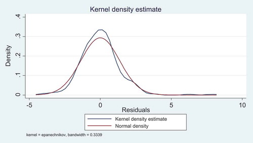
ii. Breusch-Pagan test

Breusch-Pagan/Cook-Weisberg test for heteroskedasticity

Ho: Constant variance

Variables: fitted values of HDD

chi2(1) = 6.91

Prob > chi2 = 0.0086

d. Model Specification

e. Poisson regression result

Table

Poisson regression result
	Coef.	Std. Err.	z	P>z	[95% Conf. Interval]
Diversity
Education (1= read and write)	0.0304	0.0756	0.4000	0.6870	−0.1177	0.1785
HH size (N0)	−0.0300	0.0159	−1.8900	0.0590	−0.0611	0.0012
N0 of Highest degree (M)	−0.0258	0.0504	−0.5100	0.6080	−0.1247	0.0730
N0 of Highest degree (F)	0.0770	0.0528	1.4600	0.1450	−0.0266	0.1805
Sex of HH head (1= male)	0.0680	0.3941	0.1700	0.8630	−0.7043	0.8404
Age of HH head (years)	−0.0026	0.0034	−0.7700	0.4390	−0.0092	0.0040
vocational training (1=yes)	−0.1058	0.0614	−1.7200	0.0850	−0.2261	0.0146
Working hours/day	0.0243	0.0165	1.4700	0.1400	−0.0080	0.0567
Farming experience (years)	0.0014	0.0034	0.4300	0.6680	−0.0052	0.0081
Members with farm exp (N0)	0.0264	0.0143	1.8500	0.0640	−0.0016	0.0544
Access to credit (1=yes)	0.0189	0.0532	0.3600	0.7220	−0.0853	0.1231
Residence district (1= Hurumu)	−0.1930	0.0685	−2.8200	0.0050	−0.3272	−0.0589
Land size (ha)	0.0041	0.0254	0.1600	0.8710	−0.0457	0.0540
Distance from market (minutes)	0.0003	0.0004	0.5900	0.5540	−0.0006	0.0011
Coop membership (1=yes)	−0.2008	0.3904	−0.5100	0.6070	−0.9659	0.5643
Meal frequency/day (N0)	0.1153	0.0343	3.3600	0.0010	0.0480	0.1826
Wealth rank (1=middle1)	0.0516	0.0603	0.8600	0.3920	−0.0666	0.1699
Wealth rank (1= rich)	0.1304	0.0995	1.3100	0.1900	−0.0647	0.3254
Crop species grown (N0)	0.0576	0.0260	2.2100	0.0270	0.0066	0.1086
Worry about wildlife damage (1=yes)	0.0568	0.0591	0.9600	0.3360	−0.0590	0.1727
Access to irrigation (1=yes)	−0.0414	0.0730	−0.5700	0.5700	−0.1844	0.1016
Size of home gardens (ha)	−0.2281	0.2384	−0.9600	0.3390	−0.6953	0.2391
Per capita food expenditure (log)	−0.0206	0.0245	−0.8400	0.4000	−0.0685	0.0273
Per capita nonfood expenditure (log)	0.0148	0.0240	0.6200	0.5370	−0.0322	0.0618
Constant	1.4707	0.2392	6.1500	0.0000	1.0020	1.9395

f. Ordered probit and OLS regressions re-ran replacing production diversity score with crop species count

Table

	Number of obs = 306			Number of obs =306
	LR chi2(24) =190.08			F(24, 281) =11.09
	Prob > chi2 =0.0000			Prob > F = 0.0000
Log likelihood = −193.98977	Oreded Probit model			Linear Regression Model
Diversity	Coef.	Std. Err.	z	Coef.	Std. Err.	t
Education (1= read and write)	0.1000	0.2198	0.4600	0.1255014	0.2368294	0.53
HH size (N0)	−0.1452	0.0464	−3.1300	−0.16169	0.0505606	−3.2
N0 of Highest degree (M)	−0.2532	0.1753	−1.4400	−0.149443	0.1747722	−0.86
N0 of Highest degree (F)	0.6283	0.2248	2.8000	0.5287603	0.1937833	2.73
Sex of HH head (1= male)	−0.2841	0.9201	−0.3100
Age of HH head (years)	−0.0257	0.0100	−2.5800	−0.017377	0.010766	−1.61
vocational training (1=yes)	−0.4549	0.1831	−2.4800	−0.566316	0.1963179	−2.88
Working hours/day	0.1227	0.0482	2.5500	0.1246872	0.0523024	2.38
Farming experience (years)	0.0168	0.0100	1.6900	0.0114692	0.0109091	1.05
Members with farm exp (N0)	0.1268	0.0436	2.9000	0.1489511	0.0496622	3
Access to credit (1=yes)	0.1555	0.1604	0.9700	0.1370479	0.1735893	0.79
Residence district (1= Hurumu)	−0.8723	0.2070	−4.2100	−0.903458	0.2205787	−4.1
Land size (ha)	0.0059	0.0745	0.0800	−0.008747	0.0823758	−0.11
Distance from market (minutes)	0.0006	0.0013	0.4600	0.0011355	0.0014102	0.81
Coop membership (1=yes)	−0.4081	0.9076	−0.4500	−0.681422	0.2516349	−2.71
Meal frequency/day (N0)	0.4780	0.1082	4.4200	0.6346304	0.115697	5.49
Wealth rank (1=middle1)	−0.0214	0.1747	−0.1200	0.2582532	0.1904671	1.36
Wealth rank (1= rich)	0.8624	0.3214	2.6800	0.7197032	0.3393025	2.12
Crop species count (N0)	0.1374	0.0435	3.1600	0.1648753	0.0451219	3.65
Worry about wildlife damage (1=yes)	0.3932	0.1751	2.2500	0.3065084	0.1916649	1.6
Access to irrigation (1=yes)	−0.0983	0.2124	−0.4600	−0.147332	0.2335337	−0.63
Size of home gardens (ha)	−1.1183	0.6721	−1.6600	−0.973259	0.7450237	−1.31
Per capita food expenditure (log)	−0.0861	0.0721	−1.1900	−0.10907	0.0778014	−1.4
Per capita nonfood expenditure (log)	0.0329	0.0698	0.4700	0.0735123	0.0758121	0.97
Constant				3.508991	0.7210883	4.87
/cut1	−0.6272	0.6496
/cut2	1.8937	0.6583

g: A framework for analysis of household dietary diversity

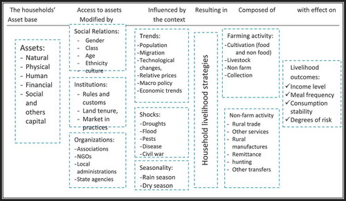
Source: Adapted from Ashley (2000)

References

- Abay, B. M., & Melese, W. A. (2019). Opportunities and challenges of adopting home garden agroforestry practices in Ethiopia: A review. Cogent Food and Agriculture, 5: 1618522, 1–29.
- Abduselam, A. M. (2017). Food security situation in Ethiopia: A review study. International Journal of Health Economics and Policy, 2(3), 86–96.
- Admassu, T. H. (2015). Population change and economic developemnt: Case studies and reflections on the ethiopian demographic transition. Developing Country Studies, 5(15), 22–37.
- Admassu, T. H., & Workneh, N. (2016). The impacts of farmer field school training on knowledge and farm technology adoption: Evidence from Smallholder Maize Farmers in Oromia, Ethiopia. Journal of Economics and Public Finance, 2(1), 1–21. doi:10.22158/jepf.v2n1p1
- Ashley, C. (2000). Applying livelihood approaches to natural resource management initiatives: Experiences in Namibia and Kenya. London: ODI.
- Babatunde, R., Omotosho, O., & Sholotan, S. (2007). Factors influencing food security status of rural farming households in North Central Nigeria. Agric J., 2(3), 351–357.
- Bank, W. (1986). Poverty and hunger: Issues and options for food security in developing countries. Washington DC: World Bank.
- Carney, D. (1999). Approaches to sustainable livelihoods for the rural poor. London: OID.
- Cordero-Ahiman, O. V., Santellano-Estrada, E., & Garrido, A. (2017). Dietary diversity in rural households: The case of indigenous communities in Sierra Tarahumara, Mexico. Journal of Food and Nutrition Research, 5(2), 86–94.
- CSA. (2011/2012). Crop Production Forecast Sample Survey Federal Democratic Republic Of Ethiopia, Central Statistical Agency. Addis Ababa: Central Statistical Agency.
- CSA. (2016). Ethiopia demographic and health survey Central Statistical Agency. Addis Ababa: Central Statistical Agency.
- Daniel, A. M., & Gerber, N. (2017). Aspirations and food security in rural Ethiopia. Food Sec., 1(9), 371–385.
- Ellis, F. (1999). Rural livelihood diversity in developing countries: Evidence and policy implications. London: OID.
- EMDHS. (2019). Ethiopia Mini Demographic and Health Survey 2019: Key Indicators. EPHI and ICF, Rockville, Maryland, USA. Addis Ababa: Ethiopian Public Health Institute.
- Fanzo, J., Marshall, Q., Wong, J., Merchan, R. I., Jaber, M. I., Souza, A., & Verjee, N. (2013). The integration of nutrition into extension and advisory services: A synthesis of experiences, lessons, and recommendations. Lindau, Switzerland: Global Forum for Rural Advisory Services.
- Fanzo, J. C. (2017). Decisive decisions on production compared with market strategies to improve diets in rural Africa. The Journal of Nutrition: Commentary, 147, 1–2. doi:10.3945/jn.116.241703
- FAO. (2007). Guidelines for measuring household and individual dietary diversity. Rome: Author.
- FAO. (2008). An introduction to the basic concepts of food security. FAO Food Security Programme. Rome: Author.
- FAO. (2010). Guidelines for measuring household and individual dietary diversity. Rome: Author.
- Greene, W. H. (2003). Econometric Analysis (5th ed.). New jersey: Prentice Hall.
- Harris-Fry, H., Azad, K., Kuddus, A., Shaha, S., Nahar, B., Hossen, M., Younes, L., Costello, A., & Fottrell, E. (2015). Socio-economic determinants of household food security and women’s dietary diversity in rural Bangladesh: A cross-sectional study. Journal of Health, Population and Nutrition, 33(2), 1–12.
- Herforth, A. (2010). Promotion of traditional african vegetables in Kenya and Tanzania: A case study of an intervention representing emerging imperatives in global nutrition. NY: Cornell University.
- Hirvonen, K., & Hoddinott, J. (2014). Agricultural production and children’s diets: Evidence from rural Ethiopia. Addis Ababa: Ethiopian Development Research Institute.
- Hoddinott, J., & Yohannes, Y. (2002). Dietary diversity as a food security indicator. Washington, DC: Food and Nutrition Technical Assistance Project (FANTA).
- IFPRI. (2017). Global food policy report. Washington, DC: International Food Policy Research Institute.
- Jemal, A., & Kim, K.-R. (2014). Determinants of household food security in rural Ethiopia: An emprical analysis. Journal of Rural Developemnt, 37(2), 129–157.
- Jones, A. D. (2017). On-farm crop species richness is associated with household diet diversity and quality in subsistence- and market-oriented farming households in Malawi. The Journal of Nutrition, 147, 86–96. doi:10.3945/jn.116.235879
- Jones, A. D., Shrinivas, A., & Bezner-Kerr, R. (2014, June). Farm production diversity is associated with greater household dietary diversity in Malawi: Findings from nationally representative data. Food Policy, 46, 1–12.
- Koppmair, S., Kassie, M., & Qaim, M. (2016). Farm production, market access and dietary diversity in Malawi. Public Health Nutrition, 20(2), 325–335. doi:10.1017/S1368980016002135
- Maddala, G. S. (1983). Limited dependent and qualitative variables in econometrics. Cambridge: Cambridge University Press.
- Mbwana, H. A., Kinabo, J., Lambert, C., & Biesalski, H. K. (2016). Determinants of household dietary practices in rural Tanzania: Implications for nutrition interventions. Cogent Food & Agriculture, 2: 1224046, 1–13.
- Muro, P. D., & Mazziotta, M. (2011). Master in human development and food security (2010/2011): Towards a Food insecurity multidimensional index (FIMI). Rome: HDFS.
- Nkegbe, P. K., Abu, B. M., & Issahaku, H. (2017). Food security in the Savannah accelerated development authority zone of Ghana: An ordered probit with household hunger scale approach. Agriculture & Food Security, 6(35), 1–11. doi:10.1186/s40066-017-0111-y
- Powell, B., Kerr, R. B., Young, S. L., & Johns, T. (2017). The determinants of dietary diversity and nutrition: Ethnonutrition knowledge of local people in the East Usambara Mountains, Tanzania. Journal of Ethnobiology and Ethnomedicine, 13(23), 1–12.
- Ruel, M. (2003). Operationalizing dietary diversity: A review of measurement issues and research priorities. The Journal of Nutrition, 133, 3911S-3926S. doi:10.1093/jn/133.11.3911S
- Scoones, I. (1998). Sustainable rural livelihoods: A framework for analysis. Brighton: IDS.
- Sibhatu, K. T., Krishna, V. V., & Qaim, M. (2015). Farm production diversity and dietary diversity in developing countries. In Agricultural & applied economics association and western agricultural economics association annual meeting (pp. 10657–10662). San Francisco: National Academy of Sciences USA (PNAS).
- Sisay, D. L., Mulugeta, D. W., & Molla, A. Y. (2019). Climate change adaptation strategies in response to food insecurity: The paradox of improved potato varieties adoption in eastern Ethiopia. Cogent Food and Agriculture, 5:1640835, 1–15.
- WFP, W. F. (2009). Emergency food security assessment handbook. Rome, Italy: United Nations World Food Programme.
- WHO. (2006). Child growth standards: Methods and development. Geneva, Switzerland: World Health Organization.
- WHO/FAO. (2003). Diet, nutrition and the prevention of chronic diseases. Geneva: World Health Organization.
- Wondimagegnhu, B. A., Admassu, T. H., & Nischalke, S. M. (2019). Determinants of farm livelihoods of smallholder farmers in Yayu biosphere reserve, SW Ethiopia: A gender disaggregated analysis. Cogent Economics & Finance, 7: 1645583, 1–19.
- Yamane, T. (1967). Statistics: An introductory analysis (2nd ed.). New York: Harper and Row.
Annex
a. Checking for MulticollinearityFootnote7