Research on the classification method of different quality dry alfalfa based on scanning electron microscopy (SEM) image texture analysis

Abstract

This study proposes a new method to distinguish between the different qualities of dry alfalfa. This method uses scanning electron microscopy (SEM) to obtain grayscale images, and. then, using an equalized histogram, the gray-level co-occurrence matrix (GLCM) extracts 14 texture features. The texture feature vector is processed by principal component analysis (PCA) and linear discriminant analysis (LDA) to reduce data redundancy and extract the best features. Finally, a back propagation neural network (BPNN) algorithm, an artificial neural network (ANN) and a least square support vector machine (LS-SVM) classification model are established to evaluate the classification effect. The results show that LDA is more effective in transforming the original data. In addition, LDA-based classification results are better than PCA-based classification results, and the recognition rate is 100% accurate. In contrast, the reliability and potential of extracting the main information based on LDA are shown. Based on these conclusions, it is possible to identify various types of alfalfa after different drying methods.

Keywords:

• scanning electron microscopy image of alfalfa
• gray-level co-occurrence matrix
• principal component analysis
• linear discriminant analysis
• classification model

PUBLIC INTEREST STATEMENT

In this study, 14 characteristic parameters were extracted by scanning electron microscopy (SEM) and the gray level co-occurrence matrix (GLCM). The distribution of 3D and 2D sampling points was studied by PCA and LDA analysis. It is most suitable for classification by LDA analysis. In addition, back propagation (BPNN) neural networks are used to compare the discriminant accuracy of different analytical methods. Artificial neural networks (ANN) are used to compare the prediction accuracy of different analytical methods. The least squares support vector machine (LS-SVM) is used to compare the classification accuracy of different analysis methods. In addition, LDA is selected according to the recognition accuracy, and the validity of LDA is verified by LDA-BPNN, LDA-ANN and LDA-LS-SVM models. The conclusion is that LDA can effectively classify alfalfa of different quality by texture analysis of scanning electron microscope images. The results show that the combination of LDA with BPNN, ANN and LS-SVM can be successfully applied to the classification of alfalfa.

Competing Interests

The authors declares no competing interests.

1. Introduction

Alfalfa is native to Persia; it is the most scattered and oldest cultivated legume forage and enjoys the reputation of the “grass crown”. This plant contains not only many important nutrients such as proteins, minerals and vitamins, but also contains essential amino acids, trace elements and unknown growth factors required by animals. Therefore, alfalfa is used as the main raw material for protein extraction and the major high-quality forage for animals. Typically, post-harvest alfalfa must be dried. Different drying methods render different characteristics and quality of the alfalfa; therefore, the classification of these different qualities is a very important research.

Traditional methods of assessment include sensory evaluation and objective measurements. The former is basically judged by experienced personnel based on the appearance of the form, while the latter usually uses physical chemistry and biological methods, such as the detection of related compounds by protein electrophoresis, gas chromatography, spectrophotometry and high-performance liquid chromatography. or detecting the number of specific spoilage organisms by microbiological analysis. These methods are relatively accurate, but always require the appropriate professionals to carry out the measurements; online identification is not possible. It is both ideal and beneficial from an economic and technical point of view to solve these shortcomings, as the reliable identification of different types of dried alfalfa is very important. Therefore, it is necessary to develop a new method to solve the limitations of traditional methods.

In recent years, with the rapid development of computer technology and machine vision, image processing has been well applied. For example, (Liu & He, 2011) black fungus producing areas were discriminated using visible/near-infrared spectroscopy and machine vision. (Tao, Wang, Li, & Qiu, 2018) used near-infrared spectroscopy and computer recognition technology to identify the sex and species of silkworm cocoons. (Zhang & Wu, 2011) researched crop classification using a forward neural network with adaptive chaotic particle swarm optimization. (Liu et al., 2012) used hyperspectral imaging and chemometrics to identify corn varieties. (Jing, Xu, Li, Li, & Liu, 2014) conducted research on the automatic classification of fabrics. (Xu et al., 2019) performed a nondestructive classification study of the apple contusion time. (Liu et al., 2018) applied infrared spectroscopy combined with computer vision technology to quickly identify triangular fan fish pearl powder using a three-step method. These studies have recognition accuracy and achieved good classification results. Therefore, in this study, a recognition method based on computer vision technology is investigated.

Although machine vision technology has been successfully applied to the identification of agriculture, there have been few reports on grass and animal husbandry. Therefore, technology has been developed to facilitate the online identification and visual classification of different drying methods to obtain the different types and qualities of alfalfa. In this study, the prepared samples were sprayed with gold and placed on a sample stage. Scanning electron microscopy (SEM) was used to capture three dry alfalfa images with different features. First, texture features were extracted using a gray-level co-occurrence matrix (GLCM). Then, principal component analysis (PCA) and linear discriminant analysis (LDA), were used to obtain the best new data combination. Finally, a back propagation neural network (BPNN) neural network, an (ANN) and a least squares support vector machine (LS-SVM) were established. The optimal classification model was obtained by comparing the performance of different classification models.

2. Materials and methods

2.1. Sample preparation

Three different kinds of dried alfalfa from the laboratory of Inner Mongolia Agricultural University, including sun dried, shade dried and mold treated alfalfa, were selected. Each sample was placed in a sealed bag of the same size (18*26 cm), and the corresponding label instruction was affixed to the bag. To meet the requirements of the sample, each sample was preprocessed before image acquisition. The method is as follows: First, a ruler was used to measure the corresponding length of the sample and the carrier at the corresponding placement site, to prevent the sample from exceeding the impact of the carrier. Next, scissors were utilized to cut off the length of the part that was needed. Finally, the two sides of the glue line were attached to the carrier to avoid falling off during the experiment. Each carrier plate was placed in 10 samples, and each drying method corresponded to 25 samples. A total of 75 samples were prepared.

2.2. Scanning electron microscopy imaging system

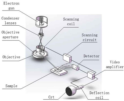
The equipment used for this experiment is shown in Figure 1. The Hitachi S-4800 field emission scanning electron microscope (S-4800 for short) was launched by Hitachi in Japan in 2002. The Hitachi S-4800 field emission scanning electron microscope is mainly composed of three basic parts: an electro-optical system, an image display and recording system and a vacuum system. The experimental system includes the following: high/low secondary electron detectors (secondary electron resolution: 1.0 nm (15 kV)/2.0 nm (1 kV)); semiconductor backscattered electron detectors (backscattered electron resolution: 3.0 nm (15 kV)); and an electron gun with a cold field emission electron source and an accelerating voltage (0.1 kV/step, variable). The system was capable of generating imagery at both low and high magnification views. The gold spray device not only makes the sample conductive but also protects the sample. The device is widely used in geology, biology, physics, chemistry and nanomaterials applications.

Figure 1. Scanning electron microscopy imaging system schematic diagram.

2.3. Image acquisition

The device was equipped with an infrared camera with a high-definition charged coupled device (CCD) of megapixels. When the acceleration voltage was selected to be low, the dispersion of the electron beam was relatively large, which reduced the resolution. Although the resolution increases as the voltage increases, when the acceleration voltage was too high, the scattering area of the sample expanded, and the intensity of the illumination increased, causing some damage to the sample. The secondary electrons on the back side caused the spots to swell. Thus, an acceleration voltage of 10 kV and a current of 10 µA was selected for the sample collection. Each image was 640 × 480 pixels, with a resolution of 600 dpi and a focal length of 30 mm. The distance between the camera lens and the sample was 7.2 mm.

2.4. Image pretreatment

Because the acquired image is a grayscale image, it is relatively dim, which has a certain influence on the calculation of the gray space matrix, resulting in poor image detail. Therefore, a histogram adjustment of the image was performed to increase the dynamic range of the gray values, thereby increasing the contrast of the entire image.

2.5. Data analysis

2.5.1. Gray-level co-occurrence matrix

Since the structure is formed by a regular distribution of the display in the spatial position, there is a grayscale relationship between the two pixels at a certain distance in image space. On the images, the gamma matrix is a common method for describing textures by studying the gray space attributes. The gray-level co-occurrence levels reflect the relative direction of the adjacent grayscale information integral space and the magnitude of changes. This level is the basis for analyzing the local patterns and the alignment of images.The image $f\left(x,y\right)$ is a two-dimensional image, S is a set of pixel pairs with a specific relationship in the R region, and the gray-level co-occurrence matrix P obtained according to the spatial relationship is:

(1) $p\left(g_1,g_2\right)=\frac{\mathrm{\#}\left\{\left[\left(x_1,y_1\right),\left(x_2,y_2\right)\right]\right\}ϵs|f\left(x_1,y_1\right)=g_1\mathrm{\&}f\left(x_2,y_2\right)=g_2}{\mathrm{\#}s}$(1)

The term on the rightside of the equation is a pair of pixels with spatial relationships; it defines the gray value as the sum, and the denominator is the sum of the pixel pairs (# represents a number).The result P is normalized.

2.5.2. Principal component analysis

PCA is the most common method for unsupervised dimensionality reduction, the extraction of high-value information, and data mapping from a high to low dimension space. Characterized by a set of original data to minimize redundancy, the main component is used to maximize the information extracted feature set. All of the information is combined in a new combination of variables. For example, raw data may be very dense in one dimension; PCA is able to find an axis or a place where dimensionality can be reduced. The diffusion of dense points is relatively large for each point distribution. This process is equivalent to finding the direction of the largest variance because the direction of the largest variance will render the points less diffuse after PCA dimensionality reduction. It is better to carry out the classification tasks. From the point of view of the process, first find the covariance matrix, find the eigenvalue, then find the eigenvalue corresponding to the largest eigenvector, return it to the original data to obtain the dimension reduction results.

2.5.3. Linear discriminant analysis

LDA is a supervised algorithm. In 1936, Fisher first proposed the second classification problem, also referred to as the Fisher linear discrimination. The idea of linear discrimination is very simple: provide some training examples, and attempt to design the samples in a straight line so that the design points of the same sample type are as close as possible (the design points of different samples types are as far away from each other as possible). Design in the same row and specify a new sample category based on the position of the projected point during categorization. The algorithm flow is as follows: Input: Dataset $D=\left\{\left(x_1,y_1\right),\left(x_2,y_2\right),\dots ,\left(x_m,y_m\right)\right\}$, each sample $x_i$ is an n-dimensional vector, $y_i\in \left\{C_{1,}{C}_2,\dots ,C_k\right\}$ the dimension is reduced to dimension $d.$

1. Calculate the intraclass divergence matrix $S_w$

2. Calculate the intraclass divergence matrix $S_b$

3. Calculation matrix $S_w^{-1}$

4. Calculate the maximum deigenvalues of $S_w^{-1}{S}_b$ and corresponding deigenvectors $\left(w_1,w_2,\dots ,w_d\right)$ to obtain the projection matrix $W$

5. Convert each sample feature $x_i$ in the sample set to a new sample $z_i=W^T{x}_i$

6. Obtain the output sample set $D^{,}=\left\{\left(z_1,y_1\right),\left(z_2,y_2\right),\dots ,\left(\left(z_m,y_m\right)\right)\right\}$

2.5.4. BPNN

The BPNN is an algorithm for learning with neural networks. The network consists of three layers: input, intermediate, and output. The intermediate layer can extend to multiple layers. The neurons in adjacent layers are completely interconnected, and there is no connection between the neurons in each layer. When a pair of learning modes is passed to the network, each neuron receives an input network response to generate a weight for the connection, reduce the direction of the desired output and the actual output error, correct each connection layer from each layer of the output layer through each intermediate layer, go to the input graph, and repeat the process alternately. When the global network error approaches the minimum the learning process is over.

2.5.5. Artificial neural network

An artificial neural network consists of a series of layers, with each layer containing a set of neurons. All layers of a neuron are associated with a particular weight. Actually, it is a complex network with a large number of simple connected components and a high degree of nonlinearity;the system is capable of performing complex logic operations with nonlinear relationships. The structure of the ANN specifies the variables in the network and their topological relationships. The neural network variables can be neuron connection weights as well as neuron excitation values. Most neural network models have a short-term dynamics rule that determines how neurons change their stimulus values based on the activity of other neurons. The overall incentive function depends on the weight of the network. The network’s learning rules dictate how the weights in the network adjust over time, which is often seen as a dynamic rule for long-term scales. In general, the learning rules depend on the excitation values of the neurons and may also depend on the target value and current weight value provided by the supervisor.

2.5.6. Least squares support vector machine

The support vector machine (SVM) is a general method of machine learning based on statistical learning theory. It is a learning system that uses a space of a hypothetical linear function in a higher dimensional space. This method is also a suitable way to solve finite groups and is able to handle complex nonlinear problems. The main technique of the support vector machine is the application of the kernel function. That is, the nonlinear segmentation problem, which is difficult to solve in the dimension space, is mapped to the high-dimensional space by the hierarchical method, although an increase in the spatial dimension increases the computational complexity in some way. However, using the kernel function can transform the nonlinear problem into a linear problem, which is a good solution to the problem of dimensional increase and computational complexity. The LS-SVM is a further improvement of the SVM algorithm. The least squares method selects the hyperplane from the square of the error and establishes the squared loss function. At the same time, the SVM inequality constraint is transformed into a linear equation, which solves the quadratic programming problem. This method converts to a faster, more efficient linear solution algorithm than the SVM. Choosing the right kernel function and parameters is the key to the success of the LS-SVM. The radial basis function (RBF) is a high-performance kernel function. The choice of core parameters and penalty factors (γ，∁) determines the performance of the SVM classification. Therefore, this work chose the RBF kernel function.

PCA, LDA and BPNN data analysis were conducted in IBM SPSS 25, and ANN and LS-SVM analyses were performed in MATLAB R2018a (MathWorks, Natlick, Mass.) software.

3. Results and discussion

3.1. Image pretreatment

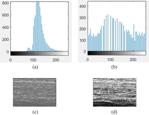
In this paper, the experimental samples used three types of alfalfa images: sun dried, shade dried and mold treated images. First, the image is histogram equalized and can be displayed to extract more information regarding the structure of the image. The pretreatment results of the sun-dried alfalfa are shown in Figure 2.

Figure 2. Comparison of the images and histograms of the gray images processed by histogram equalization (a) Histogram gray alfalfa image of the original image (b) Enhanced histogram of the alfalfa image (c) Gray alfalfa image (d) Enhanced alfalfa image.

3.2. Texture feature extraction

Under the GLCM, various structural features, such as entropy, energy, correlation and contrast, of the alfalfa SEM image can be extracted. This paper referred to a large number of references worldwide (Clausi, 2002; Haralick, Shanmugam, & Dinstein, 1973; Soh & Tsatsoulis, 1999) to obtain multiple texture parameters based on SEM images. To reduce the redundancy and improve the accuracy of classification, fourteen texture parameters were selected, as shown in Table 1. These fourteen parameters were used to describe image features and, extract image texture features.

Table 1. Definition of each texture feature parameter

Parameter	Formula
Contrast	$f_1=\sum _{n=0}^{N_g-1}{n}^2\left\{\sum _{i=1}^{N_g}\sum _{j=1}^{N_g}p\left(i,j\right)\left|i-j\right|=n\right\}$
Correlation	$f_2=\frac{{\sum }_i{\sum }_j\left(i,j\right)p\left(i,j\right)-{\mu }_x{\mu }_y}{{\sigma }_x{\sigma }_y}$
Prominence of Clustering	$f_3=\sum _i\sum _j{\left(i+j-{\mu }_x-{\mu }_y\right)}^{4}p\left(i,j\right)$
Shadow of Clustering	$f_4=\sum _i\sum _j{\left(i+j-{\mu }_x-{\mu }_y\right)}^{3}p\left(i,j\right)$
Angular Second Moment	$f_5=\sum _i\sum _j{\left\{p\left(i,j\right)\right\}}^2$
Entropy	$f_6=-\sum _i\sum _{j}p\left(i,j\right)log\left(p\left(i,j\right)\right)$
Inverse Difference Moment	$f_7=\sum _i\sum _j\frac{1}{1+\left(i-j\right)}p\left(i,j\right)$
Maximal Probability	$f_8=\begin{array}{c}\mathrm{M}\mathrm{A}\mathrm{X}\\ i,j\end{array}p\left(i,j\right)$
Sum of Squares Variance	$f_9=\sum _i\sum _j{\left(i-\mu \right)}^{2}p\left(i,j\right)$
Sum of Average	$f_{10}=\sum _{i=2}^{2N_g}i{p}_{x+y}\left(i\right)$
Sum of Variance	$f_{11}=\sum _{i=2}^{2N_g}{\left(i-f_8\right)}^2{p}_{x+y}\left(i\right)$
Sum of Entropy	$f_{12}=-\sum _{i=2}^{2N_g}{p}_{x+y}\left(i\right)log\left\{p_{x+y}\left(i\right)\right\}$
Variance of Difference	$f_{13}=varianceof{p}_{x-y}$
Difference of Entropy	$f_{14}=-\sum _{i=0}^{N_g-1}{p}_{x-y}\left(i\right)log\left\{p_{x-y}\left(i\right)\right\}$

3.2.1. PCA using image data

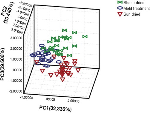
PCA was applied to all image data obtained from all samples to reduce high dimensions and check for qualitative differentiation in the different dried images. The variance rates of the first three principal components of the interpretation are 32 336%, 30.440% and 29.506% of the total, indicating that the accumulation of the first three components can explain 92.282% of the overall information, so it can be used to indicate the classification of all variables. To interpret the PCA results, scoring is typically performed by visualizing their PCs. Figure 3 shows the PC1 × PC2 × PC3 score plot for all of the samples. Different dry alfalfa samples are separately distributed in the three-dimensional region depending on the color and shape of each variety. Although the sample varieties are gathered separately, their boundaries are not clear, because some sample point edges overlap.It is difficult to distinguish the scores of different sample results in the three-dimensional region. Therefore, more classifiers are needed based on the PCA process.

Figure 3. Cluster diagram of each different quality of dry alfalfa.

3.2.2. LDA using image data

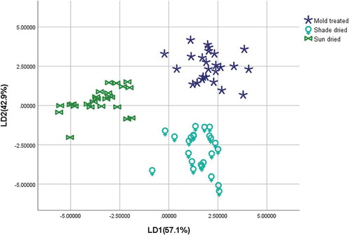
Similarly, LDA was used for all images. As shown in Figure 4, the score maps of the two discriminant functions were extracted. The score of the first discriminant function is 61.6%, the score of the second discriminant function is 38.4%, and the cumulative change of the two reaches is 100%. The cumulative change over PCA exceeded 7.718%. From a graphical point of view, the three types of classifications are more obvious, and the boundaries are not overlapping. This method shows that the first two functions extracted can also represent the overall information, while the LDA extraction function is better than traditional PCA.

Figure 4. Score diagram of the two discriminant functions.

3.3. Classification results

3.3.1. BPNN model

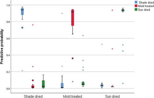
The PCA-based BPNN model and the BPNN model were established by the selected PCs. The first three PCs were used as input variables; the number of input layer units was 3; the number of hidden layers was 1; the number of units was 2; the hidden layer activation function was a hyperbolic tangent function; the number of output layer units was 3; and the activation function was a softmax function. The initial value of lambda was 0.0000005, the initial value of sigma was 0.00005, and the interval offset was ±0.5. The classification results are shown in Table 2. In the training samples, the correct rate of shade drying was 94.4%, the correct rate of sun drying was 93.8%, the correct rate of mold treatment was 86.7%, and the overall correct percentage was 91.8%. In the testing samples, the correct rate of shade drying was 100%, while the correct rate of sun drying was 75.0%, and the correct rate of mold treatment was 100%. In the verified samples, the overall correct rate was 90.9%, and the whole model was relatively good. From Figure 5, it was found that the probability of selecting shade dried samples in the shade dried samples was over 90%, and the probability of selecting sun dried and mold treatment in the shade dried samples was relatively low. In the sun dried samples, the probability of selecting sun dried samples was also over 90%, and the probability of selecting shade dried and mold treatment was relatively low. In the mold treatment samples, the probability of selecting mold treatment samples was close to 90%, and the correct rate of selecting shade dried samples was relatively higher.

Table 2. Classification accuracy rate

Sample	Measured	Shade dried	Sun dried	Mold treatment	Correct percentage
Train	Shade dried	17	0	1	94.4%
	Sun dried	0	15	1	93.8%
	Mold treatment	1	1	13	86.7%
	Overall percentage	36.7%	32.7%	30.6%	91.8%
Calibration	Shade dried	3	0	0	100.0%
	Sun dried	1	6	1	75.0%
	Mold treatment	0	0	4	100.0%
	Overall percentage	26.7%	40.0%	33.3%	86.7%
Validation	Shade dried	3	0	1	75.0%
	Sun dried	0	1	0	100.0%
	Mold treatment	0	0	6	100.0%
	Overall percentage	46.7%	20.0%	33.3%	100.0%

Figure 5. Observation forecast chart.

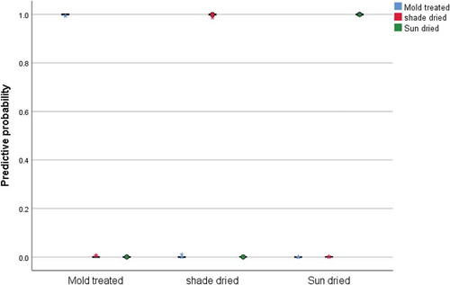
For the LDA-based BPNN model, 60% of the samples were randomly selected for training, 20% were used as test samples, and 20% were used as verification samples. The classification results are shown in Table 3. For training, test or verification samples, the correct rate of prediction was 100% of all samples, and the correct rate of prediction for each type was also 100%. It can be seen from Figure 6 that in the shade dried samples, the probability of selecting shade dried samples was 100%, the probability of selecting sun dried and mold treatment samples was 0%. In the sun dried samples, the probability of selecting sun dried samples was 100%, the probability of selecting shade dried and mold treatment samples was 0%. In the mold treatment samples, the probability of selecting mold treatment samples was 100%, and the probability of selecting shade dried and sun dried samples was 0%. It can be seen that the LDA-based BPNN model achieves 100% accuracy with regard to the classification results.

Table 3. Classification results

Sample	Measured	Shade dried	Sun dried	Mold treatment	Correct percentage
Train	Shade dried	13	0	0	100.0%
	Sun dried	0	13	0	100.0%
	Mold treatment	0	0	12	100.0%
	Overall percentage	34.2%	34.2%	31.6%	100.0%
Calibration	Shade dried	5	0	0	100.0%
	Sun dried	0	9	0	100.0%
	Mold treatment	0	0	8	100.0%
	Overall percentage	22.7%	40.9%	36.4%	100.0%
Validation	Shade dried	7	0	0	100.0%
	Sun dried	0	3	0	100.0%
	Mold treatment	0	0	5	100.0%
	Overall percentage	46.7%	20.0%	33.3%	100.0%

Figure 6. Observation forecast chart.

3.3.2. ANN model

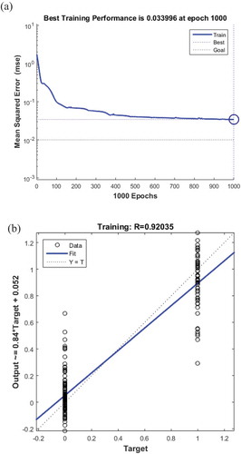
For the PCA-based ANN model, a three-layer network of the input layer, hidden layer and output layer was established, 60 samples were randomly selected for training, and the remaining samples were used for testing. The learning rule used a gradient descent adaptive training function with a maximum number of iterations of 1000. The results are shown in Figure 7(a,b). The network training reached convergence after approximately 130 iterations, and the correlation coefficient was 0.92035. As shown in Table 4, the correct recognition rate was 93.33%. It can be seen that the recognition result of the model was quite impressive. It can provide a reference value for engaging in the classification and grading of pasture products.

Table 4. Identification results of each model

Model	Recognition(%)
PCA-ANN	93.33
LDA-ANN	100
PCA-LS-SVM	86.667
LDA-LS-SVM	100

Figure 7. PCA input results of the ANN model (a) Network training error curve (b) Schematic diagram of the neural network output value and target value comparison.

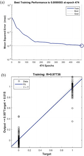
For the LDA-based ANN model, a three-layer network was established. The hidden layer neuron activation function was logsig, the output layer neuron activation function was purein, the number of learning times was set to 1000, and the training time of the network was 0.03 seconds. The training result is shown in Figure 8(a,b). The network training reaches convergence after approximately 150 iterations. When training to step 474, the training stops in advance; at this time, the network error was 0.0099503, and the correlation coefficient was 0.97736. Table 4 shows that the correct recognition rate reached 100% of the prediction accuracy, and the classification effect was quite good, which can provide an effective tool for the classification of different qualities of dry alfalfa.

Figure 8. LDA input results of the ANN model (a) Network training error curve (b) Schematic diagram of the neural network output value and target value comparison.

3.3.3. LS-SVM model

By classifying the samples using the LS-SVM model, since the performance of the SVM model is influenced by the parameter settings, the penalty factor and the kernel function were optimized. To obtain accurate results, a “grid” search of different parameters was applied, and the best combination of the two parameters was determined by cross validation. The parameters that yield the best classification accuracy for the model are shown in the classification diagram.

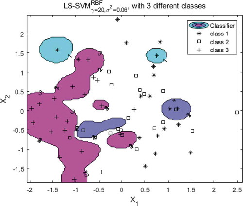
For the PCA-based LS-SVM model, the classification results are shown in Figure 9. The first type of sun-dried alfalfa sample points were arranged in a longitudinal direction, spread out from the middle up and down. The second type of shade dried alfalfa sample points were arranged in a horizontal direction, and the middle was dense. The two types of sample points were mixed and distributed, so the classification effect was not ideal. The distribution of the third mold treatment alfalfa sample points was independent and slightly mixed with the other two boundaries, and the distribution was relatively concentrated in general. The model based on PCA-LS-SVM provided an 86.667% recognition rate, as shown in Table 4. From the picture, many sun-dried and shade- dried alfalfa samples were misclassified. Overall, the classification effect was not ideal.

Figure 9. Classification results.

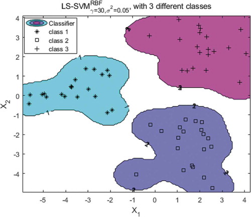
For the LDA-based LS-SVM model, the classification results are shown in Figure 10. Three different dry alfalfa samples were randomly distributed, and each type of alfalfa was concentrated and arranged in a concentrated manner; no mixing occurred. The LDA-based LS-SVM model, as shown in Table 4, provided a 100% recognition rate, which was very satisfactory. Therefore, the LDA-LS-SVM model can effectively distinguish the types of different dry alfalfa without misclassification. which can be a tremendous benefit for grass husbandry.

Figure 10. Classification results.

4. Conclusion

This study proposes a new method for the online identification of different quality dry alfalfa. First, GLCM was used to extract the pretreatment image features. Second, PCA and LDA were used for data reduction to obtain the main features. Finally, three different dry alfalfa were identified by a neural network. The highest recognition accuracy of the three models based on PCA is 93.33%. The LDA-based BP, ANN and LS-SVM models demonstrate a higher recognition accuracy than the three models based on PCA. Satisfactorily, the accuracy is 100%. The results show that the classification accuracy of the LDA-based classification model is better than that of the PCA-based classification model, which shows that the information extracted by LDA is more effective; meanwhile, the model is also optimized. These promising indications can provide a reference for the industry classification of alfalfa.

Additional information

Funding

This study was supported by the National Natural Science Foundation of China (Project No: 61265011), Inner Mongolia Natural Science Foundation (Project No: 2018MS06012), Research Fund for the Doctoral Program of Higher Education (Project No: 20111515120004).

Notes on contributors

Guifang Wu

I am working in the agricultural and animal husbandry technology innovation research group, and the research group is mainly engaged in the intelligentized approach to agricultural and livestock equipment, post-harvest processing of agricultural and livestock products, optimization of the production environment for agriculture and animal husbandry, and research on informatization of agriculture and animal husbandry. The projects we are currently working on are the following: The National Natural Science Foundation: Study on Detection of Cashmere Qualities Based on Information Fusion of Near Infrared Spectroscopy and Field Emission Scanning Electron Microscope Image, and the Inner Mongolia Science Fund: Research on Quality Detection of Alfalfa Based on Multi-sensor Information Fusion. The main content of this article is part of the Inner Mongolia Science Fund.

References

- Clausi, D. A. (2002). An analysis of co-occurrence texture statistics as a function of grey level quantization. Canadian Journal of Remote Sensing, 28(1), 45–15. doi:10.5589/m02-004
- Haralick, R. M., Shanmugam, K., & Dinstein, I. (1973). Textural features for image classification. IEEE Transactions on Systems Man Cybernetics-Systems, 3(6), 610–621. doi:10.1109/TSMC.1973.4309314
- Jing, J., Xu, M., Li, P., Li, Q., & Liu, S. (2014). Automatic classification of woven fabric structure based on texture feature and pnn. Fibers and Polymers, 15(5), 1092–1098. doi:10.1007/s12221-014-1092-0
- Liu, F., & He, Y. (2011). Discrimination of producing areas of auricularia auricular using visible/near infrared spectroscopy. Food and Bioprocess Technology, 4(3), 387–394. doi:10.1007/s11947-008-0174-7
- Liu, S., Wei, W., Bai, Z., Wang, X., Li, X., Wang, C., … Xu, C. (2018). Rapid identification of pearl powder from hyriopsis cumingii by Tri-step infrared spectroscopy combined with computer vision technology. Spectrochimica Acta Part A-Molecular and Biomolecular Spectroscopy, 189, 265–274. doi:10.1016/j.saa.2017.08.031
- Pan, X. Y., Sun, L. J., Li, Y. S., Che, W. K., Ji, Y. M., Li, J. L., Li, J., Xie, X., & Xu, Y. T. (2019). Non-destructive classification of apple bruising time based on visible and near-infrared hyperspectral imaging. Journal of the Science of Food and Agriculture, 99(4), 1709–1718. doi: 10.1002/jsfa.9360
- Soh, L. K., & Tsatsoulis, C. (1999). texture analysis of sar sea ice imagery using gray level co-occurrence matrices. IEEE Transactions on Geoscience and Remote Sensing, 37(21), 780–794. doi:10.1109/36.752194
- Tao, D., Wang, Z., Li, G., & Qiu, G. (2018). Accurate identification of the sex and species of silkworm pupae using near infrared spectroscopy. Journal of Applied Spectroscopy, 85(5), 949–952. doi:10.1007/s10812-018-0744-z
- Zhang, X. L., Liu, F., He, Y., & Li, X. L. (2012). Application of hyperspectral imaging and chemometric calibrations for variety discrimination of maize seeds. Sensors, 12(12), 17234–17246. doi: 10.3390/s121217234
- Zhang, Y., & Wu, L. (2011). Crop classification by forward neural network with adaptive chaotic particle swarm optimization. Sensors, 11(5), 4721–4743. doi:10.3390/s110504721