Welfare and food security effects of commercializing African indigenous vegetables in Kenya

Abstract

African indigenous vegetables (AIVs) have high nutritional value, forming a potent weapon against the pressing hidden hunger problem in East Africa, but they are not sufficiently adopted as cash crops by Kenyan small-scale farmers to meet the rising demand in the urban areas. This study therefore aims (i) to explore which factors motivate small-scale farmers to specialize in commercial AIV production and (ii) to assess the impact of AIV production on household income and food security. This analysis was based on primary data from 706 rural and peri-urban small-scale vegetable producers in Kenya. Results of a binary choice model showed that education, participation in producer groups, access to market information and irrigation water, as well as distance to the next city influenced the decision to commercialize AIV production. Impact analysis was conducted with binary and continuous propensity score matching (PSM) and endogenous switching regression (ESR). The production of AIVs as cash crops positively influenced the total per capita household income and the food security status of the households.

Keywords:

• African indigenous vegetables
• food security
• household income
• propensity score matching
• endogenous switching regression
• East Africa

PUBLIC INTEREST STATEMENT

Despite great effort of policy makers and NGOs, micronutrient deficiency still remains a significant problem in Kenya. African indigenous vegetables (AIVs) are very high in micronutrients and can thus play an important role in combating micronutrient deficiency in the Kenyan population. In the last decade, the demand for AIVs in the urban areas has been constantly increasing. However, supply is lagging behind because of reluctant commercialization of those crops by Kenyan farmers in rural and peri-urban areas. With a survey of Kenyan small-scale farmers in rural and peri-urban areas in Kenya, we discover adoption patterns of commercial AIV production. Further, we find that commercial AIV production indeed increases household income and food security status of the households. Policy makers and agricultural extension officers should thus focus on those crops to increase economic development and combat malnutrition in rural and peri-urban areas in Kenya.

Competing Interest

The authors declare no competing interest.

1. Introduction

African Indigenous Vegetables (AIVs) have been widely used for subsistence farming in East Africa for thousands of years. In the last decade, however, rural-urban migration and a shift in consumer preferences has led to an increased demand for commercially marketed AIVs. This trend was spurred by the increasing recognition of the high nutritional value of AIVs (Cernansky, 2015), which offer a solution to the region’s pressing problem of micronutrient deficiencies—the so-called hidden hunger problem. Despite great national and international efforts, hidden hunger remains a chronic issue in East Africa. In Kenya alone, almost one-third of all children show retarded physical development due to micronutrient deficiencies (WFP, 2018).

63 % of agricultural output in Kenya is still generated by small-scale farmers who are simultaneously producers and consumers (Rapsomanikis, 2015). Based on the current literature, we hypothesized that Kenyan small-scale farmers benefit from growing these traditional crops as cash crops in two ways. First, they benefit economically from a rising market, and second, they benefit in terms of food security because they can consume the nutritious vegetables themselves. Studies estimating the actual impact of the production of AIVs on income are scarce. The existing studies (Ewbank, Nyang, Webo, & Roothaert, 2007; Gotor & Irungu, 2010) were conducted during the course of AIV introduction and market development programmes and thus potentially overstated the positive effect of growing AIVs. Most of the current literature linking AIVs to food security only investigated the nutrient content of the AIVs to draw conclusions on their potential to combat food insecurity (Faber, van Jaarsveld, & Laubscher, 2009; Legwaila, Mojeremane, Madisa, Mmolotsi, & Rampart, 2011; Msuya, Mamiro, & Weinberger, 2009). A high nutrient content itself, however, does not guarantee the sufficient nutrient intake of the producing households. This study therefore aimed to fill this gap by analysing the actual impact of the production of AIVs as cash crops on household income and the impact of their production as staple crops on food security status.

The study at hand is based on cross-sectional data with 706 observations from four counties in rural and peri-urban Kenya. Based on a probit regression choice model, we discuss factors that determine the focus on commercial AIV production. As AIVs, we focus on amaranth (Amaranthus spp.), cowpea (Vigna unguiculata), African nightshade (Solanum spp.) and spider plant (Cleome gynandra), which are economically the top four AIVs grown in Kenya (Abukutsa-Onyango, 2010). Propensity score matching (PSM) and endogenous switching regression (ESR) were used to reduce self-selection bias and pinpoint the effect of the focus on commercial AIV production on household income and food security. For the analysis, we used two different definitions of commercialization. First we investigate the binary case of whether or not households sell their AIV production; then we look at the effects of different intensities of commercialization depending on how much of the harvest was sold to the market (Omiti, Otieno, Nyanamba, & McCullough, 2009). We used various food security indicators to give a more comprehensive picture of the importance of AIVs for food security. These indicators covered the four different dimensions of food security (FAO, 2008): availability, accessibility, stability and utilization.

The article is structured as follows: First, we provide an overview of the literature to build the conceptual framework and argue for the selection of outcome variables and explanatory variables. A description of the data and methodology used follows. In the results section, we present and discuss descriptive and econometric results of this choice and impact models. The article concludes with the implications of the results for policy makers and further research.

2. Literature review

2.1. Potential of AIVs in Kenya

AIVs, most of which are leafy vegetables cooked prior to consumption, have been grown and consumed in East Africa for thousands of years. Based on their economic and nutritional potential, amaranth (Amaranthus spp.), cowpea (Vigna unguiculata), African nightshade (Solanum spp.) and spider plant (Cleome gynandra) are the top four AIVs grown in Kenya, Tanzania and Uganda (Abukutsa-Onyango, 2010). Those four varieties are the most cultivated AIVs by small-scale vegetable producers in eastern and central Kenya (Mbugua et al., 2011), but there are many more varieties consumed and cultivated in areas where research and strategies for commercialization are still very limited.

While they have long been slighted as “poor people’s food” or “famine food” (Mbhenyane, Venter, Vorster, & Steyn, 2016; Weinberger & Msuya, 2004), the presence of AIVs in Kenya’s urban markets has significantly increased since the 2000s. The main reason for this is growing consumer demand due to the nutritional benefits of these crops (Irungu, Mburu, Maundu, Grum, & Hoeschle-Zeledon, 2007). AIVs are now even served in some expensive restaurants in Nairobi (Cernansky, 2015), and end customers show a significant willingness to pay higher prices for high quality AIVs (Croft, Marshall, & Weller, 2014).

Increasing numbers of producers have responded to this trend in the last decade and engaged in AIV production and marketing (Gotor & Irungu, 2010). Because AIVs are perishable and cooled storage is not usually available, AIVs for the urban market are produced in or very close to cities (Weinberger & Pichop, 2009). The area under cultivation with AIVs in Kenya grew by 25% between 2011 and 2013 (Cernansky, 2015). The production of these crops can be beneficial for small-scale farmers since they can obtain higher prices compared to those obtained for exotic vegetables (Ndenga, Achigan-Dako, Mbugua, Maye, & Ojanji, 2013; Weinberger & Pichop, 2009).

2.2. Adoption of commercial AIV production

Constraining factors for the adoption of commercial AIVs are a lack of knowledge about cultivation, processing and marketing and a lack of market information (Ayodele, Makaleka, Chaminuka, & Nchabeleng, 2011; Mbugua et al., 2011). Access to information about commercial AIV production decreases with the increasing distance from Nairobi (Gotor & Irungu, 2010). In rural eastern and central Kenya, the lack of knowledge of the plants and their preparation by consumers is a major constraint to the adoption of commercial AIV production. Many AIVs are considered weeds and inferior to exotic cabbage (Mbugua et al., 2011). In the case of rural South Africa, older people know more about AIV production and consumption than the younger population, although this knowledge is for subsistence farming only (Modi, Modi, & Hendriks, 2006).

Access to extension services facilitates commercial AIV adoption in Kiambu because they offer improved and more profitable varieties of AIVs (Ewbank et al., 2007; Mwaura, Muluvi, & Mathenge, 2013). The more producers there are that already specialize in crop production, the more likely they are to adopt commercial AIV production (Gotor & Irungu, 2010). Indeed, producer groups can be very beneficial for the adoption process since farmers can obtain additional information. Producer groups have also been found to catalyse the adoption of new agricultural technologies and trends (Asfaw, Mithöfer, & Waibel, 2010; Ngokkuen & Grote, 2012). Furthermore, those who adopt new technologies are often more socially active than those who do not (Rogers, 2003).

Higher formal education increased commercialization levels among Kenyan small-scale farmers kale and maize (Omiti et al., 2009). In contrast, AIV producers generally had lower levels of education that did not reach far above primary education (Weinberger & Pichop, 2009).

For leafy vegetables such as AIVs, it is very beneficial to provide irrigation during the dry season because a steady water supply can increase the yield, quality and uniformity of the harvest (Fereres, Goldhamer, & Parsons, 2003). In this way, irrigation measures have increased the profitability of horticultural crops in semi-arid regions (Kuşçu, Çetin, & Turhan, 2009; Mwangi & Crewett, 2019). The irrigation of AIV cultivations increased the marketing potential of AIV producers in Kiambu County (Mwangi & Crewett, 2019). However, irrigation technology is often not available for AIV farmers, mainly because of a lack of capital to invest in those measures (Ewbank et al., 2007). Although investment capital and liquidity are very important in the seasonal business of agriculture, Kenyan AIV farmers often face problems in obtaining basic financial services (Mwaura et al., 2013).

Despite the constraints on capital and technology, it is relatively easy for households with poor physical and natural asset endowments to specialize in commercial AIV production because they need less input to start with than those wo grow other cash crops (Ayodele et al., 2011; Gockowski, Mbazo’o, Mbah, & Fouda Moulende, 2003), and the farmers can work on very small plots of land (Gockowski et al., 2003; Weinberger & Msuya, 2004).

The gender of the head of the household seems to play a role in the adoption of commercial AIV production. Although most Kenyan AIV producers are female, the share of men in AIV production is significantly higher in urban areas than that in rural areas. (Weinberger & Pichop, 2009) explained this to be the result of a more intense production and the shift of AIVs as a subsistence crop to a cash crop in urban areas. In Kenya, women are traditionally responsible for cultivating subsistence crops, with men responsible for cultivating for cash crops.

2.3. Effect of growing AIVs on food security and income

Food security is a complex issue that cannot be measured by one indicator alone. In this analysis, we used the definition of food security from the Food and Agriculture Organization of the United Nations (FAO), in which food security is divided into four dimensions: physical availability of food, economic and physical access to food, food utilization and the stability of these three dimensions over time (FAO, 2008).

Physical availability refers to the supply side of food security in terms of food production, stocks and imports, which still do not meet the minimum requirements for the Kenyan population (WFP, 2018). Since Kenyan small-scale farmers are both producers and consumers, their agricultural output enhances the availability of food, especially if markets are not sufficiently developed (FAO, IFAD, & WFP, 2013).

The access dimension of food security addresses the availability of food on the household level. It can be enhanced by a higher household income, lower food prices or better functioning markets (FAO, 2008). In rural areas, AIVs are very nutrient rich and can be bought for relatively low prices. This is why poorer households in rural areas receive a great share of their nutrients from AIVs (Gockowski et al., 2003; S. Singh, Singh, Singh, Chand, & Roy, 2013; Weinberger & Msuya, 2004). Growing and marketing AIVs can increase the net gains per acre and reduce the level of poverty for households situated in peri-urban Kiambu County (Ewbank et al., 2007; Gotor & Irungu, 2010). However, those results were generated as part of dissemination programmes and were potentially overstated. In rural Tharaka County, where the market for AIVs is not as developed as that in peri-urban areas, the growth of AIVs for commercial purposes actually increased poverty levels (Gotor & Irungu, 2010). Despite those indistinct results on the effect of AIV growth on income, several authors stressed the strong potential of AIVs to lift small-scale farmers out of a condition of malnutrition and poverty (Cernansky, 2015; Ndenga et al., 2013; Weinberger & Pichop, 2009).

The strong potential of AIVs to enhance food utilization is well documented. The utilization dimension of food security involves micronutrient content, food diversity, the distribution of food within the household and how the body makes use of nutrients (FAO, 2008). Due to their high levels of micronutrients, AIVs are a very suitable tool to fight so-called “hidden hunger” (Msuya et al., 2009). “Hidden hunger” describes a state in which people consume enough calories but do not have enough nutrients available, and it is a very common problem in Kenya (Muthayya et al., 2013). Dark green, leafy vegetables can substantially contribute to the intake of calcium, iron, vitamin A and riboflavin, especially in young children (Faber et al., 2009). Amaranth in particular contains very high levels of calcium, magnesium and zinc, and African nightshade has a high potassium and iron concentration (Kamga, Kouamé, Atangana, Chagomoka, & Ndango, 2013). In particular, accessibility to iron is enhanced through the proper preparation of AIVs through boiling and frying (Habwe, Walingo, Abukutsa-Onyango, & Oluoch, 2009). The protein content of AIVs can reach up to 36% (Legwaila et al., 2011) and is thus substantially higher than that of kale or spinach, which are currently consumed on a large scale in Kenya.

The stability dimension of food security describes the stability of the other dimensions over time (FAO, 2008). AIVs perform well in this dimension because they are still available when food from crop production is scarce (Modi et al., 2006). In the dry regions of Tanzania, AIV subsistence production is used to compensate for shortages in the dry season (Weinberger & Msuya, 2004).

3. Data and methodology

3.1. Data

This study is based on data from the HORTINLEA¹ household survey (2015). The survey took place at the end of September until the beginning of December, 2015 and thus fell in the beginning of the short rainy season.

A total of 706 households were selected with a multi-stage sampling technique. First, four counties (Kisii, Kakamega, Kiambu and Nakuru) were selected because of the high prevalence of AIV production in these counties. The study site in Kiambu is close to the city of Nairobi, while the site in Kakamega is relatively close to Kisumu (Figure A1 in appendix A). With the help of district agricultural offices, we determined the districts in these four counties in which AIV production is concentrated. From each of the selected districts, we randomly sampled locations/wards. Farmers within those locations were randomly selected based on household lists from agricultural extension officers. The distribution of the samples among counties is shown in Table 1.

Table 1. Geographic distribution of samples via counties

AIV commercialization	Kisii	Kakamega	Nakuru	Kiambu	Total
Household (HH) sells AIVs	130	157	81	121	489
HH does not sell AIVs	71	45	70	31	217
Total	201	202	151	152	706

The questionnaire covers all sources of livelihood and farm activities at the households ranging from sociodemographic characteristics, occupations, agricultural production and marketing to food and non-food consumption, food security and shocks. The food consumption section consists of a detailed one-week summary of all types of food eaten, including their quantities and prices. Furthermore, remittances, all agricultural and household assets, and rented and owned land holdings are included in the questionnaire.

3.2. Theoretical and conceptual framework

According to the sustainable livelihood framework, households will try to maximize their utilization given the resources they have available and will engage in a set of activities to form a livelihood strategy (DFID, 1999; Scoones, 1998). One of these activities can be commercial AIV production (Figure 1).

Figure 1. Process to adopt commercial AIV production and its influence on livelihood outcomes.

Note: Source: own construction based on (DFID, 1999; Hartje, Bühler, & Grote, 2018; Scoones, 1998).

For the analysis, we assumed that households will rationally try to maximize their utility from the consumption of goods produced on the farm ($c_m$), products bought in the market ($r_m$) and leisure time ($l_i$) (Equation 1 based on Asfaw et al., 2010; Singh, Squire, & Strauss, 1986). Exogenous factors such as shocks and public infrastructure ($T_u$) can influence the following utility function (Asfaw, Shiferaw, Simtowe, & Lipper, 2012; DFID, 1999; Scoones, 1998):

(1) $U=u\left(c_m,r_m,l_i;T_u\right)$(1)

When making a decision on livelihood activities, the household faces a cash income, time and technology constraint (Asfaw et al., 2012; I. Singh et al., 1986). Since focusing on commercial AIV production would lead to the specialization of the household and restrain significant resources in terms of labour and farm input, we assumed that labour and farm input are functions of the adoption of commercial AIV production. The household will thus pursue commercial AIV production if the marginal benefits of AIV production outweigh the marginal costs of AIV production, notably in terms of input and labour household. We refer to (Asfaw et al., 2012) for a detailed discussion on the framework and underlying assumptions. According to the sustainable livelihood framework, the household assets that influence the decision to grow AIVs can be grouped into five categories as follows: human, natural, financial, social and physical capital (DFID, 1999). We based the selection of variables for our choice model on this framework and prior findings in the literature. Tables A1, A2 in appendix A provide an overview of the variables used in the choice model.

The activities pursued by a household can influence different livelihood outcomes, such as household income and food security. As we have shown in Equation 1, the utility of the farming household is influenced by the consumption of products produced on and off the farm. Since the demand for AIVs, especially in urban markets, is increasing (Cernansky, 2015), commercial AIV production potentially generates both products produced on the farm and a cash income to buy products produced off the farm (Hartje et al., 2018). Figure 1 shows that, while the consumption of part of the harvest directly enhances the food consumption of the household, the increase in cash income does so only indirectly; the household still has to make the decision to buy nutritious food, and a variety of nutritious food needs to be available to buy in the market (Sibhatu, Krishna, & Qaim, 2015). Adequate food consumption can then ensure the adequate food security status of the household (Hartje et al., 2018).

3.3. Description of treatment and outcome variables

The marketing activities of AIV producers are quite diverse, ranging from selling only a small share of their AIV harvest to selling their full harvest. Thus, we need to evaluate the effect of adopting commercial AIV production in two ways: the adoption of commercial AIV production as a binary case and different intensity levels of AIV commercialization.

In a binary case, the treatment variable $T$ is one if the household sells one of the four most economically important AIVs in Kenya (African nightshade, amaranth, cowpea, and spider plant) and is zero otherwise.

To evaluate the marketing intensity, we followed earlier approaches in the field of smallholder commercialization and investigated how much of the harvest of those four AIVs had been sold in the market (Bernard, Taffesse, & Gabre-Madhin, 2008; Omiti et al., 2009).

To measure food security, we used the total food production in kg as an indicator of the availability dimension. To measure the access dimension of food security, we used the per capita income, the food consumption score (FCS) and the coping strategy index (CSI). Household income was calculated as income from wage-earning employment, household businesses, crop and livestock income (sales and subsistence production), collecting and logging, land rent and remittances. The per capita income was calculated as the household income divided by the number of nuclear household members who lived in the household for more than six months in the last year.

Calculation of the FCS was based on the consumption of the last week reported by households during the household survey. We used the food groups and weighting factors of the World Food Programme (WFP, 2008). The FCS was found to correlate well with caloric intake (Headey & Ecker, 2013; Lovon & Mathiassen, 2014).

The CSI includes the behaviours and measures taken by the household to compensate for limited access to food in the last week. The frequency of those behaviours and measures are then weighted by how severe or how unacceptable society considers those measures (Maxwell & Caldwell, 2008). What behaviours are considered unacceptable or indicate severe food insecurity differs substantially depending on the surrounding cultures (Maxwell & Caldwell, 2008). In addition, we used information from focus group discussions in the study areas prior to the main survey to guide us in the question design to assess behavioural changes due to food insecurity. Questions and weighting factors used to determine the CSI are available upon request. The CSI assesses food insecurity via the behaviour shown by a household to procure food (Maxwell & Caldwell, 2008) and thus adds a behavioural component to the analysis. The smaller the CSI is, the higher the food security level of the household.

To assess the utilization dimension, we used the household dietary diversity score (HDDS), which counts the number of different food groups the household consumed to a maximum of 12 food groups (Swindale & Bilinsky, 2006). It is based on consumption during the last week reported by the households during the household survey. The HDDS is a good indicator of food access (Swindale & Bilinsky, 2006) but is correlated with micronutrient deficiency (Hatløy, Hallund, Diarra, & Oshaug, 2000). However, food utilization is described not only by access to micronutrients but also by how the body makes use of them (FAO, 2008). This is strongly influenced by the health status of household members, especially the status of the digestion system. To account for this aspect, we also included the occurrence of diarrhoea and stomach ache as an outcome variable. This was measured by the number of days all household members missed work or school in the last month because of diarrhoea or stomach problems.

The month of adequate household good provisioning (MAHFP) indicator was used to assess the stability dimension of food security because the MAHFP reflects the stability of a minimum food supply throughout the year (Bilinsky & Swindale, 2010; Coates, 2013). The MAHFP counts the number of months in the last year in which the household had enough food available (Bilinsky & Swindale, 2010). It thus ranges from 0 to 12. This indicator is relatively subjective because it is up to the respondent to decide how much food he or she considers as enough.

3.4. Methodology

Based on our theoretical framework, the adoption decision $T_i^{\ast }$ is a function of the explanatory variables $X$, as described in Equation 7. $X_i$ is a vector of household characteristics and exogenous factors, as described above. $T_i^{\ast }$ is the unobserved variable for the adoption of commercial AIV production and $T_i$ is the observed binary variable. We used probit and logit model to determine the influence of explanatory variables on $T_i^{\ast }$. The two types of models are rather similar, but to ensure robustness of the results towards the link function, we compare the results of both models. In the course of the last decade, several dissemination projects on AIVs took place in Kenya (Ewbank et al., 2007; Gotor & Irungu, 2010). Thus, these earlier programmes might have influenced the adoption of AIVs. To account for those programmes and their spillover effects, we clustered the standard errors of the choice model according to the counties in which the farmers lived.

(2) $T_i^{\ast }=f\left(\mathbf{x}\right)+u={\beta }_i{\mathbf{X}}_i+u_i$(2)

(3) $\mathrm{w}\mathrm{h}\mathrm{e}\mathrm{r}\mathrm{e}{T}_i=1\mathrm{i}\mathrm{f}{T}_i^{\ast }>0,\mathrm{o}\mathrm{t}\mathrm{h}\mathrm{e}\mathrm{r}\mathrm{w}\mathrm{i}\mathrm{s}\mathrm{e}{T}_i=0$(3)

Because households actively choose to focus on AIV production, the treatment variable is not randomly assigned. This is a common problem in observational studies (Jena, Chichaibelu, Stellmacher, & Grote, 2012). To address this problem, we used propensity score matching (PSM) and endogenous switching regression (ESR) to evaluate the impact of the sale of AIVs on household food security and income and further adopted a generalized propensity score matching (GPSM) approach to show variations in the impact of different levels of AIV commercialization (Shiferaw, Kassie, Jaleta, & Yirga, 2014b).

The analyses were done in Stata 14. The dataset, do-files and logs of the analyses can be found in the supplementary materials of this article, in order to enable replication of the results by other researchers.

3.4.1. Propensity score matching

In the PSM approach, we focused on the average treatment effect on the treated (ATT) to calculate the effect of selling AIVs on sellers of AIVs as follows:

(4) $ATT=E_{p\left(X\right)|T=1}\left(Imp|T=1\right)=E\left[Y\left(1\right)|T=1,p\left(X\right)\right]-E_1[Y\left(0\right)|T=1,p\left(X\right)]$(4)

where $Imp$ is the expected impact of selling AIVs (Caliendo & Kopeinig, 2008). It is calculated as the expected outcome if the household sold AIVs subtracted by the expected outcome for the same group of households if they did not sell AIVs, weighted by the probability $p\left(X\right)$ of selling AIVs. For the binary PSM case, we used nearest neighbour (NN) matching with replacement, radius matching and kernel matching to ensure the robustness of the results against different matching algorithms. A detailed discussion on optimal bias reduction, variance overestimation, imposition of common support, and robustness checks on the results can be found in Appendix B of this paper.

The GPSM approach follows the same assumptions as the binary PSM approach and can be used to show the effect of different treatment levels of a continuous treatment variable (Hirano & Imbens, 2005). We used linear regression as a link function as suggested for continuous outcomes (Kassie, Jaleta, & Mattei, 2014) and showed that the matching was successful given the explanatory variable $X$ (Table B4 in appendix B). (Hirano & Imbens, 2005) discussed this approach in detail.

Table 2. Number of farmers producing AIVs

AIVs produced	Total	Kisii	Kakamega	Nakuru	Kiambu
	(N = 706)	(N = 201)	(N = 202)	(N = 151)	(N = 152)
Any AIV	98.6%	99.0%	99.0%	96.7%	99.3%
African nightshade	83.7%	85.6%	80.2%	75.5%	93.4%
Amaranth	65.2%	60.2%	59.4%	54.3%	90.1%
Cowpeas	56.5%	56.7%	91.6%	53.0%	13.2%
Spider plant	53.1%	62.2%	40.1%	75.5%	36.2%
Ethiopian kale	6.5%	0.0%	6.9%	2.6%	18.4%
Miroo	6.2%	0.5%	20.8%	0.7%	0.0%
Mlenda/Murenda	2.7%	2.5%	6.9%	0.0%	0.0%
Pumpkin leaves	1.1%	1.0%	1.5%	0.7%	1.3%
Enderema	1.6%	5.0%	0.0%	0.7%	0.0%
Other AIVs	2.0%	1.5%	4.5%	1.3%	0.0%

Varieties with N < 8 were included in Other AIVs. Source: own data.

Table 3. Average percentages of AIV harvests sold to the market

AIV	Total	Kisii	Kakamega	Nakuru	Kiambu
All AIVs	40.5%	35.2%	43.4%	30.5%	53.4%
African nightshade	23.8%	16.3%	22.5%	11.7%	47.5%
Amaranth	25.0%	22.8%	40.0%	26.1%	7.0%
Cowpeas	39.0%	36.5%	39.1%	25.2%	55.9%
Spider plant	22.1%	23.3%	18.1%	26.0%	22.1%
Other AIVs	8.9%	2.7%	17.8%	2.4%	11.8%

Varieties with N < 50 were included in Other AIVs. Source: own data.

Table 4. Marketing channels for AIV producers and geographic distribution of AIV sales

County	Total	Kisii	Kakamega	Nakuru	Kiambu
Households selling AIVs	489	130	157	81	121
Marketing channels for AIV producers
Supermarkets	0.6%	0.8%	0.0%	0.0%	1.7%
Wholesalers/Middlemen	25.6%	17.7%	18.5%	18.5%	47.9%
Retailers	11.9%	8.5%	9.6%	18.5%	14.0%
Consumers	60.3%	71.5%	72.6%	58.0%	33.9%
Other	1.4%	2.3%	1.9%	0.0%	0.8%
Geographic distribution of sales
Within the village	59.3%	52.3%	59.9%	75.3%	55.4%
Outside the village but within the county	31.5%	40.0%	36.3%	21.0%	23.1%
Outside the county but within Kenya	8.2%	7.7%	3.2%	0.0%	20.7%

Note: Multiple answers were possible, and if the percentages did not add up to 100%, the respondents did not answer this question. Source: own data.

Table 5. Results of choice model

		Probit		Logit
Group	Variable	Coeff.	Robust S.E.^a	Coeff.	Robust S.E.^a
Human capital	Age of HH head	−0.009	0.009	−0.014	0.016
	Gender of HH head	−0.116	0.141	−0.166	0.231
	Higher education	0.014**	0.007	0.016	0.012
Physical/natural capital	Total land	0.064	0.051	0.111	0.092
	Asset score	−6x10^−6	5.1x10^−6	0.000	0.000
Social capital	Member of producer group	0.443***	0.155	0.739***	0.276
	Information extension service	0.271***	0.085	0.459***	0.132
	People known	0.001**	0.000	0.001**	0.000
Source of finance	Share of crop production	0.182	0.159	0.316	0.262
	Total savings	−3x10^−6	−1.5x10^−5	−9x10-6	−2.5x10-5
Public infrastructure	Distance to next city	−0.290***	0.041	−0.488***	0.071
	Distance to AgroVet	0.091	0.089	−0.013	0.029
	Distance to tarmacked road	−0.004	0.016	0.150	0.154
	Access to irrigation water	0.387***	0.122	0.695***	0.194
Shocks	Shock	0.061	0.041	0.128**	0.051
	Constant	1.617***	0.610	2.594***	0.983
Goodness of fit	Log likelihood	−399.731		−399.443
	Pseudo-R²	0.082		0.083
	Correctly classified	70.96%		70.68%

Note: ^aStandard errors were clustered via counties, * = significant at the 10% level, ** = significant at the 5% level, *** = significant at the 1% level. Source: own data.

Table 6. Treatment effects on the four food security dimensions with binary PSM

Variable		Treated	Control	ATT	S.D. (bs)	Rosenbaum bounds^a
Crop output [kg]	NNM	8175	12077	−3902	8133
	RM	8175	10915	−2740	5625
	KM	8175	10978	−2803	5317
Per capita household income [log(PPP$2015)]	NNM	6.572	6.198	0.374*	0.208	130%
	RM	6.572	6.204	0.368**	0.155	190%
	KM	6.572	6.206	0.366**	0.153	190%
Food consumption score	NNM	69.918	69.691	0.227	2.165
	RM	69.918	69.222	0.696	1.557
	KM	69.918	69.371	0.548	1.670
Coping strategy index	NNM	19.910	23.068	−3.157	3.520
	RM	19.910	24.365	−4.455*	2.465	>200%
	KM	19.910	24.302	−4.392*	2.548	>200%
Household dietary diversity score	NNM	8.920	8.589	0.331*	0.196	130%
	RM	8.920	8.696	0.225	0.139
	KM	8.920	8.712	0.208	0.141
Days missed because of diarrhoea	NNM	1.430	1.463	−0.034	0.524
	RM	1.430	1.402	0.028	0.430
	KM	1.430	1.407	0.022	0.432
Months of adequate household food provisioning	NNM	9.652	7.910	1.742***	0.544	180%
	RM	9.652	8.190	1.462***	0.398	>200%
	KM	9.652	8.230	1.422***	0.397	>200%

ATT: Average treatment effect on the treated, N: Nearest neighbour matching, R: Radius matching, K: Kernel matching, * = significant at the 10% level, ** = significant at the 5% level, *** = significant at the 1% level, ^aPercentage of hidden bias under which results are still robust at the 10% level (only indicated for statistically significant results). Source: own data.

Table 7. Treatment effects on the four food security dimensions with ESR

Variable		Decision Stage				Treatment effect
		Sold		Did not sell
		Mean	SE	Mean	SE	Mean	SE
Crop output	ATT	8,595	362	11,421	573	−2,825***	583
	ATU	5,660	541	7,456	662	−1,796**	719
Household income per capita	ATT	6.601	0.033	6.325	0.035	0.276***	0.015
	ATU	6.447	0.046	6.292	0.05	0.155***	0.023
FCS	ATT	70.236	0.229	70.403	0.283	−0.167	0.199
	ATU	69.643	0.347	70.792	0.428	−1.149***	0.266
CSI	ATT	19.697	0.383	22.45	0.457	−2.753***	0.353
	ATU	19.245	0.546	22.846	0.724	−3.601***	0.542
HDDS	ATT	8.937	0.016	8.813	0.023	0.123***	0.017
	ATU	8.833	0.026	8.779	0.037	0.054**	0.025
Days missed because of diarrhoea	ATT	1.395	0.05	1.546	0.065	−0.151*	0.077
	ATU	1.398	0.074	1.608	0.097	−0.21*	0.123
MAHFP	ATT	11.566	0.04	11.565	0.057	1.878***	0.106
	ATU	9.688	0.112	9.877	0.172	1.688***	0.167

ATT = Average treatment effect for farmers that sell AIVs (N = 489), ATU = Average treatment effect for farmers that do not sell AIVs (N = 217), SE = standard error, ** = significant at the 5% level, *** = significant at the 1% level. Source: own data.

Table B4. Continuous PSM: T-Values of differences among explanatory variables for the respective interval vs. all other intervals

Variable	T-values before matching					T-values after matching
	[0.002, 0.2]	[0.208, 0.4]	[0.402,0.6]	[0.607, 0.8]	[0.805, 1]	[0.002, 0.2]	[0.208, 0.4]	[0.402,0.6]	[0.607, 0.8]	[0.805, 1]
Age of HH head	−1.121	1.318	0.702	−0.122	−0.760	−0.454	0.886	0.509	−0.235	−0.173
Gender of HH head	1.198	−1.149	0.435	0.023	−0.205	0.889	−0.988	−0.276	−0.306	0.476
Higher education	0.252	0.224	−0.246	0.575	−0.489	0.420	0.039	−0.352	0.594	−0.587
Total land	−0.212	1.198	−1.137	0.748	−0.298	−0.232	1.316	−1.331	0.207	−0.056
Asset score	0.067	0.210	0.634	−1.351	−0.821	0.111	0.260	0.629	−0.130	−0.202
Producer group	0.198	−2.119	−1.332	−1.351	3.293	0.654	−0.751	−0.195	−0.243	0.138
People known	1.275	−0.308	0.196	−0.400	−0.249	0.993	−0.272	0.586	1.052	−1.441
Share of crop production	−2.901	−0.649	1.132	−0.074	1.104	−1.491	0.427	1.675	0.490	−0.858
Total savings	2.056	0.152	0.443	−0.074	−1.328	1.580	−0.423	0.335	0.183	−0.376
Distance to next city	0.253	−0.171	−0.947	2.210	−0.913	0.462	−1.057	−2.193	0.111	1.548
Distance to tarmacked road	1.599	−1.063	0.178	−0.931	0.478	1.143	−1.050	0.227	−1.633	1.102
Access to irrigation water	1.074	1.318	0.556	−3.497	0.861	0.397	1.304	1.747	−1.305	−0.589
Shock	0.809	0.187	0.529	−1.343	0.102	0.147	0.477	0.777	−1.549	0.281

HH = household. Significant at 10% shown in bold (T-value>1.65, df: 704). Source: own data.

3.4.2. Endogenous switching regression

An important assumption in impact analysis with PSM is the unconfoundedness assumption, which states that differences in the outcome are an effect of the treatment if individuals of the treated and the control group have the same explanatory variables (Rosenbaum & Rubin, 1983b). This is only valid if the explanatory variables $X$ influence the treatment and/or the outcome but are not influenced by the treatment and there is no selection on unobservables. The last assumption is likely to be violated in an observational study such as this one, as we cannot fully exclude the influence of unobserved factors with the explanatory variables we included in the choice model (Oster, 2017). Thus, we adopted ESR to validate the results of the PSM. ESR also accounts for unobserved heterogeneity and can thus function as a suitable robustness check. For this case, we wrote the outcome equation in two regimes determined by the status of adoption (Shiferaw et al., 2014b) as follows:

(5) $\mathrm{R}\mathrm{e}\mathrm{g}\mathrm{i}\mathrm{m}\mathrm{e}1:y_{1i}={\beta }_1{x}_{1i}+{\epsilon }_{1i}ifT=1$(5)

(6) $\mathrm{R}\mathrm{e}\mathrm{g}\mathrm{i}\mathrm{m}\mathrm{e}2:y_{2i}={\beta }_2{x}_{2i}+{\epsilon }_{2i}ifT=1$(6)

where $y_{1i}$ and $y_{2i}$ are the various food security indicators and per capita household income, respectively; $x_{1i}$ and $x_{2i}$ are explanatory variables potentially influencing these outcome variables; and ${\epsilon }_{1i}$ and ${\epsilon }_{2i}$ are the error terms in the two different regimes. Based on this, we estimated the expected values $E{y}_{1i}$ and $E{y}_{2i}$ for those who did or did not, respectively, adopt the production of AIVs. The ATT and the average treatment effect on the untreated (ATU) are thus calculated by the following equations (Di Falco, Veronesi, & Yesuf, 2011b; Shiferaw et al., 2014b):

(7) $ATT=\left(E{y}_{1i}|T=1,x\right)-\left(E{y}_{2i}|T=1,x\right)$(7)

(8) $ATU=\left(E{y}_{1i}|T=0,x\right)-\left(E{y}_{2i}|T=0,x\right)$(8)

where ATT is the difference between the expected values for households selling AIVs if they actually sold AIVs and those for households selling AIVs if they did not sell AIVs. The ATU is the difference between the expected values for households not selling AIVs if they actually sold AIVs and that for households not selling AIVs if they did not sell them. In the result section, we will discuss the estimations of ATT and ATU, further model results can be found in appendix C for each investigated indicator (Table C2, Table C3, Table C4). A detailed discussion of the ESR approach, the underlying assumptions and its application can be found in (Di Falco et al., 2011b; Shiferaw et al., 2014b).

Table C2. ESR: Model results for crop output and Household income per capita

	Crop output (OLS)				Household income per capita (OLS)
Model statistics	Adopters		Non-Adopters		Adopters		Non-Adopters
Number of observations	489		217		489		217
Wald chi2	4375.9		145.18		8257.0		1828.4
Prob > chi2	0.000		0.000		0.000		0.000
R^2	0.098		0.0732		0.228		0.204
Explanatory variables	Coeff.	SE	Coeff.	SE	Coeff.	SE	Coeff.	SE
Age of HH head	1.908	43.452	−205	353	0.008	0.007	0.007	0.008
Gender of HH head	1,349	1,181	600	3,980	0.274***	0.067	0.170	0.274
Higher education	2,593**	1,010	242	1,171	0.327***	0.078	0.339***	0.099
Total land	175	1,350	1,141	1,386	0.097	0.083	0.165*	0.086
Asset score	0.318	0.266	−0.095	0.372	4*10^−5***	8*10^−6	4*10^−5	2*10^−5
Producer group	377	5,120	−4,868	4,031	−0.476***	0.121	−0.596**	0.274
People known	−10.151	8.788	−22.899	17.115	4*10^−4	5*10^−4	2*10^−4	3**10^−4
Share of crop production	19,037***	1,959	2,399	9,313	0.014	0.252	−0.956**	0.424
Total savings	0.674	0.797	0.378	3.231	4*10^−5***	*10^−6	2*10^−5	5*10^−5
Distance to next city	−947	3,101	−8,732	9,584	−0.214	0.450	−0.161	0.745
Distance to tarmacked road	130	1,129	514	723	−0.073	0.048	−0.060	0.132
Access to irrigation water	−2,811	4,927	15,658	12,328	0.464**	0.195	0.604**	0.251
Shock	4,459	5,373	−7,892	9,310	0.573*	0.335	0.504	0.814
IMR	−16,891	19,864	−3,242	20,315	−0.855*	0.479	−0.482	0.932
Constant	6,941	13,028	63,891	51,468	6.277***	1.768	6.136*	3.456

SE = Bootstrapped standard errors, HH = household, * = significant at the 10% level, ** = significant at the 5% level, *** = significant at the 1% level. Source: own data.

Table C3. ESR: Model results for coping strategy index (CSI) and food consumption score (FCS)

	CSI (OLS)				FCS (Tobit)
Model statistics	Adopters		Non-Adopters		Adopters		Non-Adopters
Number of observations	489		217		489.000		217
Wald chi2	2925.68		1706.8		3630.67		1267.5
Prob > chi2	0.000		0.000		0.000		0.000
R^2	0.1232		0.151		0.014		0.017
Explanatory variables	Coeff.	SE	Coeff.	SE	Coeff.	SE	Coeff.	SE
Age of HH head	0.135	0.127	0.019	0.150	−0.001	0.046	0.137***	0.051
Gender of HH head	−0.512	1.665	3.829	4.799	−0.373	1.746	5.435*	2.511
Higher education	−4.05***	1.304	−2.94***	0.906	1.202***	0.382	0.999	1.346
Total land	−0.388	1.076	−1.91***	0.687	0.034	1.060	0.130	1.617
Asset score	−4*10^−4	3*10^−4	−6*10^−5	2*10^−4	5*10^−4**	2*10^−4	4*10^−4	2*10^−4
Producer group	1.817	3.510	10.483***	4.400	−3.258	2.337	−8.344***	2.782
People known	−0.004	0.004	−0.027	0.017	0.009***	0.002	−0.012*	0.005
Share of crop production	3.740	2.658	13.08***	2.645	−5.313***	1.352	−7.651***	1.886
Total savings	−8*10^−4***	2*10^−4	−0.001**	5*10^−4	4*10^−4**	2*10^−4	4*10^−4	0.001
Distance to next city	4.144	10.004	−3.148	12.343	1.202	4.241	2.318	6.507
Distance to tarmacked road	2.478***	0.890	0.368	1.400	−0.972**	0.251	−1.156	1.783
Access to irrigation water	0.158	4.751	2.685	7.847	2.569	3.558	4.299	4.854
Shock	8.802**	3.669	−4.471	11.693	2.646*	1.437	−0.208	5.396
IMR	−6.317	6.756	22.111*	11.986	−8.423	7.493	−14.101	9.537
Constant	−6.873	39.803	24.672	56.996	65.96***	17.471	61.239	31.061**

CSI = Coping Strategy Index, FCS = Food Consumption Score, SE = Bootstrapped standard errors, HH = household, * = significant at the 10% level, ** = significant at the 5% level, *** = significant at the 1% level. Source: own data.

Table C4. ESR: Model results for the utilization and stability dimensions of food security

	HDDS (Tobit)				Days missed because of diarrhoea (OLS)				MAHFP (Tobit)
Model statistics	Adopters		Non-Adopters		Adopters		Non-Adopters		Adopters		Non-Adopters
Number of observations	489		217		489		217		489		217
Wald chi2	1988.9		707.3		552.9		764.4		1840.4		25,811.0
Prob > chi2	0.000		0.000		0.000		0.000		0.000		0.000
R^2	0.017		0.040		0.031		0.081		0.044		0.084
Log-pseudolikelihood	−863.9		−377.3		n/a		n/a		−752.8		−381.0
Explanatory variables	Coeff.	SE	Coeff.	SE	Coeff.	SE	Coeff.	SE	Coeff.	SE	Coeff.	SE
Age of HH head	−0.004	0.004	−3E-04	0.006	−0.009	0.027	−0.021	0.034	−0.046	0.078	−0.008	0.078
Gender of HH head	0.200	0.242	0.553***	0.123	0.378	0.952	−2.594***	0.961	0.299	1.799	−1.459**	0.582
Higher education	0.053*	0.031	0.258	0.179	0.140	0.171	−0.483	0.176	2.482***	0.781	0.655	0.565
Total land	−0.043	0.087	0.004	0.057	−0.184	0.262	−0.209	0.290	0.619	1.587	0.298	0.824
Asset score	6*10^−5**	2*10^−5	6*10^−5**	3*10^−5	−3*10^−5	8*10^−5	2*10^−5	2*10^−5	1*10^−4	4*10^−4	3*10^−4***	1*10^−4
Producer group	−0.243	0.229	−0.716**	0.288	−0.127	1.318	−0.853	1.186	−0.103	3.049	−4.964***	1.350
People known	0.000	0.001	−0.001*	0.001	−0.001	0.001	−0.003***	0.001	0.004*	0.002	0.010***	0.003
Share of crop production	−0.040	0.167	−0.361	0.322	1.133	2.057	1.093	0.790	1.742	2.721	0.027	2.366
Total savings	1*10^−6	1*10^−5	3*10^−6	3*10^−5	−8*10^−5*	5*10^−5	1*10^−4	1*10^−4	6*10^−4***	1*10^−4	0.001***	2*10^−4
Distance to next city	0.112	0.321	0.090	0.409	1.386	1.231	0.333	1.827	−2.443	3.794	1.728	6.376
Distance to tarmacked road	−0.090***	0.024	−0.057	0.138	0.411	0.308	−0.057	0.136	−0.915	0.718	0.621	0.409
Access to irrigation water	0.047	0.123	−0.429	0.293	1.174	1.073	0.022	1.294	2.215	1.426	0.185	1.460
Shock	0.344**	0.161	−0.191	0.415	0.535	0.788	1.321***	0.333	−6.179**	3.107	−6.417***	1.629
IMR	−1.146	1.130	−2.061***	0.729	−1.255	2.383	−0.881	3.905	5.015	7.001	−3.443	4.526
Constant	8.706***	1.219	9.539***	1.924	−4.428	6.359	3.182	6.668	26.268**	13.942	10.747	29.148

HDDS = Household Dietary Diversity Score, HH = household, MAHFP = Months of Adequate Household Food Provisioning, SE = Bootstrapped standard errors, * = significant at the 10% level, ** = significant at the 5% level, *** = significant at the 1% level. Source: own data.

To account for self-selection bias in the outcome equation, we included a selection instrument and the inverse Mills ratio of the selection equation (Shiferaw et al., 2014b). As selection instruments, we used the distance of the household’s main residence to the nearest AgroVet market and a dummy variable of one if the household has access to information on market prices and agricultural production from agricultural extension officers. In appendix C of this paper we elaborate in detail on the reasoning for these instrumental variables and show results of the falsification test.

4. Results and discussion

4.1. Descriptive results

Our data confirmed previous findings on the importance of African nightshade, amaranth, cowpea, and spider plant for Kenyan AIV producers (Abukutsa-Onyango, 2010; Mbugua et al., 2011) (Table 2). More than 80% of our sample households grew African nightshade, followed by amaranth, cowpeas and spider plants (65%, 57% and 53%, respectively). We saw a geographic difference in the importance of the different AIVs. The most important AIV in all counties was African nightshade, and spider plant was the second most important AIV grown in Kisii and Nakuru, whereas more than 90% of the households in Kakamega grew cowpea. In Kiambu County, there was a very strong focus on the growth of African nightshade and amaranth.

Almost all households in the study produced AIVs, and approximately 70% sold some of their harvest, but the overall share sold to the market was only approximately 40% of the whole sample (Table 3). This value did not change very much among AIV different varieties with the exception of amaranth; a greater share of the amaranth harvest was used for home consumption in Kisii and Nakuru than in other cities. Thus, many households engaged in marketing, but the overall quantities were small compared to the total production. Furthermore, the proportion of the income from AIVs to the total income was relatively small, with an average of approximately 8% throughout the sample. Other income sources were other crops, livestock or employment off the farm. This showed that the marketing of AIVs preferably occurred as a side business probably in times of surplus. Households living in Kiambu sold most of their harvest (54%), followed by Kakamega (44%).

This result was supported by the way households commercialized their AIVs (Table 4). Approximately 60% of the households sold their AIVs directly to end customers at either open markets or the farm gate, followed by wholesalers or middlemen (26%) and retailers (20%). These are traditional supply chains, with a large share of smallholders participating along the chain (Weinberger, Pasquini, Kasambula, & Abukutsa-Onyango, 2011). Consumers in rural areas tend to buy their AIVs in the local, open-air market and farm gate outlets, mainly due to the relatively low prices (Gido, Ayuya, Owuor, Bokelmann, & Yildiz, 2016).

Kenyan farmers prefer to sell their AIVs to supermarket chains because of the higher prices (Gido et al., 2016), but the requirements for constant quality and quantity are often a challenge for small-scale farmers. Our data showed that there were very few farmers capable of supplying domestic supermarket chains.

The majority of AIV sales took place within the village, and only the farmers in Kiambu sold a significant amount of vegetables across county borders—mainly to the urban markets in Nairobi.

The characteristics of the households that sold AIVs barely differed from those of households that did not sell AIVs. The average age of the household head was quite high at approximately 50 years (Table A1). Approximately 20% of the household heads were female, and the average household had only 0.59 household members with a higher education degree. The mean household size was approximately 5 nuclear members, with larger families in the rural sample sites of Kisii and Kakamega. Table A2 shows that the households were poorer than the average Kenyan (KNBS, 2015) but were more food secure (WFP, 2015).

4.2. Factors influencing the adoption of commercial AIV production

The choice models revealed that farmers selling AIVs were significantly more likely to be located close to a large city (Table 5). While physical asset variables did not have any significant influence on the decision to sell AIVs, we saw a positive influence of all three social capital variables in both probit and logit model. If the household was part of a producer group or there was access to market and production information via governmental extension services, farmers were more likely to adopt commercial AIV production. The likelihood of adopting AIVs as a cash crop increased when increasing numbers of household members had higher education, but this effect only showed in the probit model. Overall the two choice models show the same results. Because the goodness of fit is slightly better for the probit, we are going to use this model for the following analyses.

4.3. Impact on income and food security

After correcting for selection bias via PSM and ESR, we saw a positive effect of commercial AIV production on three of the four dimensions of food security (Tables 6, 7). The binary case of selling or not selling AIVs negatively influenced the total output of cropping activities, suggesting that specialization may result in less overall food available for the household to consume if access to food markets is not fully established. However, these results were only significant in the ESR model and not in the binary PSM model.

The per capita annual household income was significantly and positively influenced by the decision of the household to sell AIVs both in the ESR results and in the PSM results. PSM results are insensitive to hidden bias in acceptable ranges (Liao, 2005).

The CSI was also positively influenced by the selling of AIVs. These results were significant in both models. The FCS showed a slightly negative influence on the effect on the untreated, but this was insignificant in the ATT for both ESR and PSM. This showed that commercial AIV production may indeed have an influence on the food security status of the household. Selling AIVs also had a positive influence on the HDDS and the occurrence of diarrhoea. However, those results were only significant in ESR. In contrast, the MAHFP indicator was positively influenced by the decision to sell AIVs, and the results were significant in both models and very robust to hidden bias.

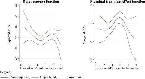
To further analyse the relationship between AIV commercialization and food security, we applied a continuous PSM model to the various food security indicators using the share of AIVs marketed as a treatment variable. We found that the total agricultural cropping output decreased significantly if the household sold only 20 to 40% of its AIV harvest, and the output stabilized around that level if the levels of commercialization increased (Figure 2).

Figure 2. Dose response and marginal treatment effect functions for the availability and access dimensions of food security. Source: Author

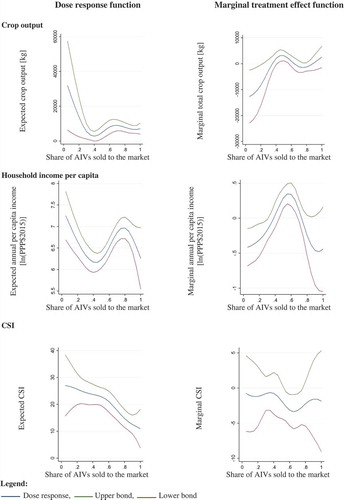
In contrast, the per capita household income showed a rather ambiguous relationship to different commercialization levels; while it first decreased with increasing commercialization levels, this trend turned at the point at which approximately 40% of the AIV harvest was sold. If households sold approximately 40 to 80% of their AIV harvest, this had a positive influence on their per capita income. This decline in income for the households that sold almost all their AIV harvest was no longer significant, as indicated by the large gap between the upper and lower bounds in the graph showing marginal treatment.

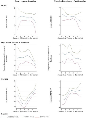
While the CSI significantly decreased linearly with increasing levels of AIV commercialization, indicating the stronger effect of the decision to sell AIVs on the access dimension of food security, more of the harvest was sold (Figure 3). The same was true for the stability dimension, as the MAHFP significantly increased with increasing shares of the AIV harvest sold.

The occurrence of diarrhoea decreased at higher levels of AIV commercialization, while the HDDS stayed the same. However, the rather large space between upper and lower bounds suggested an insignificant development, confirming the rather indistinct influence of AIV commercialization on the utilization dimension of food security in the binary case models (Tables 6,7). As the FCS did not show significant results in binary PSM and ESR, we do not discuss the continuous PSM results of this indicator here, but the results can be found in appendix A (Figure A2).

Figure 3. Dose response and marginal treatment effect functions for the availability and access dimensions of food security.

5. Discussion

In the results section, we reported factors that influence the farmers’ decisions to engage in commercial AIV production. Formal education, access to an extension service, participation in producer groups and an extensive social network positively influenced commercial AIV production. Thus, the same mechanism we found for the adoption of other agricultural innovations such as certifications or superior production standards seemed to apply to AIVs (Asfaw et al., 2010; Ngokkuen & Grote, 2012; Omiti et al., 2009). Previous research on AIVs suggested that poorer and less educated households focused on AIV production (Weinberger & Pichop, 2009), but we saw the opposite trend in our results. This may be a sign of a change in the status of AIVs in Kenya; AIVs are no longer seen as “poor people’s food” but rather are seen as a profitable business alternative, as suggested by (Cernansky, 2015).

If a household had access to irrigation water, they were significantly more likely to focus on commercial AIV production. Access to water also had a positive influence on the decision of smallholders to market vegetables to the export market in Kenya (Muriithi, Braun, Matz, & Virchow, 2016). Our results confirmed this relationship for AIVs in the domestic market, highlighting the importance of irrigation for the economic success of these crops (Mwangi & Crewett, 2019).

Farmers engaging in commercial AIV production were significantly more likely to be located close to a large city, which was confirmed by earlier findings in the literature (Gotor & Irungu, 2010; Omiti et al., 2009; Weinberger & Pichop, 2009). The reasons for this lie in the perishable nature of the products. Leafy vegetables such as AIVs need to be sold on the day of harvest, making the marketable range very limited if cooled storage is not available.

Regarding the impact of the decision to market AIVs, we find that farmers who sold AIVs had a higher per capita income than those who did not, which was consistent with recent findings emphasizing the income potential of AIVs for small-scale farmers and the capacity of AIVs to lift poor households out of poverty (Cernansky, 2015; Gotor & Irungu, 2010). Earlier findings mainly suggested a positive income effect of participation in the high value export market for horticultural crops (Muriithi & Matz, 2015), but our results showed that the Kenyan domestic market can in fact be an interesting target for smallholder farmers, at least in the case of AIVs.

However, the rate of specialization in commercial AIV production also played a very important role. The results of continuous PSM showed that the income effect was significantly negative if only a small share of the AIV harvest was sold to the market but positive when higher shares of the yield were marketed. The selling of a small percentage of the AIVs indicated that the households may have only sold the surplus beyond what was needed for their subsistence. This surplus usually occurs in the rainy season, when AIVs are available in abundance and prices are very low. An oversupply in the domestic vegetable market can further increase post-harvest losses (Muriithi et al., 2016). Thus, selling AIVs at this time can actually have a negative effect on the household income.

The food security status of the household was significantly enhanced in terms of the access and stability dimensions, as indicated by the positive influence of commercial AIV production on the CSI and the MAHFP indicator in both the binary and the continuous treatment cases. This confirmed our hypothesis that commercial AIV production increases food security and stability over time. According to our conceptual framework, this food security effect can derive from the following two pathways (Hartje et al., 2018): through either a change in crop portfolio leading to the increased and extended availability of AIVs that the household eats themselves or the positive income effects of focusing on AIVs as a cash crop that we saw in our models. The food security effect via the income pathway can also directly increase the stability of food security because AIVs are fast-growing crops that can generate profits within one to two months.

The HDDS and the occurrence of diarrhoea—indicators of the utilization dimension of food security—were positively influenced by AIV commercialization but not significant throughout all models. One reason for this could be the influence of other factors on those variables. The occurrence of diarrhoea and digestion problems can also be influenced by the sanitation system used or the hygienic practices established at home. Dietary diversity and food security in the household can also be influenced by nutrition education (Ilett & Freeman, 2004). While we controlled for the overall educational status of the household members, we do not have information on nutrition education that the households might have received. Another reason could be that the effects of commercial AIV production on food security mainly occur due to higher available income rather than through higher dietary diversity through the direct consumption of AIVs.

6. Conclusions

This article aimed to analyse the determinants of adopting commercial AIV production and the influence of adopting these crops as cash crops on household income and food security.

Our findings on the adoption determinants suggested that AIVs have indeed made the transition from “poor people’s food” to an interesting cash crop in Kenya. This was also supported by our econometric results suggesting that farmers who sell AIVs have a higher per capita income than those who do not and that this effect increased with increasing commercialization levels. The food security status of the household was significantly enhanced in the access and stability dimensions mainly due to an increase in available income than through a higher dietary diversity because farmers consumed the AIVs produced themselves.

Our results indicated that the geographic range of marketing is still limited for the majority of farmers who focus on these perishable crops, because the distance to urban markets still played a major role in the decision to adopt commercial AIV production. Since the distances from the production sites to urban markets in our study were all within half a day to a day of travel, we argue that post-harvest handling, such as adequate cooled storage, is still a major hindrance to farmers from rural areas.

A major limitation of observational studies is the self-selection bias of the treatment variable. We accounted for this with two different models, ESR and PSM, carefully discussed the underlying assumptions and variable choices and tested the robustness of the results. ESR has the advantage over PSM in handling unobserved heterogeneity. The significance of the results obtained with both approaches suggested an important relationship between AIV commercialization, household income and food security. Further, we have to keep in mind that the data has been collected in 2015, giving merely a snapshot of the situation at that time. Though to our knowledge, no significant policy measures regarding AIVs have been implemented in Kenya since 2015. Due to their richness in micronutrients, the main potential for AIVs in terms of food security is to fight hidden hunger. Anthropometric indicators that directly reveal hidden hunger in households, e.g., stunting rates among children, might give a clearer picture of this issue. Thus, to further support our findings on enhanced food security among commercial AIV producers, more extensive research with anthropometric measures should be considered in the future.

Acknowledgements

This publication is a product of the HORTINLEA project (http://www.hortinlea.org/) funded by the German Federal Ministry of Education and Research (BMBF) and co-financed by the German Federal Ministry of Economic Cooperation and Development (BMZ). The views expressed are purely those of the authors and may not under any circumstances be regarded as stating an official position of the BMBF and BMZ. The article processing charge (APC) was funded by the Open Access fund of Leibniz Universität Hannover.

Additional information

Funding

The authors received no direct funding for this research.

Notes on contributors

Henning Krause

Henning Krause is researcher and lecturer at Leibniz University Hannover. His research focuses on value chain development for fresh horticultural products in South East Asia and East Africa, as well as food security and income effects of horticultural production.

Anja Faße

Prof. Dr. Anja Faße is Chair of Environmental Policy and Resource Economics at the TUM Campus Straubing for Biotechnology and Sustainability (TUMCS). Her research foci are agroforestry, rural agricultural value chains, sustainability, poverty and food security in sub-Saharan Africa.

Ulrike Grote

Prof. Dr. Ulrike Grote is Director of the Institute for Environmental Economics and World Trade at Leibniz University Hannover. Research foci are environmental and development economics, with focus on South-East Asia and Africa; certification and trade; migration and agricultural policy.

Notes

1. HORTINLEA (Horticultural Innovation and Learning for Improved Nutrition and Livelihood in East Africa) is an interdisciplinary research project addressing food security in East Africa, particularly in Kenya, that focuses on AIV production, marketing and consumption.

Appendix A:

Additional Results

This appendix presents additional descriptive and econometric results mentioned in the paper.

Table A1. Description and descriptive statistics for explanatory variables used in the regressions

Livelihood dimensions	Variables	Description	Did not sell AIVs	Sold AIVs	Total
Human capital	Age of HH head	Age of household head [years]	52.58	51.12	51.57
			(12.93)	(12.45)	(12.61)
	Gender of HH head	[1 = male, 0 = female]	0.820	0.814	0.816
			(0.385)	(0.39)	(0.388)
	Higher education	Number of HH members with higher education	0.590	0.534	0.551
			(0.959)	(0.979)	(0.972)
Physical/natural capital	Total land	Total land holdings owned by the household [ha]	0.814	0.845	0.836
			(1.133)	(1.184)	(1.168)
	Asset score	Household’s asset score	3,247	3,091	3,139
			(4,581)	(4,581)	(4,581)
Social capital	Producer group	Household is member of a producer group [1 = yes, 0 = no]	0.263	0.423***	0.374
			(0.441)	(0.495)	(0.484)
	Information extension service	HH has access to market information from agriculture extension service [1 = yes, 0 = no]	0.387	0.532***	0.487
			(0.488)	(0.5)	(0.5)
	People known	Number of people the HH knows in the village	119.666	148.292	139.493
			(135.942)	(150.62)	(146.766)
Source of finance	Share of crop production	Share of income from agriculture in total household income	0.279	0.330	0.314
			(0.289)	(0.281)	(0.284)
	Savings	Total amount of savings of the household [PPP$(2015)]	1,772	1,703	1,724
			(4,203)	(4,064)	(4,104)
Public infrastructure	Distance to next city	Distance to Kisumu and Nairobi [km]	86.50	68.06	73.72
			(40.81)	(38.88)	(40.36)
	Distance to tarmacked road	Distance to next tarmacked road [km]	3.87	3.46	3.59
			(6.34)	(5.19)	(5.57)
	Distance to AgroVet	Distance to next agricultural input shop service [km]	2.76	3.23	3.09
			(2.94)	(3.99)	(3.7)
	Access to irrigation water	Household had access to irrigation water [1 = yes, 0 = no]	0.157	0.294***	0.252
			(0.364)	(0.456)	(0.435)
Shocks	Shock	Household experienced a shock in income or assets in the last year [1 = yes, 0 = no]	0.945	0.953	0.950
			(0.229)	(0.212)	(0.217)

HH = household, Standard errors in brackets, * = significantly different between sellers and non-sellers at the 10% level, ** = significant at the 5% level, *** = significant at the 1% level. Source: own data.

Table A2. Description and descriptive statistics for outcome variables used in the regressions

Food security dimensions	Variables	Description	Did not sell AIVs	Sold AIVs	Total
Availability	Crop_output	Total output of cropping activity [kg]	7,456	8,595	8,245
			(36,062)	(25,562)	(29,172)
Access	hhinc_pc	Annual HH income per capita [PPP$(2015)]	1,286	1,586***	1,494
			(1,681)	(2,024)	(1,929)
	FCS	Food consumption score	70.68	70.20	70.35
			(17.13)	(15.27)	(15.85)
	CSI	Coping strategy index	22.85	19.70	20.66
			(27.45)	(24.15)	(25.23)
Utilization	HDDS	Household Dietary Diversity Index	8.779	8.937	8.888
			(1.484)	(1.461)	(1.468)
	Days_missed	Total number of days HH members missed work/school because of stomach ache/diarrhoea	1.608	1.395	1.460
			(5.041)	(6.271)	(5.918)
Stability	MAHFP	Months of adequate household food Provisioning	8.793	9.681***	9.408
			(4.173)	(3.753)	(3.906)

HH = household, Standard errors in brackets, * = significantly different between sellers and non-sellers at the 10% level, ** = significant at the 5% level, *** = significant at the 1% level. Source: own data.

Figure A1. GPS points of the survey area (circles) and cities and towns (diamonds).  Source: own construction.

Figure A2. Dose response and marginal treatment effect functions for the food consumption score (FCS). Source: Own data.

Appendix B:

Robustness Checks Propensity Score Matching

In this appendix we summarize measures to ensure optimal bias reduction in Propensity Score Matching (PSM) and robustness checks applied to validate the findings.

In radius and kernel matching, certain adjustments on the algorithm influence its bias reduction property. For radius matching, it was found that optimal bias reduction was reached with a calliper equalling a fifth of the standard deviation of the propensity score (Austin, 2011). Following this argument, we set our caliper to 0.065. The bandwidth in kernel matching needs to be balanced carefully on a case-to-case basis to ensure optimal bias reduction without an excessive increase in variance of the estimates (Caliendo & Kopeinig, 2008). We found a bandwidth of 0.1 to be optimal for our case.

To reduce the problem of variance overestimation in the ATT (Heckman, Ichimura, & Todd, 1998), we used bootstrapped standard errors with 500 repetitions, which is considered high enough for the reduction effect and still practicable for computational capacities (Lechner, 2002).

According to Rosenbaum & Rubin, 1983b), the ATT is only defined in the region of common support. For this, all households with the same explanatory variable $X$ need to have a positive probability of selling AIVs or choosing not to sell AIVs. Fourteen observations did not fulfil the common support condition throughout the three algorithms and were removed from the analysis. Figure B1 shows the distribution of the propensity scores, and Table B1 shows the number of observations that were dropped to comply with the common support condition.

Table B1. Binary PSM: Imposition of common support

Sample	Off support	On support	Total
Untreated	2	215	217
Treated	12	477	489
Total	14	692	706

Source: own data.

We used standardized bias tests, t-tests and F-tests to evaluate the quality of the matching that are summarized in Tables B2,B3. A mean bias of approximately 5% after matching has been established as a level of bias reduction for a good match in PSM (Caliendo & Kopeinig, 2008). A much lower level than this is reached in calliper and kernel matching. Nearest neighbour matching has a slightly higher remaining bias. However, individual t-tests and the overall F-test were insignificant in all matching algorithms, indicating that the matching of the explanatory variable $X$ was a success. To control for hidden bias, we applied the Rosenbaum bounds approach (Rosenbaum, 2002), but only for statistically significant results (Hujer, Caliendo, & Thomsen, 2004).

Figure B1. Distribution of the propensity scores.  Source: own data.

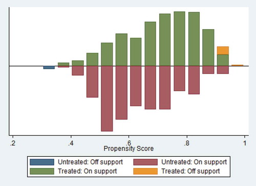
Table B2. Binary PSM: Overall bias reduction and F-test after matching

Sample	Pseudo-R2	LR chi2	p> chi2	MeanBias	MedBias
Unmatched	0.071	62.03	0	13.8	5.8
NNM	0.015	19.68	0.103	6.3	5.1
RM	0.005	6.42	0.929	4.3	4.9
KM	0.005	7.04	0.9	4.4	4.6

NNM = Nearest neighbour matching, RM = Radius matching, KM = Kernel matching. Source: own data.

Table B3. Binary PSM: Bias reduction and level of significance of explanatory variables after matching

Matching algorithm	Unmatched		Nearest neighbour matching			Radius matching			Kernel matching
Variable	%bias	p>|t|	%bias	% bias eduction	p>|t|	%bias	% bias reduction	p>|t|	%bias	% bias reduction	p>|t|
Age of HH head	−11.5	0.158	−14.3	−25.2	0.022	−3.7	67.6	0.566	−4	65	0.536
Gender of HH head	−1.6	0.841	−3.8	−130.4	0.553	0.2	86.4	0.973	−0.1	96.6	0.993
Higher education	−5.8	0.480	2.6	55.2	0.673	4.6	20.1	0.443	4	30.1	0.504
Total land	2.7	0.745	−1.3	51	0.841	0.7	72.9	0.912	1.1	57.9	0.863
Asset score	−3.6	0.650	7.3	−101.1	0.191	0.6	82.2	0.916	0.8	79	0.9
Producer group	34.3	0.000	−8.1	76.5	0.239	−6.4	81.2	0.347	−6.1	82.1	0.371
People known	20	0.017	15	24.7	0.025	8.4	57.7	0.222	9.5	52.6	0.167
Share of crop production	17.8	0.028	−3.8	78.7	0.581	−2.1	88	0.754	−1.4	92	0.833
Total savings	−1.7	0.837	−0.3	81.8	0.96	6.4	−280.1	0.272	6.3	−276.7	0.275
Distance to next city	−41.7	0.000	−0.5	98.8	0.939	−4.9	88.4	0.464	−5.6	86.6	0.401
Distance to tarmacked road	1.2	0.882	10.4	−775.2	0.104	5.9	−393.1	0.363	5.7	−378.4	0.378
Access to irrigation water	33.4	0.000	−5.1	84.8	0.475	6.7	80	0.333	8.1	75.7	0.238
Shock	3.7	0.641	−9.5	−153.7	0.089	−4.9	−30.1	0.413	−4.6	−24.1	0.436

HH = household. Source: own data.

Appendix C:

Instrument and Further Results Endogenous Switching Regression

In this section we elaborate on the choice of the instrument used for the Endogenous Switching Regression (ESR) and show the extended model output for each outcome variable.

To account for self-selection bias in the outcome equation, we included a selection instrument and the inverse Mills ratio of the selection equation (Shiferaw et al., 2014b). As selection instruments, we used the distance of the household’s main residence to the nearest AgroVet market and a dummy variable of one if the household has access to information on market prices and agricultural production from agricultural extension officers. AgroVet markets are specialized shops in Kenya where households can buy supplies needed for their farming activities (seeds, fertilizers, pesticides, animal feeds, etc. but also obtain information on input use and market developments. Agricultural extension officers can provide very useful information for households who want to intensify their production and commercialize a specific crop. Those factors can thus facilitate the process of adopting commercializing activities but can have little impact on income or food security, as the factors still have to be put to use by the household. Access to input markets and to reliable sources of information are well-established instruments to promote the adoption of agricultural technologies or commercializing agricultural crops (Fischer & Qaim, 2014; Shiferaw et al., 2014b). To test for the statistical validity of the instrument, we used the falsification test of Di Falco et al. (2011b), which shows that the vector of the instruments has an influence on the adoption decision but not on the outcome variables (Table C1).

Table C1. ESR: Influence of instrument on treatment and outcome variable

Treatment	Chi^2	Prob. >chi^2
sell_topAIVs	9.59	0.0083
Outcome variables
Crop output	1.83	0.1611
HHInc per capita	1.9	0.1503
CSI	0.92	0.399
HDDS	1.38	0.2528
Days missed because of diarrhoea	0.69	0.5022
MAHFP	0.06	0.9377

Source: own data.

References

- Abukutsa-Onyango, M. O., [M.O]. (2010). African indigenous vegetables in Kenya. Strategic repositioning in the horticultural sector. Nairobi, Kenya: Jomo Kenyatta University of Agriculture and Technology.
- Asfaw, S., Mithöfer, D., & Waibel, H. (2010). What impact are EU supermarket standards having on developing countries’ export of high-value horticultural products? Evidence from Kenya. Journal of International Food & Agribusiness Marketing, 22(3–4), 252–33. doi:10.1080/08974431003641398
- Asfaw, S., Shiferaw, B., Simtowe, F., & Lipper, L. (2012). Impact of modern agricultural technologies on smallholder welfare: Evidence from Tanzania and Ethiopia. Food Policy, 37(3), 283–295. doi:10.1016/j.foodpol.2012.02.013
- Ayodele, V. I., Makaleka, M. B., Chaminuka, P., & Nchabeleng, L. M. (2011). Potential role of indigenous vegetable production in household food security: A case study in the Limpopo Province of South Africa. Acta Horticulturae. (911), 447–453. doi:10.17660/ActaHortic.2011.911.52
- Bernard, T., Taffesse, A. S., & Gabre-Madhin, E. (2008). Impact of cooperatives on smallholders’ commercialization behavior: Evidence from Ethiopia. Agricultural Economics, 39(2), 147–161. doi:10.1111/j.1574-0862.2008.00324.x
- Bilinsky, P., & Swindale, A. (2010). Months of adequate household food provisioning (MAHFP) for measurement of household food access: Indicator guide - version 4. Washington D.C., USA: Food and Nutrition Technical Assistance.
- Caliendo, M., & Kopeinig, S. (2008). Some practical guidance for the implementation of propensity score matching. Journal of Economic Surveys, 22(1), 31–72. doi:10.1111/j.1467-6419.2007.00527.x
- Cernansky, R. (2015). The rise of Africa’s super vegetables. Nature, 522(7555), 146–148. doi:10.1038/522146a
- Coates, J. (2013). Build it back better: Deconstructing food security for improved measurement and action. Global Food Security, 2(3), 188–194. doi:10.1016/j.gfs.2013.05.002
- Croft, M. M., Marshall, M. I., & Weller, S. C. (2014). Consumers’ preference for quality in three African indigenous vegetables in Western Kenya. Journal of Agricultural Economics and Development, 3(5), 67–77.
- DFID. (1999). Sustainable livelihoods guidance sheets. London, United Kingdom: Derpartment for International Development.
- Di Falco, S., Veronesi, M., & Yesuf, M. (2011b). Does adaptation to climate change provide food security?: A micro-perspective from Ethiopia. American Journal of Agricultural Economics, 93(3), 829–846. doi:10.1093/ajae/aar006
- Ewbank, R., Nyang, M., Webo, C., & Roothaert, R. L. (2007). Socio-economic assessment of four MATF funded projects FARM-Africa Working Papers. London, United Kingdom. doi:10.1094/PDIS-91-4-0467B
- Faber, M., van Jaarsveld, P. J., & Laubscher, R. (2009). The contribution of dark-green leafy vegetables to total micronutrient intake of two- to five-year-old children in a rural setting. Water SA, 33(3). doi:10.4314/wsa.v33i3.49153
- FAO. (2008). An introduction to the basic concepts of food security. Rome, Italy: Author. doi:10.18356/151a3bf9-en
- FAO, IFAD, & WFP. (2013). The state of food insecurity in the world 2013: The multiple dimensions of food security. Rome, Italy: Food and Agriculture Organization of the United Nations (FAO).
- Fereres, E., Goldhamer, D. A., & Parsons, L. R. (2003). Irrigation water management of horticultural crops. HortScience, 38(5), 1036–1042. doi:10.21273/HORTSCI.38.5.1036
- Gido, E. O., Ayuya, O. I., Owuor, G., Bokelmann, W., & Yildiz, F. (2016). Consumers choice of retail outlets for African indigenous vegetables: Empirical evidence among rural and urban households in Kenya. Cogent Food & Agriculture, 2(1), 1442. doi:10.1080/23311932.2016.1248523
- Gockowski, J., Mbazo’o, J., Mbah, G., & Fouda Moulende, T. (2003). African traditional leafy vegetables and the urban and peri-urban poor. Food Policy, 28(3), 221–235. doi:10.1016/S0306-9192(03)00029-0
- Gotor, E., & Irungu, C., [Charity] (2010). The impact of bioversity international’s African leafy vegetables programme in Kenya. Impact Assessment and Project Appraisal, 28(1), 41–55. doi:10.3152/146155110X488817
- Habwe, F. O., Walingo, M. K., Abukutsa-Onyango, M. O., [Mary], & Oluoch, M. O. (2009). Iron content of the formulated East African indigenous vegetable recipes. African Journal of Food Science, 3(12), 393–397.
- Hartje, R., Bühler, D., & Grote, U. (2018). Eat your fish and sell it, too – livelihood choices of small-scale fishers in Rural Cambodia. Ecological Economics, 154, 88–98. doi:10.1016/j.ecolecon.2018.07.002
- Hatløy, A., Hallund, J., Diarra, M. M., & Oshaug, A. (2000). Food variety, socioeconomic status and nutritional status in urban and rural areas in Koutiala (Mali). Public Health Nutrition, 3(1), 57. doi:10.1017/S1368980000000628
- Headey, D., & Ecker, O. (2013). Rethinking the measurement of food security: From first principles to best practice. Food Security, 5(3), 327–343. doi:10.1007/s12571-013-0253-0
- Hirano, K., & Imbens, G. W. (2005). The propensity score with continuous treatments. In A. Gelman & X.-L. Meng (Eds.), Wiley series in probability and statistics. Applied Bayesian modeling and causal inference from incomplete-data perspectives: An essential journey with Donald Rubin’s statistical family (pp. 73–84). Chichester: Wiley.
- Ilett, S., & Freeman, A. (2004). Improving the diet of toddlers of Pakistani origin: A study of intensive dietary health education. The Journal of Family Health Care, 14(1), 16–19.
- Irungu, C., Mburu, J., Maundu, P., Grum, M., & Hoeschle-Zeledon, I. (2007). Analysis of markets for African leafy vegetables within Nairobi ant its environs and implications for on-farm conservation of biodiversity. Rome, Italy: Global Facilitation Unit for Underutilized Species (GFU).
- Jena, P. R., Chichaibelu, B. B., Stellmacher, T., & Grote, U. (2012). The impact of coffee certification on small-scale producers’ livelihoods: A case study from the Jimma Zone, Ethiopia. Agricultural Economics, 43(4), 429–440. doi:10.1111/j.1574-0862.2012.00594.x
- Kamga, R. T., Kouamé, C., Atangana, A. R., Chagomoka, T., & Ndango, R. (2013). Nutritional evaluation of five African Indigenous vegetables. Journal of Horticultural Research, 21(1), 99–106. doi:10.2478/johr-2013-0014
- Kassie, M., Jaleta, M., & Mattei, A. (2014). Evaluating the impact of improved maize varieties on food security in Rural Tanzania: Evidence from a continuous treatment approach. Food Security, 6(2), 217–230. doi:10.1007/s12571-014-0332-x
- KNBS. (2015). Economic survey 2015. Nairobi, Kenya: Kenyan National Bureau of Statistics.
- Kuşçu, H., Çetin, B., & Turhan, A. (2009). Yield and economic return of drip‐irrigated vegetable production in Turkey. New Zealand Journal of Crop and Horticultural Science, 37(1), 51–59. doi:10.1080/01140670909510249
- Legwaila, G. M., Mojeremane, W., Madisa, M. E., Mmolotsi, R. M., & Rampart, M. (2011). Potential of traditional food plants in rural household food security in Botswana. Journal of Horticulture and Forestry, 3(6), 171–177.
- Liao, T. F. (2005). Assessing hidden bias in the estimation of causal effect in longitudinal data by using a matching estimator with rosenbaum bounds. Illimois, USA: University of Illinois.
- Lovon, M., & Mathiassen, A. (2014). Are the world food programme’s food consumption groups a good proxy for energy deficiency? Food Security, 6(4), 461–470. doi:10.1007/s12571-014-0367-z
- Maxwell, D., & Caldwell, R. (2008). The coping strategies index - field methods manual, second edition. Geneva, Switzerland: Cooperative for Assistance and Relief Everywhere (CARE).
- Mbhenyane, X., Venter, C., Vorster, H., & Steyn, S. (2016). Nutrient intake and consumption of indigenous foods among college students in Limpopo Province. South African Journal of Clinical Nutrition, 18(1), 32–38. doi:10.1080/16070658.2005.11734035
- Mbugua, G. W., [G. W.], Gitonga, L., Ndungu, B., Gatambia, E., Manyeki, L., & Karoga, J. (2011). African indigenous vegetables and farmer-preferences in Central Kenya. Acta Horticulturae. (911), 479–485. doi:10.17660/ActaHortic.2011.911.56
- Modi, M., Modi, A., & Hendriks, S. (2006). Potential role for wild vegetables in household food security: A preliminary case study in Kwazulu-Natal, South Africa. African Journal of Food, Agriculture, Nutrition and Development, 6(1). doi:10.4314/ajfand.v6i1.19167
- Msuya, J. M., Mamiro, P., & Weinberger, K. (2009). Iron, zinc and ß-Carotene nutrient potential of non-cultivated indigenous vegetables in Tanzania. Acta Horticulturae. (806), 217–222. doi:10.17660/ActaHortic.2009.806.26
- Muriithi, B. W., Braun, J. V., Matz, J. A., & Virchow, D. (2016). The dynamics of smallholders’ participation in the commercialization of high-value horticultural crops: A case of vegetable producers in Kenya. Acta Horticulturae. (1128), 263–270. doi:10.17660/ActaHortic.2016.1128.40
- Muriithi, B. W., & Matz, J. A., [Julia] (2015). Welfare effects of vegetable commercialization: Evidence from smallholder producers in Kenya. Food Policy, 50, 80–91. doi:10.1016/j.foodpol.2014.11.001
- Muthayya, S., Rah, J. H., Sugimoto, J. D., Roos, F. F., Kraemer, K., Black, R. E., & Noor, A. M. (2013). The global hidden hunger indices and maps: An advocacy tool for action. PLoS ONE, 8(6), e67860. doi:10.1371/journal.pone.0067860
- Mwangi, J. K., & Crewett, W. (2019). The impact of irrigation on small-scale African indigenous vegetable growers’ market access in peri-urban Kenya. Agricultural Water Management, 212, 295–305. doi:10.1016/j.agwat.2018.06.036
- Mwaura, S. N., Muluvi, A. S., & Mathenge, M. K. (2013, September 22-25). African leafy vegetables and household wellbeing in Kenya: A disaggregation by gender. Hammamet, Tunisia: 4th International Conference of the African Association of Agricultural Economists.
- Ndenga, E. A., Achigan-Dako, E. G., Mbugua, G., Maye, D., & Ojanji, W. (2013). Agricultural diversification with indigenous vegetables for cash cropping and Nutrition: examples from Rift Valley and Central Provinces in Kenya. Acta Horticulturae. (979), 549–558. doi:10.17660/ActaHortic.2013.979.59
- Ngokkuen, C., & Grote, U. (2012). Geographical indication for jasmine rice: Applying a logit model to predict adoption behavior of Thai farm households. Quarterly Journal of International Agriculture. (892–2016–65165), 29. Retrieved from http://ageconsearch.umn.edu/record/155476
- Omiti, J. M., Otieno, D. J., Nyanamba, T. O., & McCullough, E. B. (2009). Factors influencing the intensity of market participation by smallholder farmers: A case study of rural and peri-urban areas of Kenya. African Journal of Agricultural and Resource Economics, 3(1), 1–26. Retrieved from https://ideas.repec.org/a/ags/afjare/56958.html
- Oster, E. (2017). Unobservable selection and coefficient stability: Theory and evidence. Journal of Business & Economic Statistics, 40, 1–18. doi:10.1080/07350015.2016.1227711
- Rapsomanikis, G. (2015). The economic lives of smallholder farmers - An analysis based on household data from nine countries. Rome: Food and Agriculture Organization of the United Nations.
- Rogers, E. M. (2003). Diffusion of innovations (Fifth edition, Free Press trade paperback edition). Social science. New York, London, Toronto, Sydney: Free Press. Retrieved from http://www.loc.gov/catdir/bios/simon052/2003049022.html
- Rosenbaum, P. R., & Rubin, D. B. (1983b). The central role of the propensity score in observational studies for causal effects. Biometrika, 70(1), 41–55. doi:10.1093/biomet/70.1.41
- Scoones, I. (1998). Sustainable rural livelihoods: A framework for analysis. IDS Working Papers. p. 72.
- Shiferaw, B., Kassie, M., Jaleta, M., & Yirga, C. (2014b). Adoption of improved wheat varieties and impacts on household food security in Ethiopia. Food Policy, 44, 272–284. doi:10.1016/j.foodpol.2013.09.012
- Sibhatu, K. T., Krishna, V. V., & Qaim, M. (2015). Production diversity and dietary diversity in smallholder farm households. Proceedings of the National Academy of Sciences of the United States of America, 112(34), 10657–10662. doi:10.1073/pnas.1510982112
- Singh, I., Squire, L., & Strauss, J. (1986). Agricultural household models: Extensions, applications, and policy. Baltimore, MD, USA: The Johns HopkinsUniversity Press.
- Singh, S., Singh, D. R., Singh, L. B., Chand, S., & Roy, S. D. (2013). Indigenous vegetables for food and nutritional security in Andaman and Nicobar Islands, India. International Journal of Agriculture and Food Science Technology, 4(5), 503–512.
- Swindale, A., & Bilinsky, P. (2006). Household dietary diversity score (HDDS) for measurement of household food access: Indicator guide - version 2. Washington D.C., USA: Food and Nutrition Technical Assistance.
- Weinberger, K., [Katinka], & Msuya, J., [John]. (2004). Indigenous vegetables in Tanzania: Significance and prospects. Technical bulletin/Asian vegetable research and development center: Vol. 31. Shanhua: AVRDC.
- Weinberger, K., [Katinka], Pasquini, M., Kasambula, P., & Abukutsa-Onyango, M. O. (2011). Supply chains for indigenous vegetables in urban and peri-urban areas of uganda and kenya: A gendered perspective. In D. Mithöfer & H. Waibel (Eds.), Vegetable production and marketing in Africa: Socio-economic research (pp. 169–182). Wallingford: CABI.
- Weinberger, K., [Katinka], & Pichop, G. N. (2009). Marketing of African indigenous vegetables along urban and peri-urban supply chains in Sub-Saharan Africa. In C. M. Shackleton, M. Pasquini, & A. W. Drescher (Eds.), African indigenous vegetables in urban agriculture (pp. 225–244). London, Sterling, VA: Earthscan.
- WFP. (2008). Food consumption analysis – calculation and use of the food consumption score in food security analysis. Rome, Italy: United Nations World Food Programme.
- WFP. (2015). Kenya food security and outcome Monitoring: consolidated report. World Food Programme website. Retrieved from https://www.wfp.org/content/kenya-food-security-and-outcome-monitoring-2015
- WFP. (2018). World food programme country report: Kenya. World Food Programme website. Retrieved from http://www1.wfp.org/countries/kenya
References Appendices
- Austin, P. C. (2011). Optimal caliper widths for propensity-score matching when estimating differences in means and differences in proportions in observational studies. Pharmaceutical Statistics, 10(2), 150–161. doi:10.1002/pst.433
- Di Falco, S., Veronesi, M., & Yesuf, M. (2011a). Does adaptation to climate change provide food security?: A micro-perspective from Ethiopia. American Journal of Agricultural Economics, 93(3), 829–846. doi:10.1093/ajae/aar006
- Fischer, E., & Qaim, M. (2014). Smallholder farmers and collective action: What determines the intensity of participation? Journal of Agricultural Economics, 65(3), 683–702. doi:10.1111/1477-9552.12060
- Heckman, J. J., Ichimura, H., & Todd, P. (1998). Matching as an econometric evaluation estimator. Review of Economic Studies, 65(2), 261–294. doi:10.1111/1467-937X.00044
- Hujer, R., Caliendo, M., & Thomsen, S. L. (2004). New evidence on the effects of job creation schemes in Germany—a matching approach with threefold heterogeneity. Research in Economics, 58(4), 257–302. doi:10.1016/j.rie.2004.07.001
- Lechner, M. (2002). Some practical issues in the evaluation of heterogeneous labour market programmes by matching methods. Journal of the Royal Statistical Society: Series A (Statistics in Society), 165(1), 59–82. doi:10.1111/1467-985X.0asp2
- Rosenbaum, P. R. (2002). Observational studies (2nd). Springer series in statistics. New York, NY: Springer New York. doi:10.1007/978-1-4757-3692-2
- Rosenbaum, P. R., & Rubin, D. B. (1983a). The central role of the propensity score in observational studies for causal effects. Biometrika, 70(1), 41–55. doi:10.1093/biomet/70.1.41
- Shiferaw, B., Kassie, M., Jaleta, M., & Yirga, C. (2014a). Adoption of improved wheat varieties and impacts on household food security in Ethiopia. Food Policy, 44, 272–284. doi:10.1016/j.foodpol.2013.09.012