Performance evaluation and yield stability of upland rice (Oryza sativa L.) varieties in Ethiopia

Abstract

Multi-environment evaluation of genotypes is important to identify the response of genotypes across environments and helps to know which genotypes would be appropriate in which production areas. Thirteen upland rice genotypes were evaluated in a randomized complete block design at Tepi, Assosa, Bako, and Bonga research centers in 2017, 2018, and 2019 cropping season with the objective of examining the agronomic performance and evaluating the yield stability of the varieties. The combined analysis of variance for yield and other agronomic characteristics revealed that main effects, genotypes, locations, years, and the three-way (G X L X Y) interaction effects revealed a significant difference for the measured traits. Moreover, AMMI analysis of variance also showed a highly significant difference for genotypes, environment, and genotype x environment (GE) interaction for grain yield. Environment effect (61.64%) was responsible for the greatest part of the variation, followed by genotype by environment interaction (20.86%) and genotype (6.97%) effects. The AMMI analysis explained 69.17% of the GxE variance, while GGE captured 72.76% of the GGE variance. Based on the GGE, AMMI analysis genotype variety Hidassie (G4), 4238.7 Kg ha⁻¹ followed by NERICA-4 (G3), 4183.5 Kg ha⁻¹ were the most stable and high yielding genotypes and recommended for production for the testing sites and similar upland rice-producing areas of Ethiopia.

Key words:

• Adaptation
• GxE
• rice
• stability
• upland ecosystem

PUBLIC INTEREST STATEMENT

Rice is one of the recently introduced cereal crops in Ethiopia. Even though it is a recent introduction, the crop is getting wider acceptance in many regions of the country. The presence of huge potential in the country, good varieties for the different ecosystems, and easy use of the crop for food preparations makes its expansion to go faster. In rice-producing areas, not only the grains but also the straw is used for cattle feed. Rice growers in many areas of Ethiopia prefer the variety that has good yield, resistant to insect pests, early maturing, and variety that has white caryopsis color. So, an adaptation trial was conducted across locations and years to identify and recommend the better yielding and stable genotypes and also meet the producers’ interest for the upland rice-producing areas of Ethiopia.

Competing interests

The authors declare no competing interests.

1. Introduction

Rice (Oryza sativa L.) is most commonly produced in Asia, Africa, and Australia (Dogara & Jumare, 2014). It is the third most cultivated cereal crop in the world, after wheat and maize (FAO, 2014). It is the most common staple food for more than half of the world’s population and provides up to 50% of the dietary caloric supply and a substantial part of the protein intake in Asia (Muthayya et al., 2014).

Rice is a recently introduced crop in Ethiopia after the wild rice (O. longistaminata) was observed in the swampy and waterlogged areas of Fogera and Gambella plains (Gebey et al., 2012). Even though it is recently introduced, the government of Ethiopia has given due emphasis as a millennium crop for assuring food security and as an income source (Astewl, 2010). After its introduction, the production and productivity of the commodity are increasing from year to year. Currently, rice is produced in Amhara, Southern Nations, Nationalities and Peoples (SNNPR), Oromiya, Somali, Gambella, Benishangul Gumuz, and Tigray regions (CSA (Central Statistical Agency), 2011; Gebey et al., 2012; MoARD, 2010).

Even though both production and productivity have been increasing from year to year, the national average productivity is low as compared to other rice-producing countries. This could be due to lack of adapted and high yielding varieties, lack of extension services to the new technologies, terminal drought, diseases like sheath rot and rice blast, termite attack, cold problem, and lack of awareness about the technologies and its packages (Abebaw, 2018).

The response of the crops to varying environments will depend on the phenology, crop variety, and growth stage of the crop species. Different responses of genotypes across environments are the main challenge facing plant breeders. This is termed as genotype–environment interaction (Comestock & Moll, 1963). Significant G × E interaction indicates that all phenotypic responses of genotypes to varying agro-ecological conditions are not consistent. These would be due to rank change of the genotypes from location-to-location and/or from year-to-year. GxE interactions have greater importance in plant breeding as they reduce the stability of genotypic values under diverse environments. Therefore, the present investigation was planned to evaluate the agronomic performance and assessing the stability of different upland rice varieties using AMMI and GGE biplot analyses.

2. Material and methods

A field experiment was conducted at Assosa, Tepi, Bako, and Bonga Agricultural Research Centers in 2017, 2018, and 2019 cropping seasons in the rain-fed upland condition. The locations are potential rice-growing areas situated in the Southwest part of Ethiopia. In 2017, the trial was conducted at Assosa and Tepi, in 2018 at Bako and Bonga, and in 2019 at Assosa and Tepi. The descriptions of the trail sites are indicated in Table 1. Thirteen upland rice varieties released by national and regional research centers in Ethiopia were evaluated in a randomized complete block design replicated three times, on a plot size of 5 m long × 1.5 m width. A spacing of 0.25, 0.5, and 1.5 m were used between rows, plots, and blocks, respectively. A seed rate of 60 kg ha⁻¹ was used. Fertilizer application and weeding were carried out following the local recommendations.

Table 1. Description of experimental locations

Location	Elevation (m)	Latitude	Longi tude	Annual rain fall (mm)	Mean temperature (^o C)		Soil type
					Min	Max
Assosa	1668	9°45ʹN	34°44ʹE	1100	10.0	26.9	Vertisols
Tepi	1200	7°3 ’N	35°18ʹE	1522	15.0	30.0	Nitisols
Bako	1650	9° 6ʹN	37° 9ʹE	1431	13.3	28.0	Sandy-clay
Bonga	1700	7° 0ʹN	35° 55ʹE	1801	13.3	28.0	Vertisols

Data were recorded on five randomly selected plants from the middle four rows for panicle length, plant height, number of filled-grains per panicle while the number of days to heading and number of days for maturity were recorded on a plot basis. Grain yield and thousand seed weight were taken on a plot basis from four harvestable rows. Fertilizer application and weeding were carried out following the local recommendations. The combined data across locations and years were used to compute analysis of variance (ANOVA) using GenStat version 12 edition software package (Payne et al., 2009).

The responses of the genotypes were evaluated using Additive Main-effect and Multiplicative Interaction (AMMI), Genotype and Genotype-Environment interaction (GGE), stability measures for the same set of data. The GGE-biplot analysis was used for ranking genotypes based on grain yield performance and stability for detecting wider and/or specifically adapted genotype(s) (Yan, 2016). Additive Main-effect and Multiplicative Interaction (AMMI) was also computed as per Zobel et al. (1988):

${\mathrm{Y}}_{ijk}=\mu +{\mathrm{G}}_i+{\mathrm{E}}_J+\sum _{k=1}^m{\lambda }_{\mathrm{k}}{\alpha }_{\mathrm{i}\mathrm{k}}{\gamma }_{\mathrm{j}\mathrm{k}}+p_{\mathrm{i}\mathrm{j}}$

Where ${\mathrm{Y}}_{ijk}$= the yield of i^th genotype in the j^th environment, G_{i =} the mean of _the i^th genotype minus the grand mean, ${\mathrm{E}}_J$= the mean of the j^th environment minus the grand mean, ${\lambda }_{\mathrm{k}}$ = the square root of the eigenvalue of the k^th IPCA axis, ${\alpha }_{\mathrm{i}\mathrm{k}}$ and ${\gamma }_{\mathrm{j}\mathrm{k}}$ = the principal component scores for IPCA axis k of the i^th genotypes and the j^th environment, $p_{\mathrm{i}\mathrm{j}}$ = the deviation from the model.

3. Results and discussion

3.1. Analysis of variance for agronomic traits

The combined analysis of variance for yield and other agronomic characteristics is presented in Table 2. The result revealed that the main effects, genotype (G), location (L), and year (Y) showed a highly significant (P ≤ 0.001) difference for grain yield, and other agronomic traits. The L × Y had also showed a highly significant difference (P ≤ 0.001) for number of days to heading, number of days to maturity, panicle length, plant height, number of filled grains, thousand seed weight, and grain yield while the number of days to maturity and plant height were nonsignificant for in G × L and L × Y, respectively. This is in agreement with the findings of Sewagegne et al. (2013).

Table 2. Combined analysis of variance of 13 upland rice varieties evaluated in upland rice-producing areas of Ethiopia

Source of variations	Mean squares
	DH	DM	PL	PH	NFG	TSWT	GY
Replication	322.6***	257.2***	2.5 ns	225.1 ns	3277.7***	1.1 ns	1343909**
Genotype (G)	932.4***	168.9***	18.2***	692.8***	2111.7***	107.1***	3378154***
Loction (L)	3336.7***	3160.8***	42.1***	2520***	90928.0***	396.3***	21509591***
Year (Y)	851.1***	12.4**	15.0**	4889.1***	14393.6***	943.6***	165874708***
G x L	125.8***	28.6ns	5.8***	324.4**	865.0***	21.6***	2290418***
G x Y	53.2ns	12.9 ns	3.5ns	36.8ns	597.5 ns	15.7*	2037007***
L x Y	1132.8***	2323.2***	279.5***	275.1ns	68558.1***	834.4***	128287783***
G x L x Y	45.2	11.8 ns	2.4 ns	147.6 ns	407.9ns	14.2 ns	1209047***
Residual	47.3	24.1	3.1	168.90	370.0	9.0	380291
Total	158.7	79.4	5.7	258.69	2011.4	29.4	2497379.3

DH = number of days to 50% heading, DM =number of days to 85% maturity, PL =Panicle length, PH = Plant height, NFG =Number of filled grains, TSWT = Thousand seed weight, and GY = Grain yield (Kg ha⁻¹)

On the other hand, the three-way interaction of G × L × Y effects was highly significant (P ≤ 0.001) only for grain yield and nonsignificant for number of days to heading, number of days to maturity, panicle length, plant height, number of filled grains per panicle, and thousand seed weight. The nonsignificant response of genotypes across years and across locations and years indicated that the genotypes would respond in a similar manner while a significant (P ≤ 0.05) three-way interaction leads to further analysis to determine the magnitude of G×E and separate into component multiplicative terms, and to estimate yield stability of the genotypes.

The agronomic mean performance indicated in Table 3 showed that the genotypes gave comparable and good grain yield to their yield when they were released. The mean grain yield of the tested genotypes was ranged from 2943.3 Kg ha⁻¹ (Getachew) to 4238.7 Kg ha⁻¹ (Hidasse) which was the high yielding. Girma (2018) was also reported that the Hidasse genotype was the high yielding variety at Bako. The earlier heading Genotypes were Adet (82 days) and NERICA-13 (82 days) while Pawe-1 took a long number of days to heading (103 days) and maturity (139 days).

Table 3. Combined mean grain yield and yield components of 13 upland rice varieties evaluated at six environments of Ethiopia

Genotypes	Code	Dha	Dma	Panl	Pht	NFG	TSWT	GY
Fogera-1	G1	85	129	22.8	99.0	120.2	29	3770.4
Adet	G2	82	128	21.7	96.2	113.9	28	3816.7
NERICA-4	G3	83	129	21.4	99.9	120.7	29	4183.5
Hiddassie	G4	92	128	22.1	111.7	121.8	30	4238.7
Andassa	G5	94	123	22.6	109.4	98.1	27	3346.4
Chewaka	G6	97	133	21.8	111.6	108.3	29	4134.3
Superica-1	G7	87	128	20.9	104.5	108.9	32	3487.5
NERICA-12	G8	84	129	22.9	104.9	109.7	30	3502.6
NERICA-13	G9	82	128	22.9	103.3	113.6	30	3185.4
Getachew	G10	97	128	22.1	109.6	97.3	27	3114.4
Pawe-1	G11	103	139	19.2	95.1	88.3	36	3637.3
Tana	G12	94	129	22.3	109.6	100.4	28	3086.0
Kokit	G13	85	129	21.4	95.6	94.5	32	2975.2
Mean		89	130	21.9	103.9	107.4	29.8	3575.3
CV		7.7	3.8	8.0	12.5	17.9	10.1	17.2
LSD (5%)		5	3	1.2	8.6	12.7	2.0	406.1

CV = Coefficient of variation, LSD = Least Significant Difference, DH = number of days to 50% to heading, DM =number of days to 85% maturity, PL =Panicle length, PH = Plant height, NFG =Number of filled grains, TSWT = Thousand seed weight, and GY = Grain yield (Kg ha⁻¹)

A short panicle length (19.2 cm) and plant height (95.1 cm) were also recorded for Pawe-1 while NERICA-12 and NERICA-13 had 22.9 cm panicle length. Genotype Hidassie was the tallest (111.7 cm) and had a high number of filled grains per panicle (121.8) followed by NERICA-4 (120.7). Pawe-1 was large seeded which weighed 36 g followed by Superica-1 (32 g) and Kokit (32 g).

4. Stability analyses

Yield stability study helps to identify the ability of genotypes to avoid significant fluctuation in yield over a range of environmental conditions. According to Yan et al. (2001) genotype respond either differently in different environments or there is a rank change in the genotype response in different environments. The stability coefficients of the tested upland rice genotypes are presented in Table 7. As it is indicated below, genotypes were tested for different stability parameters. Based on cultivar superiority stability statistic, G4 (481852) followed by G3 (830896) were the most stable, while genotype G10 (3193583) and G13 (2817178) were the least stable as they had comparatively smaller and larger values, respectively.

Table 7. Stability coefficients for grain yield of 13 upland rice genotypes tested on six environments

Genotypes		Cultivar superiority		Static Stability		Wricke’s Ecovalence		Mean Ranks		MADPR		Variances of Ranks
Entry	Mean	Value	Rank	Value	Rank	Value	Rank	Value	Rank	Value	Rank	Value	Rank
G1	3926	880926	3	1612830	2	1331938	1	5.00	3	3.067	4	7.60	4
G2	3550	1451878	5	2063680	5	3630243	10	7.00	5	5.067	10	17.60	11
G3	4184	830896	2	2027199	4	2453725	8	3.17	1	2.733	1	5.37	1
G4	4239	481852	1	3769922	12	2333921	6	4.33	2	2.800	2	5.47	2
G5	3217	2038541	5	3540731	11	1386704	3	8.17	7	3.800	5	10.17	5
G6	3964	914073	4	4565047	13	7587081	13	5.83	4	6.067	13	24.97	13
G7	3573	1660721	6	2967790	9	1943187	4	7.33	6	4.533	8	13.87	8
G8	3299	1906366	8	2438386	7	2331654	5	8.17	8	4.467	7	13.77	7
G9	3204	2227150	10	1651681	3	2378317	7	8.17	9	4.333	6	12.97	6
G10	2943	3193583	13	3303872	10	5184531	11	8.67	13	5.067	11	17.47	10
G11	3468	1824689	7	2506209	8	1360653	2	8.50	11	3.000	3	6.70	3
G12	3287	2575581	11	2385837	6	7035792	12	8.17	10	5.267	12	18.97	12
G13	2975	2817178	12	760422	1	3502823	9	8.50	12	4.733	9	15.50	9

MADPR = Means absolute differences of pairs of ranks

Based on the static stability value genotype G13 (2817178) had got the smaller values with poor grain yield while G6 (4565047) followed by G4 (3769922) had the higher values with good mean grain yield. Genotypes with the lowest Wricke’s ecovalence parameter and high mean values were generally considered as high yielding and the most stable genotypes. As a result, G1 (1331938), G11 (1360653), and G5 (1386704) were the stable genotypes with good grain yield. Genotype G6 was the least stable with values of 7587081.

Based on mean rank stability coefficients, G3 (3.17) followed by G4 (4.33) and G1 (5.00) were the leading genotypes with good grain yield; on the other hand, G9 (8.67) and G13 (8.50) were the least stable genotypes. Similar with mean rank stability, genotypes G3 (2.733) and G4 (2.800) were the most stable genotypes with lower values in Means absolute differences of pairs of ranks (MADPR) whereas G6 (6.067) and G12 (5.267) were the least stable. Like means of ranks and means, absolute differences of pairs of ranks (MADPR), the variance of ranks was also ranked G3 (5.37) and G (5.47) as the leading genotypes with lower values. On the other hand, G6 was identified the least stable in Static Stability, Wricke’s Ecovalence, MADPR, and Variances of Ranks stability parameters.

5. AMMI analysis

The AMMI analysis of variance is presented in Table 4. A highly significant difference (P ≤0.001) was observed for genotype, environment, and their interactions for grain yield. This result showed that upland rice grain yield was affected by genotype (6.97%), environment (61.64%), and their interaction (20.86%). A large sum of squares for environments indicated that the environments were diverse. This might probably be due to differences in growing season rainfall pattern and other biotic and abiotic factors. Naroui Rad et al. (2013) also reported that environments contributed more for the variation of genotypes than genotypes themselves. The AMMI model demonstrated the presence of G × E interactions, and this has been partitioned into two highly significant (P ≤0.001) IPCAs. Results from AMMI analysis (Table 4) also showed that the first principal component axis accounted for 50.26% and the second accounted for 18.91% of the variation. The two IPCAs axes together accounted for 69.17% of the genotype by environment interaction mean squares. This implies that the interaction of the 13 upland rice genotypes was predicted by the first two components of IPCAs. This is in agreement with the findings of Gauch and Zobel (1996) who stated that the most accurate model for AMMI can be predicted using the first two IPCAs. Similar to the present study, Untung et al. (2015) also reported that the first two PCAs explained 88.8% of the total variation of genotype × environment interaction on yield in rice genotypes in Indonesia under irrigated environment.

Table 4. The AMMI analysis of variance for grain yield of 13 upland rice genotypes on six environments

Sources of variations	DF	SS	MS	SS explained (%)	GE explained (%)
Treatments	77	520636812	6761517***
Genotypes	12	40537851	3378154***	6.97
Environments	5	358691264	71738253***	61.64
Interactions	60	121407697	2023462***	20.86
IPCA 1	16	61018133	3813633***		50.26
IPCA 2	14	22952185	1639442***		18.91
Residuals	30	37437379	1247913***
Error	144	46418570	322351

*** = highly significant at (P ≤ 0.001)

Higher mean grain yield was recorded for genotype Getachew (6395 Kg ha⁻¹) followed by Hidassie (6373 Kg ha⁻¹) and Tana (6182 Kg ha⁻¹) at Assosa2017 while the lowest grain yield was recorded for genotype Tana (1456 Kg ha⁻¹⁾ and Superica-1 (1538 Kg ha⁻¹) at Assosa 2019 (Table 5). At E2 (Assosa2019) NERICA-4 (2814 Kg ha⁻¹) was the high yielder while at E3 (Bako2018) Hidassie (4860 Kg ha⁻¹) was the leading genotype. On the other hand, in E4, E5, and E6 varieties NERICA-4, Chewaka and Hidassie were the best yielding with mean grain yield of 5697 Kg ha⁻¹, 5883 Kg ha⁻¹, and 3087 Kg ha⁻¹ respectively (Table 5).

Table 5. Grain yield predicted means (Kg ha⁻¹) of 13 upland rice varieties across six environments and stability indicators of AMMI analysis

Genotypes	Code	E1	E2	E3	E4	E5	E6	Mean	IPCA1	IPCA2
Fogera-1	G1	5669	1754	4564	3675	4557	2404	3770	−11.6576	13.93492
Adet	G2	4904	1778	4195	4878	5205	1940	3817	−31.5744	−5.09618
NERICA-4	G3	6118	2814	4058	5697	3361	3052	4184	2.38337	−31.088
Hiddassie	G4	6373	2430	4860	4326	4357	3087	4239	−1.77368	5.14674
Andassa	G5	5821	1651	3991	3214	2958	2442	3346	8.69204	5.78203
Chewaka	G6	5309	1924	4809	4624	5883	2255	4134	−32.9673	9.281
Superica-1	G7	5511	1538	4254	3375	4027	2221	3488	−7.2946	12.41171
NERICA-12	G8	5854	2067	3703	4222	2561	2608	3503	11.04044	−15.7871
NERICA-13	G9	5763	1705	3575	3451	2201	2416	3185	15.54951	−6.86355
Getachew	G10	6395	1676	3831	2437	1552	2795	3114	33.27609	8.01588
Pawe-1	G11	5444	2107	3674	4930	3295	2373	3637	−3.97528	−22.9436
Tana	G12	6182	1456	3979	2192	2118	2589	3086	24.93672	16.93304
Kokit	G13	5001	1056	3698	2939	3438	1719	2975	−6.63531	10.27312
Mean		5719	1843	4092	3843	3501	2454
IPCA1		31.97	11.45	1.02	−18.42	−49.59	23.58
IPCA2		9.16	−10.79	20.72	−41.49	20.26	2.13

E1 =Assosa2017, E2 =Assosa2019, E3 =Bako2018, E4 =Bonga2018, E5 =Tepi2017, E6 = Tepi2019

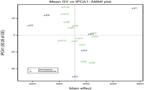
The AMMI 1 biplot of the main effect (genotype and environment effects) and IPCA-1 scores are plotted against each other (Figure 1). The score and sign of IPCA1 reflect the magnitude of the contribution of both genotypes and environments to GEI, where scores near zero are characteristic of stability, whereas a higher score (absolute value) considered as unstable and specific adapted to the environment (Crossa, 1990; Sanni et al., 2009).

The AMMI1 biplot (Figure 1) showed that G3, G4, G6, and G2 were higher yielding over the average grain yield while G13, G12, G9, and G10 had below-average grain yield. From these genotypes G13 followed by G12 were the least yielding genotypes. Among the tested genotypes G6, G2, G10, and G12 had high GxE interaction effects. In contrast, G3 and G4 had lower G×E interaction. By the same token, environment E1 (Assosa2017) had the highest grain yield. Environments E1 (Assosa2017), E3 (Bako2018), and E4 (Bonga2018) also had above-average grain yield; however, E5 (Tepi2017), E2 (Assosa2019), and E6 (Tepi2019) had below-average yield.

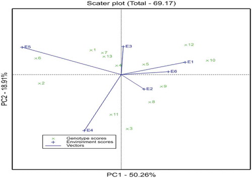
The AMMI-II biplot for grain yield display interaction of PC1 and PC2 of the tested genotypes in the six environments is presented in Figure 3. Yan and Kang (2003) reported that the distances from the biplot origin are indicative of the amount of interaction exhibited by genotypes over environments or environments over genotypes. In this figure, E6, E1, E3, and E2 with short environmental vectors, do not exert strong interactive forces and had a strong contribution to the stability of the genotype, while those with long spokes have strong interaction. As a result, environments E4 and E5 had long spokes which indicate the high discriminating ability of these environments.

Figure 1. AMMI biplot for the main effects of upland rice genotypes and environments against IPCA1 using symmetrical scaling

In addition to the environment effects, the genotypes near the origin are not sensitive to environmental interaction while those distant from the origins are sensitive and have large interaction with the environment. In this study, genotypes G3 and G4 were close to the origin and hence they are less interactive to environmental differences; however, G2, G6, G10, and 12 more responsive since they are far from the origin (Figure 2).

Figure 2. AMMI-II biplot for grain yield display interaction of PC1 and PC2 of the tested genotypes in the six environments

6. GGE biplot analysis

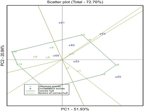
The polygon view of the GGE biplot (Figure 3.) is the best way for the identification of winning genotypes by visualizing the interaction patterns between genotypes and environments (Yan & Kang, 2003). In the GGE biplot, a polygon was formed by connecting the vertex genotypes with straight lines and the rest of the genotypes were placed within the polygon. According to Yan and Kang (2003) the vertex genotypes having the largest distance from the origin are the best or poorest in some or all environments and are more responsive to environmental change and are considered as specially adapted genotypes.

As presented in Figure 3, there are six rays which divided the biplot into seven sections. The fifth, sixth, and seventh sections did not contain environments and there is no genotype fell into section five. The first section contains genotype G11 and there is no vertex genotype for this section. The second section contains two genotypes, G3 and G4 with vertex genotype G3 which were high yielding genotypes. In the fourth section four genotypes were fell, G5, G8, G9, G10, and G12 with two vertex genotypes of G10 and G12 which were the low yielding genotypes. In this study, the partitioning of GE interaction through GGE biplot analysis showed that PC1 and PC2 accounted for 51.93% and 20.84% of the GGE sum of squares, respectively, explained 72.62% of the total variance (Figure 3).

Figure 3. The which-won-where view of the GGE biplot for the upland rice genotypes respect to the environments for grain yield

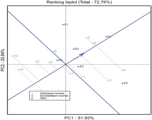
The ranking of genotypes based on mean and stability performance is presented in Figure 4. In GGE biplot analysis, the estimation of yield and stability of genotypes were done by using the average environment (tester) coordinate (AEC) methods (Yan, 2001; Yan et al., 2001). The line passing through the biplot origin is called the average environment (tester) coordinate (AEC), which is defined by the average PC1 (mean yield) and PC2 (stability) scores for all environments (Yan & Kang, 2003). Closer to the concentric circle indicates a higher mean yield. For selection, the ideal genotypes are those with both high mean yield and high stability. In the biplot, they are close to the origin and have the shorter vector from the AEC. Genotypes on the right side of the line with no arrow have yield performance greater than mean yield and the genotypes on the left side of this line had yields less than mean yield. In this study, genotypes G4 and G3 followed by G6 were the most stable and high yielding genotypes.

Figure 4. GGE biplot showing the ranking of genotypes for both grain yield and stability performance over environments

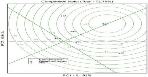
The GGE biplot comparison of genotypes relative to the ideal genotype is presented in Figure 5. In this GGE biplot, the first two PCAs captured 72.76% (PCA1 = 51.93, PCA2 = 20.84) of the GGE variance. In this figure, the ideal genotype is represented by the small concentric circle and characterized by high mean yield (PC1) and less GE interaction or high stability (PC2). Genotypes that are close to the ideal genotype are more desirable, while those far from it would not be high yielding and stable (Yan & Tinker, 2006). As a result, G4 followed by G3 and G6 were more suitable to the testing environments. On the other hand, other genotypes like genotype G12, G10, and G13 were far from the ideal genotype and considered as undesirable.

Figure 5. GGE biplot for comparison of the genotypes with respect to the ideal genotype

7. Conclusion and recommendation

The presence of genotype x environment interactions (GEI) complicates the selection of genotypes. Effective selection of genotypes for production should consider both the agronomic performance and yield stability of genotypes so as to reduce the effect of GEI. The present study revealed that the main effects, genotype, location, years and the three-way (G X L X Y) interaction effects differed significantly for the measured traits. This would indicate the wide variability in the test locations and a different response of the genotypes in different locations. The significant AMMI analysis also demonstrated the presence of G x E interactions and explained 69.17% of the G×E variance, while GGE captured 72.76% of the GGE variance.

AMMI and GGE biplot analysis showed that genotype G4 (Hidassie) followed by G3 (NERICA-4) were the most stable and high yielding genotypes among the tested 13 upland rice varieties. As a result, these varieties can be recommended for production in the testing sites and also in similar agro-ecological upland rice-producing areas of Ethiopia.

Acknowledgments

The authors are grateful to the Ethiopian Institute of Agricultural Research through Fogera national rice research and training center for financial support. In addition to this, Assosa Tepi, Bako, and Bonga research centers are highly acknowledged for executing the experiment with great responsibility.

Additional information

Funding

The authors received no direct funding for this research.

Notes on contributors

Zelalem Zewdu

The researchers who are involved in this study are from different research centers and institutes working on rice. Researchers do on evaluation, selection, and recommendations of different rice genotypes/varieties targeting the constraints of upland rice production in Ethiopia. The group is doing on many problems of upland rice variety considering the better adaptability, tolerant to disease and insect pests, grain yield, and other merits required by the end users in different areas of the country.

References

- Abebaw, D. (2018). Cereal crops research achievements and challenges in Ethiopia. International Journal of Research Studies in Agricultural Sciences., 4(6), 23–13 DOI:10.20431/2454-6224.0406003.
- Astewl, T. (2010). Analysis of rice profitability and marketing chain: The case of Fogera woreda, South Gondar Zone, Amhara National Regional State, Ethiopia [MSc Thesis]. Department of Agricultural Economics, Haramaya University.
- Comestock, F., & Moll, M. (1963). A comparison of univariate and multivariate methods to analyze environments. Field Crops Research, 56, 271–286.
- Crossa, J. (1990). Statistical analysis of multi-location trials. Advances in Agronomy, 44, 55–85.
- CSA (Central Statistical Agency). (2011). Report on area and production of major crops (Private Peasant Holdings, Meher Season) The Federal Democratic Republic of Ethiopia Central Statistical Agency Agricultural Sample Survey. ADDIS ABABA.
- Dogara, A. M., & Jumare, A. I. (2014). Origin, distribution and heading date in cultivated rice. International Journal of Plant Biology & Research, 2, 2–6.
- FAO. (2014). (Food and Agriculture Organization of the United Nations Statistics division).
- Gauch, H. G. (1992). Statistical analysis of regional yield trials: AMMI analysis of factorial designs. Elsevier.
- Gauch, H. G., & Zobel, R. W. (1996). AMMI analysis of yield trials. In M. S. Kang & H. G. Gauch (Eds.), Genotype-by-Environment Interaction (pp. 85–122). Boca Raton CRE CRC.
- Gebey, T., Berhe, K., Hoekstra, D., & Bogale, A. (2012). Rice value chain development in Fogera woreda based on the IPMS experience. ILRI.
- Girma, C. (2018). Genotype x environment interaction and yield stability in improved rice genotypes (Oryza sativa l.) tested over different locations in Western Oromia, Ethiopia. Journal of Biology, Agriculture and Healthcare, 8(12), 2018. 2224–3208 (Paper) 2225-093X (Online).
- MoARD. (2010). National rice research and development strategy of Ethiopia (The Federal Democratic Republic of Ethiopia, Ministry of Agriculture and Rural development). Addis Ababa. p. 48.
- Muthayya, S., Sugimoto, J. D., Montgomery, S., & Maberly, G. F. (2014). An overview of global rice production, supply, trade, and consumption. Annals of the New York Academy of Sciences, 1324(1), 7–14. https://doi.org/10.1111/nyas.12540
- Naroui Rad, M. R., Abdul Kadir, M., Rafii, M. Y., Hawa, Z. E., & Jaafar, F. A. (2013). Genotype x environment interaction by AMMI and GGE biplot analysis in three consecutive generations of wheat (Triticum aestivum) under normal and drought conditions.
- Payne, R. W., Murray, D. A., Harding, S. A., Baird, D. B., & Soutar, D. M. (2009). An introduction to GenStat for Windows (12th ed.). VSN International, the Waterhouse Street.
- Sanni, K. A., Ariyo, O. J., Ojo, D. K., Gregorio, G., Somado, E. A., Sanchez, I., Sie, M., Futakuchi, K., Ogunabayo, S. A., Guel, R. G., & Wopereis, M. C. S. (2009). Additive main effects and multiplicative interaction analysis of grain yield performance in rice genotypes across environments. Asian Journal of Plant Sciences, 8(1), 48–53. https://doi.org/10.3923/ajps.2009.48.53
- Sewagegne, T., Taddesse, L., Mulugeta, B., & Mitiku, A. (2013, March). Genotype by environment interaction and grain yield stability analysis of rice (Oryza sativa L.) genotypes evaluated in north western Ethiopia. Net Journal of Agricultural Science, 1(1), 10–16.
- Untung, S., Wage, R., Johnson, S. B., & Ali, J. (2015). GGE biplot analysis for genotype x environment interaction on yield trait of high fe content rice genotypes in Indonesian irrigated environments.
- Yan, W. (2001). GGE biplot a windows application for graphical analysis of multi- environment trial data and other types of two-way data. Agronomy Journal, 93(5), 1111–1118. https://doi.org/10.2134/agronj2001.9351111x
- Yan, W. (2016). Analysis and handling of G x E in a practical breeding program. Crop Science, 56(5), 2106–2118. https://doi.org/10.2135/cropsci2015.06.0336
- Yan, W., Hunt, L. A., Sheng, Q., & Szlavnics, Z. (2001). Cultivar evaluation and mega-environment investigation based on the GGE Biplot. Crop Science, 40(3), 597–605. https://doi.org/10.2135/cropsci2000.403597x
- Yan, W., & Kang, M. S. (2003). GGE biplot analysis: A graphical tool for breeders, geneticists and agronomists (1st ed.). CRC Press LLC.
- Yan, W., & Tinker, N. A. (2006). Biplot analysis of multi-environment trial data: Principles and applications. Canadian Journal of Plant Science, 86(3), 623–645. https://doi.org/10.4141/P05-169
- Zobel, R. W., Wright, M. J., & Gauch, H. G. (1988). Statistical analysis of a yield trial. Agronomy Journal, 80(3), 388–393. https://doi.org/10.2134/agronj1988.00021962008000030002x