Income inequality and its decomposition among farm households in Punjab

Abstract

Income distribution is found to be highly skewed among farm households with a Gini coefficient of 0.48. Most of the marginal and small farm households are in lower-income strata. Higher participation in pluriactivity and the highest Gini coefficient within each farm size category for marginal (0.50) and small farm size category households (0.45) highlight the tug of war for survival. Regression analysis revealed that less-educated and resource-poor farmers engaged themselves more in non-agricultural and unorganised sources of income, i.e., wages and non-farm business. Source-wise decomposition revealed that livestock and casual wages decrease income inequality. Hence, small holder farmer-centric farming systems and crops, low interest rate loans for women engaged in livestock rearing, agro-processing units and skill development centres to increase the share of non-farm income in total income are the key policy interventions.

Keywords:

• Income sources
• Income inequality
• Lorenz curve
• Gini coefficient
• Gini decomposition

Public Interest Statement

Everyone is well acquaintance with the distress the inequality cause among masses. Among all the inequalities, the inequalities of income can be considered as root cause which increase overall social inequalities. In rural agricultural economies with agriculture as a major source of income, the distress faced by marginal and small farmers is enormous. The situation for landless farmers and agricultural labourers is even more worrisome. Low income, less employment opportunities and high incidence of poverty is commonly observed among these households. Food insecurity among these households needs immediate redressal. In long term, we need to focus on capacity building programmes to ensure that their heirs have necessary skill-set which can help them to earn decent incomes.

The income of the agricultural households of Punjab has been the highest in the country at Rs 23,133, almost three times the national average of Rs 8931 for the year 2016 (Department of Economic Analysis & Research, National Bank for Agriculture and Rural Development 2018). It became possible due to inception of green revolution technologies, infrastructure development and the policies accompanying it. However, green revolution not only increased productivity but also brought income inequality among agricultural households (Dasgupta, 1977; Dhanagare, 1988; Gahukar, 1992; Pisani, 2006). Marginal and small farmers gained relatively less from the green revolution (ISI, 1975; Saini, 1976) as they had lesser marketable surplus rather than realizing lower real income due to inflation caused by higher purchasing power of the large farmers (ISI, 1975). Small farms were resource-constrained to make long-term investments and to use high productivity inputs extensively (Dasgupta, 1977; Dhanagare, 1988; Gahukar, 1992). On the contrary, the big farmers who invested and managed farms themselves were more productive than small farmers (Pisani, 2006). After the economic reforms of 1991, the situation has even worsened. Around 90 per cent farmers in the state were found to be indebted as the farm income was insufficient to meet the farm and domestic expenditure (Singh et al., 2014, 2008). Agricultural policies ignored farmers’ well-being until farm distress became a common phenomenon (Narayanamoorthy, 2017).

Inequality estimates are important for policy issues as they have a negative impact on economic growth (OECD, 2015). Higher-income inequality leads to lower aggregate demand as higher income groups have lower propensity to consume than lower-income groups. It adversely affects the confidence of people in government and increases corruption and nepotism (OECD, 2015). The households in lower-income groups find it difficult to stay healthy and accumulate physical and human capital which, in turn, affects growth (Galor & Omer, 2004). They find it difficult to lead good life (Silber, 2020).

A society comprises several subgroups, namely, rural, urban, business, agriculture, service, etc. The agriculture sector is an important subgroup within the rural economy which provides employment to a large number of people. The studies based on subgroups provide useful insights into factors contributing to inequality and provide possible solutions to minimize them. In India, the agricultural sector provides employment to 64.10 per cent rural workforce and contributes 39.20 per cent share in rural Net Domestic Product (A Singh et al., 2011). Likewise, for the overall economy, the agriculture sector contributes 14.33 per cent to the total Gross Value Added (GVA) and engages 44 per cent workforce in the year 2018–19 Ministry of Statistics and Programme Implementation, National Statistcal Office, Government of India 2020). Despite low contribution to overall GVA, agriculture is the most important component of the economy as it provides employment to a large segment of the population and provides raw material to industries.

The information about various sources of the income and extent of inequality among farm households is beneficial to orient activities for the welfare toward the vulnerable farmers in the state. Most of the studies on income distribution of rural population have been conducted at the national level (Birthal et al., 2014; Chakravorty et al., 2016; Ranganathan et al., 2016). There has been a dearth of studies on income inequality exclusively dealing with the farm households with focus on different farm -size categories (Kaur & Singh, 2014). Considering the facts discussed above, the present study focused on source-wise income inequality and its determinants among farm households. Specific objectives of the study are i) share of different sources of income in total income, ii) extent of income inequality and its source-wise decomposition and iii) determinants of income share of different sources of income among farm households in Punjab.

1. Data and descriptive statistics

This study is based on data obtained from National Sample Survey Organization (NSSO) 70^th round ‘Situation Assessment Survey of Agricultural Households’ (Ministry of Statistics and Programme Implementation, National Statisitcal Office, Government of India 2016). The data pertained to the agricultural year 2012–13. The number of sample villages and number of agricultural households surveyed by NSSO in Punjab were 94 and 725, respectively. In the survey, the household with an annual earning income of at least Rs 3000 from agriculture and allied activities was considered agricultural household. Farm households were selected among agricultural households where at least one member of the household was actively engaged in crop production. There were 558 farm households covered in Punjab during the NSSO survey. Some extreme values were dropped to obtain reliable estimates, and the final sample of the study was 553 farm households. The income estimates have been computed using the appropriate weights (provided by NSSO). Furthermore, equalized monetary value of household income was suggested for inequality studies (Buhmann et al., 1988), and therefore, equalized per capita income estimates were obtained using the square root equivalence scale to obtain income inequality estimates (Deaton, 2003). The income of the households with negative income was considered zero to generate inequality estimates, and it was given small positive value e (e = 10⁻¹⁰) to facilitate computation following (Bellu & Liberati, 2006.

Farm household income was calculated as the sum of the income from crop cultivation, livestock, regular wages and salaries, casual wages and non-farm business. Income from crop cultivation included the income earned from crops including the value of the by-products minus the paid-out cost incurred on crop cultivation. Livestock income comprised the income a household earns from sale of various livestock products after deducting maintenance expenditure. The income derived by any household member employed anywhere other than own household enterprises (agriculture, manufacturing and services sector) and receiving regular wages and salaries were categorised under regular wage and salary groups. The income earned by any household member by casual employment outside the household enterprises was defined as income from casual wages. It included the wages received in agriculture, construction and other miscellaneous sectors. The income derived by any household member by engaging himself in non-farm business activities such as hotels, restaurants, transport, construction and manufacturing was considered as non-farm business. Earlier studies based on the NSSO 70^th round have treated casual wage and regular wage/salary as single income source. But both these income sources are affected by individuals’ education level and set of skills and have opposite outcomes (Lanjouw, 2007). Similarly, the amount of income generated from these sources also had a lot of difference. Hence, both income sources were treated separately in the present study.

2. Empirical method

Quintile groups are formed to examine income distribution among farm households. Estimates of income inequality coefficients are obtained using the Gini coefficient. The Gini coefficient is a desirable indicator for inequality as it satisfies all the properties of an ideal inequality measure and also facilitates decomposition of inequality index by income sources. The value of the Gini coefficient lies between 0 and 1. The higher value of the coefficients signifies high inequality,

$G=\frac{2cov[y,f(y)]}{\bar{y}},$

whereG is the Gini coefficient of total income,

y is the total income,

f(y) is the cumulative distribution of income and

$\bar{y}$ is the mean income of the sample.

There were five income sources in the present study, i.e., crops, livestock, casual wage, regular wage and salary and non-farm business. The contribution of each income source and its effect on total income distribution are obtained by the vertical decomposition of income inequality (Lerman & Yitzhaki, 1985). It decomposes total income inequality into different sources according to their relative contribution. It provides various coefficients S_k, G_k and R_k, in which S_k represents the share of source k in total income and the coefficient obtained depicts the importance of the income source with respect to total income; G_k is the source Gini which corresponds to the distribution of income from source k, and its coefficient quantifies the inequality caused by given income sources in total inequality; and R_k is the Gini correlation which gives the correlation between distribution of income from source k and the distribution of total income indicating how a given income source is correlated with the total income of a household,

$G_K=2\ast CoV\left(\frac{Y_k{F}_k}{{\bar{Y}}_k}\right),$

$R_K=\frac{CoV(Y_k,F)}{CoV(Y_k,F_k)},$

where ${\bar{Y}}_k$ is the mean income from income source k, CoV (Y_k, F_k) is the covariance between income component k and its cumulative distribution and CoV (Y_k, F) is the covariance between income component k and cumulative distribution of the total income.

Furthermore, using the Gini decomposition by income source, the effect of changes in a particular component on inequality can be estimated, holding income constant for all other sources. Assuming a change in each household’s income from source k equal to e_k, where e is close to 1, the partial derivative of the Gini coefficient with respect to a percentage change e in source k will be

$\frac{\mathrm{\partial }G}{\mathrm{\partial }{e}_k}=S_k(G_k{R}_k-G).$

Then, the marginal effect of the income source relative to the overall Gini coefficient can be obtained by dividing by overall Gini coefficient (G) as follows:

$\frac{\mathrm{\partial }G/\mathrm{\partial }e}{G}=\frac{{\mathrm{S}}_{\mathrm{k}}{\mathrm{G}}_{\mathrm{k}}{\mathrm{R}}_{\mathrm{k}}}{\mathrm{G}}-{\mathrm{S}}_{\mathrm{k}}.$

Robustness of the marginal effect is examined using the bootstrapping technique which helped to obtain reliable stand error for the statistics. In the present study, the Gini coefficient and vertical decomposition are calculated using the Stata 12 software. Weighted linear regression analysis is conducted to determine the factors affecting the share of income source in total income. The households with no income share from the income source are dropped from the respective regression analyses. Share of the source in total income has been taken as a dependent variable, and independent variables are operational holdings (ha), proportion of leased-in land, number of workers, proportion of female workers, age (years) and education of the household head and access to institutional credit (if credit availed, then yes otherwise no). The regression equation is

Y_i =β x_i+µ_i,

where Y_i is a dependent variable, β is a vector of parameters and x_i pertains to a vector of explanatory variables.

3. Income sources of farm households

3.1. Pluriactivity among farm households

Pluriactivity is defined as the participation of members of a farm household in more than one income earning activity either on-farm or off-farm in order to increase livelihood security of the household. The farm households were tabulated according to the number of income sources of the household (Table 1). Most of the farm households are earning income from two sources (72.51%), i.e., crop and livestock income. There are around 23 per cent farm households having three or more income sources. Only 4.16 per cent households have been dependent on single source of income. Across different farm size categories, the households with operational holding greater than two hectares are mainly dependent on two income sources only (more than 80%). For households with

Table 1. Distribution of farm households according to multiplicity of income sources, Punjab (per cent)

Income sources	Farm size categories					Overall
	Marginal	Small	Semi-medium	Medium	Large
One	3.70	7.04	4.85	0.85	-	4.16
Two	53.70	64.79	84.24	80.51	85.00	72.51
Three	38.89	26.06	10.30	16.95	15.00	21.52
Four or more	3.70	2.11	0.61	1.69	-	1.81

Source: Authors’ estimates from NSSO data

smaller holdings (<2 ha), a lot of variation in the number of income sources has been observed. In marginal category, 53.70 per cent households have two income sources, 38.89 per cent households have three income sources and a few households even have four income sources also (3.70%). Similarly, in small farm size category, 64.79 per cent farm households have two income sources, 26.06 per cent households have three income sources and 2.11 per cent households have four income sources. On the contrary, income sources of most of the larger households (>2 ha) are less diversified, i.e., two income sources only.

3.2. Participation of farm households in different income sources

As the study is based on the income of farm households, thus, all the households across different farm size categories participated in crop production. The next important source of income is livestock rearing adopted by 94.00 per cent of the households (Table 2). Regular wage and salary is the source of income of 22.17 per cent households followed by non-farm business (10.67%). There are few farm households engaged in casual work (3.16%). It is observed from Table 3 that the participation in agricultural activities, i.e., crops and livestock, is somewhat uniform across different farm size categories, while participation in non-agricultural activities i.e., casual wage, regular wage and salary and non-farm business, varied across different farm size categories. As reported earlier (Ohno et al., 2021), casual wages are prevalent only in the marginal farm size category (6.62%). Participation for regular wage and salary and non-farm business declined with the increase in farm size. It can be concluded that the sources of income of marginal and small farm-households is more diversified than all other farm size categories as also observed earlier (Subramanian, 2018).

Table 2. Category-wise extent of participation of farm households in different income sources, Punjab (per cent)

Sources of income	Farm size categories					Overall
	Marginal	Small	Semi-medium	Medium	Large
Crops	100.00	100.00	100.00	100.00	100.00	100.00
Livestock	94.00	90.27	88.01	99.70	100.00	93.34
Casual wages	6.62	1.01	0.27	0.02	-	3.16
Regular wage/salary	30.50	15.04	16.46	16.32	4.75	22.17
Non-farm business	13.77	15.63	7.54	2.24	2.39	10.67

Source: Authors’ estimates from NSSO data

Table 3. Level of income of the farm households across different farm size categories, Punjab (Rs/household/annum)

Income sources	Farm size categories					Overall
	Marginal	Small	Semi-medium	Medium	Large
a) Crops	55,087 (39.69)	148,364 (71.85)	269,561 (79.03)	433,123 (84.00)	911,924 (93.03)	195,411 (71.88)
b) Livestock	24,799 (17.87)	6448 (3.12)	16,039 (4.70)	24,170 (4.69)	52,322 (5.34)	20,433 (7.52)
c) Casual wage	3216 (2.32)	780 (0.38)	68 (0.02)	19 (0.00)	0 (0.00)	1576 (0.58)
d) Regular wage/salary	43,690 (31.48)	41,468 (20.08)	47,509 (13.93)	50,482 (9.79)	8861 (0.90)	44,493 (16.37)
e) Non-farm business	12,005 (8.65)	9419 (4.56)	7919 (2.32)	7857 (1.52)	7172 (0.73)	9962 (3.66)
Total (a +b +c +d +e)	138,797 (100.00)	206,479 (100.00)	341,097 (100.00)	515,651 (100.00)	980,279 (100.00)	271,875 (100.00)

Source: Authors’ estimates from NSSO data

Source-wise distribution of per capita income into quintile groups

4. Income and its distribution among farm households

4.1. Level of income

The average income of the farm household in Punjab is estimated to be about 2.72 lakh per annum. The main source of income is crop cultivation (71.88%), followed by regular wage and salary (16.37%), livestock (7.52%), non-farm business (3.66%) and casual wage (0.58%; Table 4). Across different farm size categories, the annual income is Rs 1.39 lakh, Rs 2.06 lakh, Rs 3.41 lakh, Rs 5.16 lakh and Rs 9.80 lakh for marginal, small, semi-medium, medium and large farm-size categories, respectively. The share of income from crop cultivation increased with the increase in farm size. It is 39.69 per cent for marginal, 71.85 per cent for small, 79.03 per cent for semi-medium, 84.00 per cent for medium and 93.03 for large farm households. Livestock contributed, on average, 7.52 per cent to the total farm income, which increased with the increase in the farm size among different farm size categories with the exception of marginal farm households where it contributed around 18 per cent to the total income. The per cent share of casual wages, regular wage and salary and non-farm business showed an inverse relationship with farm size categories. Regular wage/salary contributed the most (31.48%) in the total income of the marginal farm households, while its share in income of large households was almost negligible (0.90%). Similarly, the per cent share for non-farm business was 3.86 per cent. It also contributed significantly to the income of marginal farm households (8.65%) and insignificantly to large farm size households. Casual wages formed less than one per cent of average annual income of all farm households, and it is the highest for marginal farm size category (2.32%).

Table 4. Distribution of per capita income of farm households into quintile groups, Punjab

Quintiles	Income sources (%)					Average annual income (Rs/capita)
	Crops	Livestock	Casual wage	Regular wage and salary	Non-farm business
Bottom	80.97	−23.29	4.19	23.29	14.84	7461 (100.00)
Q2	53.70	13.98	2.71	19.86	9.75	25,902 (100.00)
Q3	83.09	11.38	0.51	1.80	3.22	44,165 (100.00)
Q4	77.35	8.66	-	11.88	2.11	70,824 (100.00)
Top	70.24	6.75	0.03	20.93	2.06	145,468 (100.00)
Overall	71.88	7.52	0.58	16.37	3.66	51,825 (100.00)

Source: Authors’ estimates from NSSO data

Source-wise annual per capita income of the farm households has been presented in five quintiles which varied a lot across different income sources. There is a huge difference in income of the top and bottom quintiles. The income of the top quintile is 20 times higher than the bottom quintile. In the bottom quintile, the average annual income of the farm households is Rs 7461 per capita (Table 3), out of which 80 per cent are from cultivation of crops, followed by regular wage and salary (23.29%), non-farm business (14.84%) and casual wage (4.19%). The income from livestock is negative (−23.29%) in the bottom quintile. It highlights the findings where importance of herd size and quality of the livestock for positive returns in livestock were thoroughly discussed (Gehrke & Grimm, 2014). In the second quintile, the average income is more than three times higher than the bottom quintile. It has been Rs 25,902 on per capita basis in which the share of crop cultivation is 53.70 per cent, followed by regular wage and salary (19.86%), livestock (13.98%), non-farm business (9.75%) and casual wage (2.71%). The average income of the third quintile is 1.5 times higher than that of the second quintile. The average annual income is Rs 44,165 per capita in which 83.09 per cent is from crop cultivation, followed by livestock (11.38%), non-farm business (3.22%), regular wage and salary (1.80%). Following the same trends, the average income of the fourth quintile is almost double of the third quintile. The per capita annual income has been Rs 70,824 with the highest share from crop cultivation (Rs 77.35%), followed by regular wage and salary (11.88%), livestock (8.66%) and non-farm business (2.11%). The average income of the top quintile is double that of the fourth quintile. It has been Rs 1.45 lakh on the per capita basis in which 70.24 per cent share is from crop cultivation, followed by regular wage and salary (16.37%), livestock (7.52%) and non-farm business (2.11%). The income from casual wage is negligible in third, fourth and top quintiles. Except Q1, the share of income from livestock decreased in successive quintile groups. Regular wage and salary has significant share in the income of top two quintiles. The income is highly unequally distributed among the farm households belonging to different income quintiles.

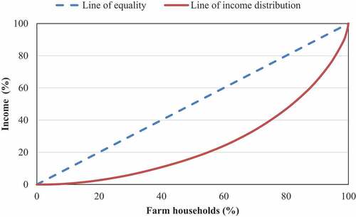
The Lorenz curve is plotted for total income earned by the farm households and depicts disproportionate distribution (Figure 1). The lower decile group has less than one per cent share in total income. Similarly, the bottom 20 per cent have only 2.65 per cent share in total income. It clearly shows highly skewed income distribution among farm households. The lower 40 per cent of the farm households have access to 10.83 per cent of the total income among farm households. The bottom 60 per cent farm households have around 24 per cent share in total income distribution. The upper decile population of the farm household in Punjab has access to around 35 per cent income, and upper 20 per cent of the farm households have 52.98 per cent share in the total income depicting unequal distribution.

Figure 1. Distribution of farm households according to their income.

5. Decomposition of income inequality

5.1. Source-wise decomposition of income inequality among farm households

Decomposition of income inequality across different income sources has been estimated to examine the sources of income inequality among farm households (Table 5). The Gini coefficient obtained is 0.48, depicting high income inequality among farm households. The findings are in line with the previous studies reporting high income inequality in rural Punjab (Vatta and Pavithra 2016; Choudhary & Singh, 2019). The decomposition analysis revealed that the Gini coefficient for each individual income source is the highest for casual wage (0.98). It is due to lesser participation of farm households in this income source. Only marginal farmers worked as casual workers. The Gini coefficient is also high for regular wage and salary and non-farm business income. Crop production contributed the most (0.82) to the overall Gini coefficient. Bathla and Kumar (2019) have also reported the highest contribution of operated land in total income inequality in Punjab (68.93%) which can be considered proxy to crop production. It is followed by regular wage and salary (0.10), livestock (0.06) and non-farm business (0.02). The marginal contribution of livestock and casual wage to the overall Gini coefficient is negative and significant, indicating them as income inequality decreasing sources. These findings on the inequality decreasing effect of livestock have been well established in the literature (Adams & He, 1995; Birthal et al., 2002; Choudhary & Singh, 2019; IEG, 2015). Similarly, the income inequality decreasing effect of casual labour has been well established as the main recipients of this income source, which belongs to the lower tail of income distribution (Lanjouw, 2007; Ranganathan et al., 2016; Shariff & Azam, 2009). Overall, the share of the rural non-farm sector in the income of the farm households was minimal. These sources have been identified as inequality decreasing sources (Adams & He, 1995; Lanjouw & Shariff, 2004; Himanshu, Lanjouw et al., 2013; Pavithra & Vatta, 2013; Birthal et al., 2014. Punjab can learn from China’s rapid growth of rural enterprises which was the only contrasting factor between India-China rural growth stories (Gulati & Fan, 2008).

Table 5. Income inequality among farm households and its source-wise decomposition, Punjab

Income sources	Income share	Source Gini	Proportional contribution to Gini	Marginal contribution to Gini
Crops	0.820	0.534	0.824	0.005 (0.0147)
Livestock	0.101	0.641	0.052	−0.049 (0.0049)**
Casual wages	0.005	0.979	−0.005	−0.010 (0.0029)**
Regular wages and salary	0.085	0.929	0.099	0.014 (0.0110)
Non-farm business	0.027	0.961	0.023	−0.004 (0.0051)
Total income	-	0.482	-	-

Source: Authors’ estimates from NSSO data

Note: Bootstrapped standard errors with 1000 replications in parentheses,

**significant at the 1% level of significance

5.2. Decomposition of income inequality within different farm size categories

Each farm size category has different sources of income depending upon resource endowment, risk taking behaviour, education level of the family members and family composition, so income distribution within each farm size category is also expected to vary a lot. Hence, farm size category-wise decomposition of income inequality is analysed to see the pattern of income distribution within each farm size category. There is a lot of variation in income inequality for each farm size category. The Gini coefficient is 0.50, 0.45, 0.38, 0.31 and 0.40 for marginal, small, semi-medium, medium and large farm households, respectively (Table 6). The income inequality estimates for marginal and small farm households are very high, thus contradicting earlier findings of lesser income inequality (Kaur & Singh, 2014). While decomposing the income inequality among marginal farm households, the share of regular wages and salary source in overall Gini coefficient is the highest (0.36), followed by crops (0.28) and livestock (0.27). The share of non-farm business (0.07) and casual wages (0.01) contributed very little to overall inequality. The marginal effect of income inequality (elasticity) is significant and negative for income from crop cultivation and casual wage and positive for regular wage and salary. For small farm households, the decomposition revealed that contribution of crop income in Gini coefficient is the highest (0.62) followed by regular wage and salary (0.29). The coefficient of income inequality elasticity is significant for crop, livestock and regular wage and salary. The coefficients are negative for crop and livestock income, depicting the inequality decreasing effect of these sources, while positive for regular wage and salary, depicting the inequality increasing effect of this income source. The number of semi-medium and medium operational holdings is on the rise in Punjab (Department of Agriculture and Cooperation, Government of India 2016). Interestingly, the inequality is least for the households belonging to both these farm-size categories. The extent of inequality has been moderate for large farm households. The overall inequality decreasing effect of the livestock sector is reported in Punjab as found in other regions of India (Birthal et al., 2014; Pavithra & Vatta, 2013; Ranganathan et al., 2016) as well as all around the world (Adams & He, 1995; Lanjouw & Shariff, 2004).

Table 6. Decomposition of income inequality within farm households across different farm size categories in Punjab

Farm size categories	Income sources	Income share	Source Gini	Proportional contribution to Gini	Marginal contribution to Gini
Marginal	Crops	0.393	0.570	0.278	−0.115 (0.048)*
	Livestock	0.263	0.716	0.267	0.004 (0.040)
	Casual wage	0.049	0.924	0.013	−0.036 (0.016)*
	Regular wage/salary	0.258	0.889	0.360	0.103 (0.051)*
	Non-farm business	0.077	0.928	0.070	−0.007 (0.020)
	Total income	-	0.498	-	-
Small	Crops	0.739	0.456	0.616	−0.123 (0.058)*
	Livestock	0.098	0.652	0.050	−0.048 (0.011)**
	Casual wage	0.004	0.988	-	−0.004 (0.007)
	Regular wage/salary	0.173	0.924	0.288	0.115 (0.045)*
	Non-farm business	0.048	0.944	0.060	0.012 (0.014)
	Total income	-	0.454	-	-
Semi-medium	Crops	0.854	0.379	0.754	−0.010 (0.046)
	Livestock	0.109	0.607	0.071	−0.038 (0.013)**
	Casual wage	0.001	0.994	−0.002	−0.002 (0.002)
	Regular wage/salary	0.064	0.944	0.115	0.052 (0.029)
	Non-farm business	0.014	0.978	0.022	0.008 (0.008)
	Total income	-	0.379	-	-
Medium	Crops	0.893	0.303	0.793	−0.100 (0.039)*
	Livestock	0.075	0.602	0.038	−0.037 (0.014)**
	Casual wage	0.001	0.992	−0.003	−0.004 (0.003)
	Regular wage/salary	0.041	0.936	0.083	0.042 (0.022)
	Non-farm business	0.022	0.972	0.059	0.036 (0.021)
	Total income	-	0.309	-	-
Large	Crops	0.934	0.403	0.933	−0.001 (0.016)
	Livestock	0.050	0.432	0.017	−0.033 (0.016)*
	Casual wage	-	-	-	-
	Regular wage/salary	0.014	0.925	0.027	0.013 (0.009)
	Non-farm business	0.010	0.950	0.016	0.006 (0.010)
	Total income	-	0.402	-	-

Source: Authors’ estimates from NSSO data

Note: Bootstrapped standard errors with 1000 replications in parentheses

**significant at the 1% level of significance

* significant at the 5% level of significance

6. Determinants of access of farm households to different income sources

This section deals with determinants of farm households’ access to different income sources. There are a large number of factors that lead to diversification of income sources for different farm households. Important factors have been identified and highlighted by various researchers (Barrett et al., 2001; Birthal et al., 2014). Various push factors include higher risk in agriculture, diminishing returns to input use, excess labour supply with respect to land availability and market imperfection in land, labour and credit markets. Regression estimates were worked to identify factors affecting the share of different sources of income in total income of the farm households. Share of income source in total income has been taken as the dependent variable, while the independent variables include operational holdings; proportion of leased-in land; total number of workers in a farm household; proportion of female workers in total workers; access to institutional credit and age, sex and education of the head of the household. Descriptive statistics of the explanatory variables are presented in Table 7. There is no doubt that land is an important variable which determines the income share of different sources in total income. The average size of the land holdings of the sample is 3.18 ha. The leased-in land comprised 18 per cent of the operated area. The average number of workers in a family is 3.63 members. The income source in which household engages depends upon the gender composition of the workers. The share of female workers to total workers for the sample is 47 per cent. Age is taken as proxy of the working capacity as it affects employment choices. The average age of the household head is 54.76 years for the farm households. Around 94 per cent of the farm households in Punjab are headed by males. Unskilled and less-educated persons were expected to be engaged in low paid job opportunities. The access to institutional credit is taken as proxy for availability of external finances. As most of the investments require high start-up capital and have a slow rate of returns over investment, it is assumed that external finances can boost or impede

Table 7. Descriptive statistics of the variables used in regression

Variables	Mean	Standard deviation
Operational holding size (ha)	3.18	3.38
Leased-in land (proportion in land possessed)	0.18	0.30
Total workers (age 15–59) (no.)	3.63	1.70
Female workers (proportion in total workers)	0.47	0.17
Household head age (years)	54.76	13.82
Household head gender (male)	0.94	0.24
Access to institutional credit (proportion in total)	0.60	0.49
Education
Illiterate (proportion in total)	0.33	0.47
Up to middle (proportion in total)	0.35	0.48
Secondary or higher secondary (proportion in total)	0.27	0.44
Graduate or above (proportion in total)	0.06	0.23

investment decisions. The regression estimates for access of farm households to different income sources are presented in Table 8. The income share from crops is positive and significantly associated with operational holdings, while the share of all other income sources was negatively associated with operational holdings. Labour endowment has been found to be positively associated in wages and non-farm business while negatively associated for crops, dairy and salary. This implies that the farm households with larger labour endowment look for income generation through non-agricultural sources except salaried work, where strong and positive association between higher education and proportion of income from salary in total income is observed. Similar observation on the role of education in higher non-farm income is reported by Devi and Ranganathan (2021). The present study contributes further by pin-pointing that higher education increases salary income among non-farm sources. On the contrary, the households with a lower level of education and low-resource endowment especially engage in wages and non-farm businesses and have higher income share from these sources. The proportion of female workers in total workers and proportion of livestock income in total income are positively associated. Even the female headed households and proportion of livestock income in total income are positively associated. Hence, it can be deduced that the presence of women workforce in the family increases the share of livestock income in total income of the farm households. Access to institutional credit has been positively associated with agriculture while negatively associated with livestock and non-farm business.

Table 8. The regression estimates for determinants of income share

Explanatory variables	Crops			Livestock			Wages			Salary			Non-farm business
	Coefficient	t-stat	p-value	Coefficient	t-stat	p-value	Coefficient	t-stat	p-value	Coefficient	t-stat	p-value	Coefficient	t-stat	p-value
Constant	0.066	4.81	0.000	1.228	81.94	0.000	−1.009	−163.8	0.000	0.630	122.1	0.000	−0.066	−7.40	0.000
Landholding size (ha)	0.050	65.59	0.000	−0.016	−21.17	0.000	−0.083	−48.43	0.000	−0.037	−129.6	0.000	−0.068	−118.9	0.000
Proportion of leased-in land	−0.072	−10.51	0.000	−0.071	−10.13	0.000	0.133	41.28	0.000	0.257	109.3	0.000	−0.105	−23.73	0.000
Total workers (no.)	−0.029	−12.54	0.000	−0.043	−17.78	0.000	0.035	−23.43	0.000	−0.031	−32.86	0.000	0.051	34.36	0.000
Proportion of female workers in total workers	0.006	1.64	0.102	0.046	11.68	0.000	0.503	115.7	0.000	0.141	100.1	0.000	−0.077	−32.18	0.000
Household head age (years)	0.008	52.97	0.000	−0.012	−71.71	0.000	0.005	71.54	0.000	−0.002	−38.24	0.000	0.005	57.33	0.000
Household head gender (male =1 otherwise =0)	0.055	6.58	0.000	−0.145	−16.10	0.000	-	-	-	−0.123	−39.29	0.000	0.227	52.66	0.000
Access to institutional credit (availed =1 otherwise =0)	0.259	62.94	0.000	−0.247	−57.07	0.000	0.178	81.68	0.000	−0.051	−33.27	0.000	−0.020	−7.89	0.000
Education
Up to middle (up to middle =1 otherwise =0)	0.153	31.23	0.000	−0.362	−71.44	0.000	1.024	326.9	0.000	0.044	24.17	0.000	0.262	94.79	0.000
Secondary or higher secondary (secondary or higher secondary = 1, otherwise = 0)	−0.053	−10.36	0.000	−0.011	−2.13	0.033	0.912	283.2	0.000	0.181	98.52	0.000	−0.022	−7.03	0.000
Graduate or above (graduate or above =1 otherwise =0)	−0.073	−7.02	0.514	−0.147	−12.75	0.000	-	-	-	0.182	58.49	0.000	−0.019	−2.41	0.016

7. Conclusions and policy implications

The study estimates the income inequality among the farm households and contribution of various sources to income inequality. It is well known that farm households have high economic as well as social importance in rural areas of Punjab, but further sub-classification reveals a lot of distress among the farm households belonging to marginal and small farm size categories. The distress is visible through their occupational diversity as most of the marginal and small farmers are engaged in non-agricultural activities along with agriculture. The distribution of income among farm households is highly skewed (Gini coefficient =0.48). The study has highlighted the importance of choosing the income sources carefully while studying vertical income inequality. Previous studies considered regular wages and casual wages as single income source, but this study highlighted that these sources have an opposite effect on overall income inequality. Casual wages have an income inequality deceasing effect. Regression analysis revealed that income sources are least affected by land endowment except crop income. Labour endowment increased non-farm work participation, where educated preferred salaried work, while uneducated and resource poor moved towards wages and non-farm business. Moreover, it was also observed that higher presence of female workers in a farm household increases its income from livestock production. Furthermore, farm size category-wise income inequality decomposition revealed high income inequality within marginal and small farm size categories. The positive effect of crop income on overall income distribution of marginal farm households can be augmented through policy suggestions (Kent & Poulton, 2020) like agricultural research on farming systems and crops to be conducted with focus on the needs of marginal farmers. Development of labour-intensive farming systems like fruit and vegetable production will benefit marginal farmers as it will increase availability of casual wages. Moreover, participation of marginal farmers in farmer producer organisation can be promoted in Punjab (Rangarajan & Dev, 2021). Livestock income has been identified as an important income inequality decreasing source for all the farm-size categories. Hence, strengthening of the dairy sector through the breed development program, livestock insurance and other such interventions are important policy implications of the study. Female workforce and livestock income are positively correlated, and hence, women-centric credit programs to provide low interest loans to women should be developed. The share of non-farm business in the income of the farm households is almost negligible. Their adoption among farm households should be enhanced via proper policy intervention like developing of agro-processing industries and skill development centres.

Acknowledgements

This research work is a part of dissertation titled “Income inequality among farm households in Punjab” submitted at Punjab Agricultural University, Ludhiana. Financial assistance from the Indian Council of Agricultural Research in the form of Senior Research Fellowship is highly acknowledged. The authors are thankful to Kamal Vatta (Head and Professor, Department of Economics and Sociology, Punjab Agricultural University, Ludhiana) for their support and guidance in improving this research work.

Disclosure statement

No potential conflict of interest was reported by the author(s).

Additional information

Funding

This work was supported by the Indian Council of Agricultural Research [EDN/1/25/2015/-Exam cell].

Notes on contributors

Rohit Saini

Rohit Saini is a Ph.D. in Agricultural Economics currently working as Junior Research Fellow at Department of Economics and Sociology, Punjab Agricultural University, Ludhiana, India. His research interests include status of income of the agricultural households with special reference to landless, marginal and small farmers. His special interests include addressing the income stress in rural economy and analysing the potentials of creating decent opportunities in the vicinity of the rural households.

Manjeet Kaur

Manjeet Kaur is Principal Agricultural Economist at Department of Economics and Sociology, Punjab Agricultural University, Ludhiana, India. Her area of interest includes farmers’ income, indebtedness, stress faced by agricultural households. She has extensively worked to address the problems faced by agricultural labourers in Punjab and currently working on the rural distress and cause of suicides among persons engaged in agriculture.

References

- Adams, R. H., & He, J. J. 1995. Sources of income inequality and poverty in rural Pakistan. Research report 102, International Food Policy Research Institute. https://www.ifpri.org/publication/sources-income-inequality-and-poverty-rural-pakistan
- Barrett, C. B., Reardon, T., & Webb, P. (2001). Non-farm income diversification and household livelihood strategies in rural Africa: Concepts, dynamics and policy implications. Food Policy, 26(4), 315–15. https://doi.org/10.1016/S0306-9192(01)00014-8
- Bathla, S., & Kumar, A. (2019). Factors contributing to income inequalities among agricultural households in India. Economics and Political Weekly, 54(21) , 55–61 https://www.epw.in/journal/2019/21/special-articles/factors-contributing-income-inequalities-among.html.
- Bellu, L. G., & Liberati, P. (2006). Policy impacts on inequality: Decomposition of income inequality by subgroups. EASYPol, Food and Agriculture Organization, Italy. http://www.fao.org/3/am342e/am342e.pdf
- Birthal, P. S., Joshi, P. K., & Kumar, A. 2002. Assessment of research priorities for livestock sector in India. Policy paper 15. National Centre for Agricultural Economic and Policy Research, New Delhi, India. http://citeseerx.ist.psu.edu/viewdoc/download?doi=10.1.1.615.4101&rep=rep1&type=pdf
- Birthal, P. S., Negi, D. S., Jha, A. K., & Singh, D. (2014). Income sources of farm households in India: Determinants, distributional consequences and policy implications. Agricultural Economics Research Review, 27(1), 37–48. https://doi.org/10.5958/j.0974-0279.27.1.003
- Buhmann, B., Rainwater, L., Schmaus, G., & Smeeding, T. M. (1988). Equivalence scales, well-being, inequality, and poverty: Sensitivity estimates across ten countries using the Luxembourg Income Study (LIS) database. The Review of Income and Wealth, 34(2), 115–142. https://doi.org/10.1111/j.1475-4991.1988.tb00564.x
- Chakravorty, S., Chandrasekhar, S., & Naraparaju, K. (2016). Income generation and inequality in India’s agricultural sector: The consequences of land fragmentation. Indira Gandhi Institute of Development Research. http://www.igidr.ac.in/pdf/publication/WP-2016-028.pdf
- Choudhary, B. B., & Singh, P. (2019). How unequal is rural Punjab? Empirical evidence from spatial income distribution. Current Science, 117(11), 1855–1866. https://doi.org/10.18520/cs/v117/i11/1855-1862
- Dasgupta, B. (1977). India’s green revolution. Economic and Political Weekly, 12(7) , 241–260. https://www.epw.in/journal/1977/6-7-8/specials-economic-crisis/india-s-green-revolution.html
- Deaton, A. (2003). Health, inequality and economic development. Journal of Economic Literature, 41(1), 113–158. https://doi.org/10.1257/jel.41.1.113
- Department of Agriculture and Co-operation, Government of India. 2016. All india report on number and area of operational holdings. https://agcensus.nic.in/document/agcen1516/ac_1516_report_final-220221.pdf
- Department of Agriculture, Co-operation and Farmers’ Welfare, Government of India. 2018. Agricultural Statistics at A Glance. https://agricoop.gov.in/sites/default/files/agristatglance2018.pdf
- Department of Economic Analysis & Research, National Bank for Agriculture and Rural Development. (2018). NABARD all India rural financial inclusion survey 2016-17 (Mumbai: NABARD). https://www.nabard.org/auth/writereaddata/tender/1608180417NABARD-Repo-16_Web_P.pdf
- Devi, B., & Ranganathan, T. (2021). Emerging challenges in rural non-farm sector and inequality in rural India: Insights from IHDS survey. Finance and Economics Review, 3(1), 88–101. https://doi.org/10.38157/finance-economics-review.v3i1.303
- Dhanagare, D. N. (1988). The green revolution and social inequalities in rural India. Bulletin of Concerned Asian Scholars, 20(2), 2–13. https://doi.org/10.1080/14672715.1988.10404444
- Gahukar, R. T. (1992). Green revolution in food crops: An Indian experience. Outlook on Agriculture, 21(2), 129–136. https://doi.org/10.1177/003072709202100208
- Galor, O., & Omer, M. (2004). From physical to human capital accumulation: Inequality and the process of development. The Review of Economic Studies, 71(4), 1001–1026. https://doi.org/10.1111/0034-6527.00312
- Gehrke, E., & Grimm, M. 2014. Do cows have negative returns? The evidence revisited. IZA working paper no 8525, Institute of Labour Economics, Bonn. https://www.iza.org/publications/dp/8525/do-cows-have-negative-returns-the-evidence-revisited
- Gulati, A., & Fan, S. (2008). The dragon and the elephant: Learning from agricultural and rural reforms in China and India. Issue briefs 49. International Food Policy Research Institute. https://ebrary.ifpri.org/digital/api/collection/p15738coll2/id/12385/download
- Himanshu, Lanjouw, P., Murgai, R., & Stern, N. (2013). Nonfarm diversification, poverty, economic mobility, and income inequality: A case study in village India. Agricultural Economics, 44(4–5), 461–473. https://doi.org/10.1111/agec.12029
- IEG. (2015). Farmers’ income in India: Evidence from secondary data. Agricultural Situation in India, 72(3) , 30–70. http://iegindia.org/ardl/Farmer_Incomes_Thiagu_Ranganathan.pdf
- ISI. (1975). Structural causes of the economic crisis. Economics Poltical Weekly, 10 3 , 83–86. https://www.epw.in/journal/1975/3/special-articles/structural-causes-economic-crisis.html
- Kaur, S., & Singh, G. (2014). Analysis of income distribution among marginal and small farmers in rural Punjab. International Journal of Scientific Research, 3 3 , 755–759. https://www.ijsr.net/archive/v3i3/MDIwMTMxMTk5.pdf
- Kent, R. & Poulton. (2020). Marginal farmers: A review of the literature. Centre for Development, Environment and Policy. https://agris.fao.org/agris-search/search.do?recordID=GB2013202015
- Lanjouw, P., & Shariff, A. (2004). Rural non-farm employment in India: Access, income and poverty impact. Economic and Political Weekly, 39(4429), 46. https://www.jstor.org/stable/4415616
- Lanjouw, P. (2007). Does the rural nonfarm economy contribute to poverty reduction? In Transforming the rural nonfarm economy: Opportunities and threats in the developing world. Ed S Haggblade, P. B. R. Hazell, & T. Reardon. 55–82. International Food Policy Research Institute. https://www.ifpri.org/publication/transforming-rural-nonfarm-economy-0
- Lerman, R. I., & Yitzhaki, S. (1985). Income inequality effects by income sources: A new approach and applications to the United States. The Review of Economics and Statistics, 67(1), 151–156. https://doi.org/10.2307/1928447
- Ministry of Statistics and Programme Implementation, National Statistical Office, Government of India. 2016. Income, Expenditure, Productive Assets and Indebtedness of Agricultural Households in India. http://mospi.nic.in/sites/default/files/publication_reports/nss_rep_576.pdf
- Ministry of Statistics and Programme Implementation, National Statistical Office, Government of India, New Delhi. 2020. Annual report: Periodic Labour Force Survey 2018-19. http://mospi.nic.in/sites/default/files/publication_reports/Annual_Report_PLFS_2018_19_HL.pdf
- Narayanamoorthy, A. (2017). Farm income in India: Myths and realities. Indian Journal of Agricultural Economics, 72(1), 48–75. https://ideas.repec.org/a/ags/inijae/302245.html
- OECD. (2015). In it together: Why less inequality benefits all. https://doi.org/10.1787/9789264235120-en
- Ohno, A., Fujita, K., & Vatta, K. (2021). Agrarian structure of Punjab in the post-green revolution era: Household strategies for distress coping. Economic and Political Weekly, 56(40), 56–64. https://www.epw.in/journal/2021/40/special-articles/agrarian-structure-punjab-post-green-revolution.html
- Pavithra, S., & Vatta, K. (2013). Role of non-farm sector in sustaining rural livelihoods in Punjab. Agricultural Economics Research Review, 26 2 , 257–265. https://ageconsearch.umn.edu/record/162146/files/11-Pavithra-final.pdf
- Pisani, E. (2006). Some socio-economic consequences of the green revolution. Land Reform, 2(24977) , 97–107. https://mpra.ub.uni-muenchen.de/24977/
- Ranganathan, T., Tripathi, A., & Rajoriya, B. (2016). Changing sources of income and income inequality among Indian rural households. In Sarap, Kailash, Motkuri, Venkatanarayana (eds.), National seminar on dynamics of rural labour relations. National Institute of Rural Development and Panchayati Raj (pp. 31–32) . http://nirdpr.org.in/nird_docs/srsc/srsc-pub-090518-5.pdf
- Rangarajan, C., & Dev, S. M. (2021). How FPOs can help small and marginal farmers. The Indian Express. https://indianexpress.com/article/opinion/columns/nabard-agrarian-distress-farmers-protest-farm-laws-7222830/
- Saini, G. R. (1976). Green revolution and the distribution of farm income. Economic and Political Weekly, 11(13) , A17–22. https://www.epw.in/journal/1976/13/review-agriculture-uncategorised/green-revolution-and-distribution-farm-incomes.html
- Shariff, A., & Azam, M. 2009. Income inequality in rural India: Decomposing the Gini by income sources SSRN . https://ssrn.com/abstract=1433105
- Silber, J. (ed). (2020). Economic studies in inequality, social exclusion and well-being (pp. 183186). 183186). Springer Nature. https://www.springerprofessional.de/en/economic-studies-in-inequality-social-exclusion-and-well-being/925154
- Singh, S., Kaur, M., & Kingra, H. S. (2008). Indebtedness among farmers in Punjab. Economic and Political Weekly, 43(26) , 130–136. https://www.epw.in/journal/2008/26-27/review-agriculture-review-issues-specials/indebtedness-among-farmers-punjab.html
- Singh, A., Prasanna, P. A. L., & Chand, R. (2011). Farm size and productivity: Understanding the strength of smallholders and improving their livelihoods. Economic and Political Weekly, 26(27), 5–11. https://www.epw.in/journal/2011/26-27/review-agriculture-review-issues-specials/farm-size-and-productivity
- Singh, S., Bhogal, S., & Singh, R. (2014). Magnitude and determinants of indebtedness among farmers in Punjab. Indian Journal of Agricultural Economics, 56(26) , 244–256. https://www.epw.in/journal/2021/26-27/review-rural-affairs/indebtedness-among-farmers-punjab.html
- Subramanian, S. 2018. Participation of rural households in farm, non-farm and pluri-activity: Evidence from India. Working paper 412. The Institute for Social and Economic Change, Banglore, India. http://www.isec.ac.in/WP%20412%20-%20S%20Subramanian%20-%20final.pdf