A ML-AI ENABLED ENSEMBLE MODEL FOR PREDICTING AGRICULTURAL YIELD

Abstract

Simplistic linear methods for predicting crop yield leave out important factors like climate, rainfall, soil, irrigation, and land characteristics. Recent literature points to use of individual Machine Learning (ML) and Artificial Intelligence (AI) models for better prediction of crop yield. However, such methods have not been used in the Indian context. Moreover, given the diversity of land, climate, soil and irrigation facilities in the country, it is necessary to develop an ensemble approach incorporating a significant number of ML algorithms to have a better prediction of crop yield across geographies of the country. The purpose of this paper is to: (a) develop scenario-specific algorithms for ML models and identify the best fit model for yield prediction and (b) develop an ensemble approach synthesizing the ML models for better overall prediction of crop yield in India.

Keywords:

• forecasting agricultural yield
• ensemble method
• ML models

1. Introduction

Crop yield in India is greatly influenced by vagaries of nature, specifically rainfall. Choice of wrong crops for farming or inadequate crop yield leads to farmers’ inability to repay loans and committing of suicide. The National Crime Records Bureau put the number of farming related suicides at 10,281 in 2019, accounting for 7.4% of all suicides in India (Sengupta, 2020). This warrants a robust forecasting methodology for predicting crop yield in India. Existing models for prediction primarily use rainfall and fertilizer usage data and apply linear models like regression for estimating crop yield. This leaves out important variables like sunlight, climate, irrigation, temperature variations, water level of soil, nutrient content of soil and soil profile.

There have been efforts to predict crop yield by modeling complex nonlinear relationships that exist among some of the variables. In recent times, Machine Learning (ML) and Artificial Intelligence (AI) powered forecasting systems have been used in the USA, UK, Finland and Netherlands and these systems have reported a significant reduction in forecasting error. This has helped farmers to decide on the types of crops to grow and the time horizon when to grow them.

However, ML-AI frameworks have not been used in the Indian setting. Variables other than rainfall and fertilizer usage statistics have been ignored while estimating crop yield. Major reason behind such omission is lack of uniformity of data available across different states and regions. Missing data and data lag for preceding two to three years has led to inaccurate forecasting or increase in forecasting error. The problem gets complicated with data on different variables being collected by different agencies and at different levels (e.g., district, state and national level). Method of data collection also varies across agencies and across geographies. These have proved to be impediments in applying modern approaches towards forecasting using ML-AI algorithms.

As part of ML-AI mechanism, different ML methodologies can be used and the best fit method termed as the “champion” model can be selected for prediction. But it is felt to be too generalist a system if applied to the Indian setting owing to different sets of demographics across different regions. Hence, we propose an ensemble model that incorporates all the ML methodologies applying probabilistic weights and developing a holistic framework that can be used for predicting crop yield across the entire country. Data used for this study shows that the proposed ensemble method can further improve the prediction accuracy as compared to individual ML methodologies.

The paper is organized as follows: First we present literature on methodologies for estimating crop yield and the issues faced in India in estimation. This is followed by objectives of the study. The next section presents a description of the ML tools used for estimation. The methodology section explains in detail the proposed ensemble model. The analysis section presents the model in a step-wise manner. The last section highlights the contributions of the study.

2. Methodologies for estimating crop yield

Recent studies point to use of newer methods for forecasting. Some of these are: artificial neural networks (Balaji and Dakshayinib 2018; Sellam & Poovammal, 2016), logistic regression and generalised linear model (GLM; Bakar & Jin, 2020), linear discriminant analysis (LDA; Xanthopoulos et al., 2013), support vector machine (SVM; Chen et al., 2021), classification and regression trees (CART; Loh, 2011), chi-square automatic interaction detection (CHAID; Galguera et al., 2006), naïve bayes (Singh et al., 2019), AdaBoost (Mrinalini et al., 2021), gradient boosting (Trizoglou et al., 2021) and random forest (Ramalingam & Baskaran, 2021).

Mayuri and Priya (2018) addressed the challenges of forecasting using a combination of image processing and ML tools to forecast crop yield. Image processing interchanges the role of farmers “observing” crops to check if there is insect onslaught on the crops. These are followed up by use of classification and regression models to forecast the yield of crops. Similarly, Mishra and Mishra (2015) point out that data from biological discipline is typically complex and vague and approaches using machine learning where the system generates adaptive learning techniques can aid to analyse these data better.

Gandhi and Armstrong (2016) review application of data mining techniques in the agriculture sector and present a nomenclature on how data mining can be realized from complex agricultural datasets. Beulah (2019) conducted a survey on the use of various data mining techniques for crop yield prediction and opined that better crop yield prediction can be achieved by employing new data mining techniques and approaches. Klompenburga et al. (2020) through an exhaustive literature review shed light on the mostly used machine learning algorithms used in literature. This is presented in Table 1 below:

Table 1. Mostly used machine learning algorithms

Most used machine learning algorithms	No. of times used
Neural Networks	27
Linear Regression	14
Random Forest	12
Support Vector Machine (SVM)	10
Gradient Boosting Tree	4

Source: Klompenburga et al. (2020).

Kachi and Wang (2021) in their study focused on issues with capacity building and skill enhancement of cotton producers in line with sustainability practices and standards pointing out that the factors that need to be addressed in the value chain to build up capacity are limited use of available potential land, poor cotton seed quality, lack of different varieties of cotton, poor follow-up, research activities and absence of applicable grading and quality management system. Aleminew et al. (2020) highlight that application of integrated dry land technologies has the capability to improve resilience to climate change and can have a positive effect on crop yield in the dry areas. Tarekegn et al. (2020), in their study suggested that value chain for crops can be improved with technical support of producers.

3. Forecasting for agriculture in India

Crop forecasting is carried on at various levels in India—district, state, and nation. However, non-receipt of timely information at each of these levels often makes the forecast subjective or incomplete. These primary level forecasts also form the basis for policy decisions of the government. The government acknowledges that there is need for more objective forecasting based on timely and detailed information on crop condition, meteorological parameters, water availability, crop damage, etc. However, the government or the agencies are still not able to assimilate information, cleanse the data and use multi-dimensional models for yield estimation and forecasting (lompenburga et al., 2020).

In recent years, efforts have been made to adopt techniques like regression, stochastic modelling, time series and modern data mining techniques for the purpose of forecasting. Studies are being conducted to analyse whether spatio-temporal modelling of time series data and Bayesian time series can be applied to collected data for the purpose of forecasting (Government of India, Ministry of Statistics and Programme Implementation., 2021). There has been a gradual shift from using linear techniques using few data elements to modern ML techniques using variety of data elements.

4. Objectives of the study

The objectives of this study are as follows:

(a) Develop scenario-specific algorithms for ML models and identify the best fit model for yield prediction and,

(b) Develop an ensemble approach synthesizing the ML models for better overall prediction of crop yield in India.

5. Estimating crop yield using ml methodologies

Telangana, a state in southern India, is a leading producer and exporter of agricultural and horticulture crops and contributes to sustainable sectors, such as sericulture and fisheries. Nalgonda is the top paddy-producing district of the state and Khammam produces the balance of agricultural produce. These two districts together have a net sown area of 3.8 and 2.5 lakh hectares (2019–20). The agricultural output of the state is 324.75 lakh MT (2019–20) and contributes Rs.1.35 lakh crores towards Gross State Domestic Product (GSDP) of the state (2019–20) (https://data.telangana.gov.in/search/field_topic/agriculture-36/field_topic/irrigation-64?sort_by=changed; date of retrieval: 14/05/2022).

The Telangana government has promulgated various schemes for farming and agriculture. The government has identified crop colonies for paddy, cotton, corn, soya, and other pulses. This is based on various factors like climatic conditions, irrigation facilities, soil type and market demand. To this end, more than 46,000 minor water tanks and lakes have been reactivated. In 2018, the state started providing free power to farmers that helped to operationalise 23 lakh pump sets for irrigation. Input support and life insurance scheme for farmers have also been launched. Efforts have been made to digitise land records across the state to make them litigation free (https://efaidnbmnnnibpcajpcglclefindmkaj/https://www.niti.gov.in/writereaddata/files/Telangana_Presentation_0.pdf; date of retrieval: 14/05/2022).

The intention of the government is to enhance market-oriented crop production, improve the income of the farmers, have effective market planning, and capacity building for increased agricultural output. To this end, it was necessary to have a near-to-accurate prediction of crop yield.

5.1. ML framework: champion model and ensemble model

Keeping in mind the problems associated with data collection, and the limitations of the mathematical models in use, a ML framework is proposed for predicting crop yield. A ML framework is a collection of all the machine learning and deep learning models presently being used.

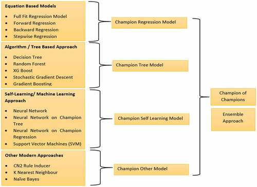
A ML framework is classified into four broad categories:

1. Equation based models—Full fit regression, forward regression, backward regression, stepwise regression

2. Algorithm/Tree based models—Decision tree misclassification, Decision tree probability, Random forest, Gradient boosting misclassification, Gradient boosting average square error

3. Machine Learning based models—Normal neural network, Neural network from champion regression, Neural network from champion tree

4. Other models—Memory based reasoning, Rule induction, Support vector machine

Analysis of the data will give us the best prediction model for each of the categories. This is termed as the “champion model” in the particular category. For example, four equation-based models run on a set of data may reveal that the forward regression model is providing the best prediction. This model will then be classified as the “champion model” in the “equation-based models” category. Similarly, the tree-based models applied on the same dataset may show that “decision tree probability approach” is providing the best prediction. This model will then be classified as the “champion model” in the “tree-based models” category.

As we can see, different approaches can come up with the best prediction models in the respective category, which we have termed as the “champion” model. But there needs to be “one” model—a “champion of champions” model that includes the best features of all the “champion” models’ from each category and thereby improve the prediction accuracy further. We term this as the “Ensemble Model”. The entire concept is presented in Figure 1.

Figure 1. The nomenclature for the proposed “ensemble model”.

5.2. Data collection

Data for the study was collected from published statistics of Government of Telangana, Government of India databases, and internet-enabled statistical data. Agricultural yield data for monthly production for all the districts for different crops were obtained from the open government data (OGD) platform India (https://data.gov.in/sector/agriculture?page=6). Soil statistics and irrigation statistics captured in the soil card was taken from Ministry of Statistics and Programme Implementation (http://mospi.nic.in). This was aggregated at the district level. Weather data was obtained from Directorate of Economics and Statistics, Government of Telangana (https://www.ecostat.telangana.gov.in/agricultural_statistics.html) and from the open portal of India Meteorological Department (2022) (https://mausam.imd.gov.in). Data on fertilizer consumption and fertilizer content in the soil at the district level was obtained from the portal of The Fertiliser Association of India (https://www.faidelhi.org/).

Monthly data was collected from 30 districts for 12 crops over a period of 10 years. This led us to 43,200 data points. After due cleansing of the data, suitable methodologies could be applied on 41,836 data points.

5.3. Data pre-processing

Once the 43,200 data points were accessed, the data pre-processing step was incorporated. This ensured that junk data is separated and the rest of the data points are standardized, normalized, and enhanced before further analysis. The data pre-processing included the following two steps.

1. Analyzing the data: The data is analysed using data profiling and then through data validation techniques explained below. The objective lies in focussing on the non-junk data for the next steps.

   • Data Profiling—This includes inspecting data for errors, inconsistencies, redundancies, and incomplete information. The objective lies in creating the data profiling reports to gauge the type of redundancies available in the data. Demographic variables are considered for data profiling. There were: Farmer Name, Farmer ID, Aadhar ID, Name of districts, villages, panchayats, etc. The analysis led to dropping of 878 observations where there was complete missing and junk values across the primary keys (Farmer Name, Farmer ID, and Aadhar ID). There were observations wherein one of the three variables (Farmer Name, Farmer ID and Aadhar ID) was present and the other information was validated and imputed by matching against the external sources (CBDT Income Tax Returns, E Parivahan, Beneficiary and Bank Details of the farmers from the Central Government and State Government schemes (Pradhan Mantri Krishi Sinchai Yojana—PMKSY, Pradhan Mantri Fasal Bima Yojana—PMFBY and Kisan Credit Card (KCC)).

   • Data Validation—This step involves separating junk and invalid datafrom the original dataset. Out of 43,200 data points, 878 observations are dropped, and 42,322 observations are considered to be valid for next steps.

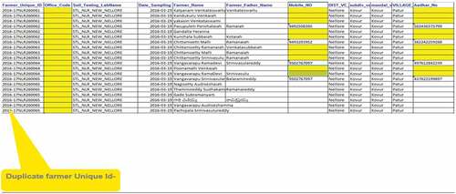
2. Improve the data quality: This step involves enhancing the data quality by incorporating deduplication (primary keys), outlier detection, data enrichment using imputation of missing values, and data capping at 99 percentile and 1 percentile values for the variables—yields, fertilizer statistics, farm statistics and weather statistics. The data quality and data enrichment methods are explained below.

   • Data Quality—This step includes deduplication of farmer demographics and farm demographics to remove duplicate rows. This step resulted in removal of 286 observations from the 42,322 observations taken from previous step. Annexures 1, 2 and 3 showcases few examples of the explained steps. The 42,036 observations are taken to the next step post deduplication.

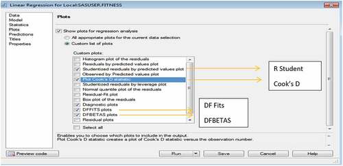
   • Data Enrichment—This step includes enhancing data and removing biases through outlier analysis and imputation. The outlier analysis using univariate analysis (box plot) and multivariate analysis (distance measures of Rstudent, Cook’s D, D F Fits and D F Betas) are incorporated on the different numeric factors like fertilizer statistics, farm statistics, weather conditions. Once these fourdistance metrics are incorporated, the common observations which are marked outliers by all the four methods are highlighted. The R student, Cook’s D and D F Fits zeroes in on the observations that are probable outliers; and the D F Betas focusses on the parameter across which a particular observation is being marked outlier. The common observations by the three methods (R student, Cook’s D and D F Fits) and the particular parameter against which the observation is marked outlier is taken from D F Betas. The next step involves checking against the parameter value (obtained from DF Betas) of the common observations from the three distance matrices and determining the percentile range where it exists. If the observation parameter value is more than 99 percentile value of the parameter, then the observation parameter is capped at 99 percentile. Similarly, if the observation parameter value is less than 1 percentile value of the parameter, then the observation parameter is capped at 1 percentile. The outlier detection techniques in SAS Enterprise Guide is presented in annexure 4. Of the 42,036 observations, there are 200 observations which had more than 25% of the parametric values missing. All these observations are rejected and 41,836 observations are taken for imputation. XG Boost algorithm is used to ensure that the estimated parameter values of the missing observations are best guess for the 41,836 observations. The parameter values for the different observations are normalized by using Z-score, ensuring that there is no biased impact in terms of coefficients of the different features evolving through biased observations during model development and model assessment.

5.4. Data analysis

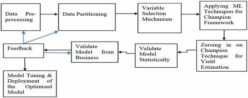
The procedure followed for data analysis on the 41,836 observations is provided inFigure 2.

Figure 2. Procedure followed for data analysis.

5.4.1. Target categorization and variable selection (statistical feature selection)

We categorise the yield of different crops as “high yield”, “medium yield” and “low yield”—based on the distribution analysis of the yield for each of the crops in a particular financial year for all the districts of Telangana. Total yield of a particular crop for all the districts in a financial year is defined as the total value of output of all the districts of the particular crop sown and harvested in a particular year. If a particular crop of particular districts in a particular financial year has a yield of more than 75 percentile value of the total yield, it is considered as “high yield”. If a particular crop of a particular districts in a particular financial year has a yield between 50 and 75 percentiles, it is considered as “medium yield” and if below 50 percentile, it is considered as “low yield”. Thus, “yield” becomes the target variable with three categorical classifications (high, medium, and low). The other parameters—weather variables, soil statistics, farmer statistics, irrigation statistics, and fertilizer statistics—become the independent variables.

5.4.2. Creation of modelling dataset (training, validation and cross validation)

The dataset is split into two halves—one is labelled as the training dataset and the other is the validation dataset. The training dataset is used to develop the ML models and the validation dataset is used to evaluate the model performance. The ratio of split of the data set for training and validation is 70:30. The number of observations used in the training dataset is 29,285 (70% of the 41,836 observations) and for validation dataset is 12,551 (30% of the 41,836 observations). Model assessment is done on the validation data (12,551 observations).

5.4.3. Variable selection mechanism and assessment criteria

The second step involves variable selection mechanism—selecting the significant variables from the superset of variables impacting the yield. The variable superset is shown in Table 2. The significant variables are selected from the training data using the statistical assessment criteria of Information Gain, Information Gain Ratio, Gini decrease, ANOVA, Chi Square, Relief F (Rank importance feature selection algorithm) and FCBF (Fast Correlation Based Filter for Feature Selection). The significant variables are highlighted in Table 2.These significant variables are used for model building as part of step 3.

Table 2. Independent variables used in the model

Variables/ dimensions	Different elements of the variables/ dimensions used in the model	Variables which evolved as statistically significant
Weather	Water level (gallons of water per square feet), humidity (average humidity in percentage), rainfall (average rainfall in mm), temperature (maximum temperature, minimum temperature, and average temperature-degree Celsius). The average maximum wind speed at the district (Max_WS_Avg).	The average maximum wind speed (Max_WS_Avg), Average rainfall and average temperature
Soil	Alluvial soil, black soil, loamy soil, red soil, acidic, alkaline, Amount of Boron content in the field (B_NA), Amount of chlorine content in the field (LT_CL), Whether the iodine content was more than the critical level (I Above Critical Level), Level of electrical conductivity in the seeds (EC_ Critical for germination), No of fields having the prevalence of red soil as soil characteristics in the district (ST_Red Soil)	Amount of Boron content in the field (B_NA), Amount of chlorine content in the field (LT_CL), Whether the iodine content was more than the critical level (I_Above Critical Level), Level of electrical conductivity in the seeds (EC_ Critical for germination), No of fields having the prevalence of red soil as soil characteristics in the district (ST_Red Soil)
Farmer	Number of farm labourers, number of farm owners, number of tenants, number of marginal farmers, number of small farmers., No of farms who cultivate a specific crop in the district (Farms_Cropwise), No of firms in the district having the prevalence of modern irrigation facilities including air pumps, etc. (IR_ Lift Irrigation)	No of farms who cultivate a specific crop in the district (Farms_Cropwise), No of firms in the district having the prevalence of modern irrigation facilities including air pumps, etc. (IR_ Lift Irrigation)
Irrigation	Type of irrigation for the field—Dry, Rainfed, Borewell, Canal, Tank, Open well, etc (IR_Irrigated)	Type of irrigation for the field—Dry, Rainfed, Borewell, Canal, Tank, Open well, etc (IR_Irrigated)
Fertiliser	Normal fertiliser, fertiliser injurious to crop, high-organic fertiliser, low-organic fertiliser, high potassium fertiliser, high nitrogen fertiliser. Amount of Propyne oxide contaminated in the field categorized into Low, Medium, and High based on the distribution (PO)	Amount of Propyne oxide contaminated in the field categorized into Low, Medium, and High based on the distribution (PO)

5.4.4. Applying ML techniques for champion framework

All the four broad categories of models as outlined in section 5.1, viz. Equation based models, Algorithm/Tree based models, Machine Learning based models and Other models are applied on the training dataset. The results presented in Table 3 illustrate the model performance carried out on the validation dataset. The best performing model is termed as the “champion model” for each category of models.

Table 3. Level 1 validation: model performance statistics for all the different models on the validation data

Category	Models	Measurement parameters
		ROC or AUC	Accuracy	Precision	Recall	F Score	Champion Model
Equation based models	Full fit regression	0.483	0.503	0.523	0.576	0.574	Forward regression
	Backward regression	0.492	0.517	0.516	0.504	0.502
	Forward regression	0.497	0.527	0.575	0.598	0.597
	Stepwise regression	0.467	0.502	0.517	0.557	0.562
Algorithm/ Tree Based Models	Decision Tree	0.914	0.907	0.907	0.907	0.907	Random Forest
	Random Forest	0.938	0.900	0.902	0.900	0.900
	XG Boost	0.860	0.860	0.863	0.860	0.860
	Stochastic Gradient Descent	0.933	0.933	0.938	0.933	0.933
	Gradient Boosting	0.500	0.923	0.852	0.923	0.886
Self-Learning / Machine Learning Based Models	Neural Network	0.487	0.517	0.565	0.588	0.587	Neural Network from Champion Tree
	Neural Network from Champion Regression	0.683	0.506	0.505	0.506	0.497
	Neural Network from Champion Tree	0.960	0.940	0.940	0.940	0.940
	Support Vector Machines (SVM)	0.955	0.900	0.900	0.900	0.900
Models based on other modern approaches	CN2 Rule Inducer (Learning Algorithm for Rule Induction)	0.923	0.887	0.887	0.887	0.887	CN2 Rule Inducer (Learning Algorithm for Rule Induction)
	K Nearest Neighbour (KNN)	0.727	0.673	0.675	0.673	0.673
	Naïve Bayes	0.850	0.908	0.909	0.908	0.908

5.4.5. Technology stack used

The data assessment and data validation including the data management activities (de duplication, standardization, normalization, imputation, and data quality report generation and data quality activities) is done using SAS Enterprise Guide and SAS DI Studio. The activities like feature selection, feature engineering, model development, model building, and model assessment is done using SAS Enterprise Guide. Few algorithms like XG Boost, SVM are called from Python and R libraries from the SAS Enterprise Miner using the SAS IML packages. The R Studio and the Orange interface was integrated on top of SAS Enterprise Miner using the SAS IML package for seamless and better user experience for the different business stakeholders (department officers, administrators, policy makers as well as IT and ML developers).

5.4.6. Model validation: Step 1: determining the champion model for yield estimation

Three levels of model validation for the different ML models are incorporated to ensure stable model performance and mitigating model biases.

At the first level of model validation (Level 1), the assessment of the different candidate ML models are done on the validation data of 12,551 observations (30% of the total data).The measurement parameters used for model validation and model performance testing for the first level are: Accuracy, Risk Operating Curve (ROC) or Area Under Curve (AUC), Precision, Recalland F Score (Harmonic Mean of Precision and Recall). A detailed description of these and also terminologies like sensitivity is available at https://towardsdatascience.com/accuracy-recall-precision-f-score-specificity-which-to-optimize-on-867d3f11124.The models that evolve as champions for each of the categories are showcased in Table 3 with the different model performance statistics. Higher AUC along with significant F value is the criteria for choosing of the champion model.

5.4.7. Model validation: Step 2: developing the optimized model—the “ensemble model”

As we can see, different approaches can come up with the best prediction models in the respective category, which we have termed as the “champion” model. But there needs to be “one” model—a “champion of champions” model that includes the best features of all the “champion” models and thereby improve the prediction accuracy further. We call this as the “Ensemble Model”. The Ensemble model aggregates the predicted probabilities of each observation for each of the individual models. Based on the predicted probability of each observation, the predicted target is calculated based on either of the three methods namely (a) averaging of the probabilities and then tagging the target based on the average probability, (b) taking the maximum probability of all the different models and tagging the target based on the maximum probability between the candidate models and (c) Voting method wherein for each of the of the different models, the individual target based on the individual probability is taken up for a particular observation and based on the voting method (the maximum classification of the observation for a particular target), the target is chosen.

All the above three methods for the ensemble model are applied on the training data 29,285 observations (70% of the total data) and validated on the validation data of 12,551 observations (30% of the total data). It emerged that the “Ensemble Model with Average Aggregation” wherein the ensemble node averages the predicted probabilities of all the candidate models is the best model with best performance.

The table below showcases the performance of the Ensemble Model with Average aggregation of the individual probabilities across the 5 assessment criteria being used for the other candidate models namely Accuracy, Risk Operating Curve (ROC) or Area Under Curve (AUC), Precision, Recall and F Score (Harmonic Mean of Precision and Recall) and has emerged as the best performance compared to the other candidate models.

The performance of the ensemble model above is assessed on the validation data.

5.4.8. Performance of the different combination of ensemble models on the validation data

There are three methods for aggregation of probabilities which are incorporated as part of the Ensemble model and are explained below.

(a) Averaging wherein the ensemble node averages the predicted probabilities of the preceding modeling nodes

(b) Maximum Probability wherein the maximum option sets the predicted probability as the highest predicted probability of all the trained models

(c) Voting Option of the predicted probability—the voting option for class variables has been done through (1) averaging the posterior probabilities of the most popular class and ignoring all other posterior probabilities (2) recalculate the posterior probability of each class by using the proportion of posterior probabilities that predict that class.

We have used all the three options for our ensemble model. Table 4 highlights Performance of ensemble model (average aggregation of individual probabilities). Table 5 showcases the performance of the different aggregation methods and the best performing Ensemble model. It emerged that the “Ensemble Model with Average Aggregation” wherein the ensemble node averages the predicted probabilities of the preceding modelling nodes emerged as the best model with best performance. The criteria remain the same—the method with highest AUC and a significant F score. We term this as the “champion of champions” model.

Table 4. Performance of ensemble model (average aggregation of individual probabilities)

Category	Aggregation function of the probabilities used for Ensembling	Measurement parameters
		ROC or AUC	Accuracy	Precision	Recall	F Score	Champion model
Ensemble Model	Averaging	0.985	0.953	0.955	0.953	0.953	Ensemble model with the average aggregation

Table 5. Performance of different ensemble models on the validation data

Category	Aggregation function of the probabilities used for Ensembling	Measurement parameters
		ROC or AUC	Accuracy	Precision	Recall	F Score	Champion Model
Ensemble Model	Averaging	0.985	0.953	0.955	0.953	0.953	Ensemble Model with Average Aggregation
	Maximum Probability	0.959	0.869	0.866	0.869	0.867
	Voting Option (Averaging the posterior probabilities of the most popular class)	0.932	0.852	0.855	0.857	0.861
	Voting Option (Recalculate the posterior probability of each class by using the proportion of posterior probabilities that predict that class)	0.912	0.849	0.852	0.849	0.852

Of all the different combination of ensemble model being used, the averaging of the individual probabilities from the different models emerged as the champion model as showcased above. The different combinations of ensemble model used are:

(a) averaging of the probabilities and then tagging the target based on the average probability

(b) taking the maximum probability of all the different models and tagging the target based on the maximum probability between the candidate models and

(c) Voting method wherein for each of the of the different models, the individual target based on the individual probability is taken up for a particular observation and based on the voting method (the maximum classification of the observation for a particular target), the target is chosen.

Post the calculation of the average probability for the Ensemble model, the threshold for the cut off is taken to be 0.5. Any average probability value of ≥0.5 (average of all the probabilities of individual models) will place a value in that particular target. The justification of the 0.5 cut off can be incorporated from Table 6 wherein the cut off at 0.5 showcases the maximum value of the sum of the specificity and sensitivity for the ensemble model.

Table 6. Optimized cut-off for the ensemble model

Cut Off	Sensitivity	Specificity	Sum
0.01	69.70	100	169.70
0.10	90.60	93.20	183.80
0.20	92.30	93.20	185.50
0.30	93.10	93.60	186.70
0.40	94.10	94.30	188.40
0.50	95.30	95.50	190.80
0.60	95.30	76.50	171.80
0.70	92.30	76.50	168.80
0.80	87.80	75.30	163.10
0.90	100	33.30	133.30
0.99	100	0	100.00

A snapshot of the results as obtained from SAS Enterprise Miner and Python is presented in Figure 3.

Figure 3. Snapshot of results obtained.

5.4.9. Further model validation of the Ensemble Model (average probability aggregation)

The model performance is gauged using Lift and Cumulative Ratio on the validation data for testing stable performance post the assessment criteria in the above step as a second level of validation.

The Lift of a model is a measure of how much better one can expect to do with the predictive model comparing without a model. It is the ratio of gain % to the random expectation % at a given decile level. The Lift ratio on the validation data is used to gauge the performance of the predictive model compared to a no model.

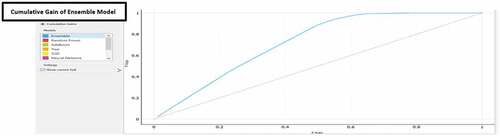
The cumulative gains curve is an evaluation curve that assesses the performance of the model and compares the results with the random pick. It shows the percentage of targets reached when considering a certain percentage of the population with the highest probability to be target according to the model.

The Lift of the Ensemble is showcased in Table 7 as well as in Figure 4 where in the ensemble model has a consistent lift across the different deciles.

Figure 4. Lift curve analysis of the ensemble model (average probability aggregation).

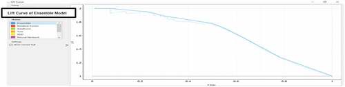
Table 7. Lift analysis of ensemble model (average probability aggregation): 2nd level of model validation

Decile	Lift	Interpretation
10	2	The Ensemble model is able to classify twice the events (High Yield, Medium Yield and Low Yield) compared to a no model or a baseline model.
20	1.90	The Ensemble model is able to classify 1.9 times the events (High Yield, Medium Yield and Low Yield) compared to a no model or a baseline model.
40	1.86	The Ensemble model is able to classify 1.86 times the events (High Yield, Medium Yield and Low Yield) compared to a no model or a baseline model.
60	1.64	The Ensemble model is able to classify 1.64 times the events (High Yield, Medium Yield and Low Yield) compared to a no model or a baseline model.
80	1.36	The Ensemble model is able to classify 1.36 times the events (High Yield, Medium Yield and Low Yield) compared to a no model or a baseline model.

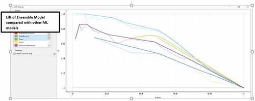
Table 8 showcases the Cumulative gain analysis of ensemble model - 2nd level of model validation. The Lift of the Ensemble model compared with the other candidate models in the validation data is also showcased in Figure 5 wherein it has a significant more lift (marked in blue) across the different deciles compared with the other candidate ML algorithms.

Table 8. Cumulative gain analysis of ensemble model: 2nd level of model validation

Decile	Cumulative gain	Interpretation
20	0.40	By targeting top 20% of the observations in the validation data based on the predicted probability (Category—High Yield) we will be able to focus on 40% of the high yield cases.
40	0.70	By targeting top 40% of the observations in the validation data based on the predicted probability (Category—High Yield) we will be able to focus on 70% of the high yield cases.
60	0.95	By targeting top 60% of the observations in the validation data based on the predicted probability (Category—High Yield) we will be able to focus on 95 % of the high yield cases.

Figure 5. Lift curve analysis of the ensemble model (average probability aggregation) compared with other ML models.

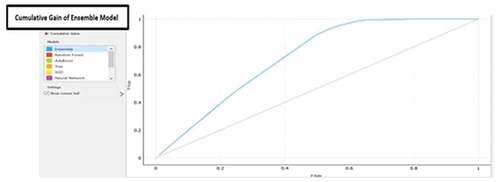
The Cumulative Gain of the Ensemble model is showcased in table 9 below as well as in Figure 6 below wherein the ensemble model has a consistent cumulative gain across the different deciles. By focussing on the top 40% of the observations having highest predicted probability of High Yield, 70% of the total cases of high yield being captured. Similarly, by focussing on top 60% of the observations having highest predicted probability of high yield, 95% of the total cases of high yield being captured. Both the statistics showcase strong model performance of the Ensemble model.

Figure 6. Cumulative gain analysis of the ensemble model.

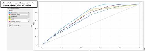
The Cumulative Gain of the Ensemble model compared with the other candidate models in the validation data is also showcased below in Figure 7 wherein it has a significant more lift (marked in blue) across the different deciles compared with the other candidate ML algorithms.

Figure 7. Cumulative gain analysis of the ensemble model compared with other ML models: 2nd level of model validation.

5.4.10. Stress testing using cross validation method: level 3 of model validation

To ensure that the model performance is not impacted by overfitting, a third level of independent model validation and stress testing is conducted. The objective here is to ascertain the model performance of the champion model (Ensemble Approach) against the candidate other ML techniques. The approach incorporated for this validation method is 10-fold cross validation. The total data points (both training and validation) of 41,836 observations are divided into 10 folds or segments. Thus, each segment or fold comprises of approximately 4183 observations. The different ML models are built on 9 such fold (37,647 observations) and is stress tested or validated on the other 1-fold (4189 observations). The last fold had six more observations than 4183 because of random sampling and approximation methods. This process is continued for 10 iterations wherein the 9 folds are used for model building and 1-fold for model validation. The model validation technique includes average of all the assessment parameters like Accuracy, Risk Operating Curve (ROC) or Area Under Curve (AUC), Precision, Recall and F Score (Harmonic Mean of Precision and Recall) across 10 iterations (41,890 observations across 10 iterations). The average model performance for the mentioned five parameters—accuracy, risk operating curve (ROC) or area under curve (AUC), precision, recall and F score (harmonic mean of precision and recall) across 10 iterations for the different ML models is showcased in Figure 8.

Figure 8. 10-fold model cross validation: 3^rd level of model validation.

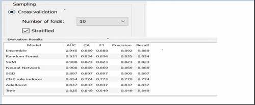
The 10-fold cross validation output for the Ensemble Model in Figure 9 above has strong AUC, classification, F1 score, Precision and Recall values compared to other ML models showcasing optimized model performance removing any over fitting bias.

Figure 9. Cumulative Gain of Ensemble Model

5.4.11. Validate model from business

The champion model is again validated from the subject matter experts from the state and central government officials at Telangana Agricultural Ministry. The subject matter experts gave their feedback on the appropriateness of the features selected for the model. This was done to ensure that there is an alignment and validation from stakeholders across for easy adoption of data driven decision making for yield estimation.

5.4.12. Feedback

A feedback loop has been incorporated that has a provision for testing a hypothesis, adding a new feature and check the prediction accuracy and tweaking. This would help in continuous monitoring of the model validity post the solution is deployed and also help in more proactive adoption by the users.

6. Conclusion and implication for future research

This study uses modern ML and AI techniques for estimating crop yield using different data elements including weather, soil, farmers, irrigation and fertiliser to predict the supply side of crop production. The study becomes more relevant in a setting with varied demographies and different methods of data collection and aggregation. The proposed ensemble methodology has not been applied and reported in academic literature. Future lies in taking the supply side yield estimation as an input to match the demand of the market and incorporate price forecasts. The accurate yield estimation and the resulting optimized price forecasts in line with the demand would ensure significant increase of farmer income thus enhancing the value chain of all the stakeholders in the entire agriculture eco system. There is also a significant scope of using the ensemble ML approach in predicting the yield estimates on other data samples and extending the framework of analysis.

Disclosure statement

No potential conflict of interest was reported by the authors.

Additional information

Funding

The authors received no direct funding for this research

Annexure 1: Deduplication of duplicate farmer unique ID

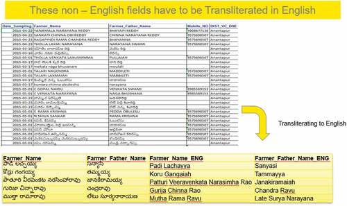
Annexure 2: Data Translation to English for the analysis using standard tools

Annexure 3: Data validation of the Aadhar No: Data Quality Activities

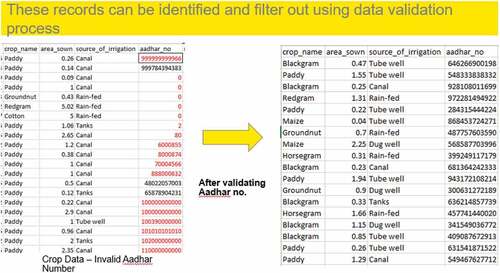
Annexure 4: Outlier Detection Techniques using different distance algorithms: SAS Enterprise Guide

References

- (2021). Retrieved January 15, 2022, from GOV/Agriculture: https://data.gov.in/sector/agriculture?page=6
- (2022). Retrieved February 26, 2022, from Ecostat/Telengana/Agriculture: https://www.ecostat.telangana.gov.in/agricultural_statistics.html
- Aleminew, A., Tadesse, T., Merene, Y., Bayu, W., & Dessalegn, Y. (2020). Effect of integrated technologies on the productivity of maize, sorghum and pearl millet crops for improving resilience capacity to climate change effects in the dry lands of Eastern Amhara, Ethiopia. Cogent Food & Agriculture, 6. https://doi.org/10.1080/23311932.2020.1728084
- Bakar, K. S., & Jin, H. (2020). Areal prediction of survey data using bayesian spatial generalised linear models. Communications in Statistics: Simulation and Computation, 49(11), 2963–21 https://doi.org/10.1080/03610918.2018.1530787.
- Balaji, P., & Dakshayinib, M. (2018). Performance analysis of the regression and time series predictive models using parallel implementation for agricultural data. Procedia Computer Science, 132, 198–207. https://doi.org/10.1016/j.procs.2018.05.187
- Beulah, R. (2019). A survey on different data mining techniques for crop yield prediction. International Journal of Computer Science Engineering, 7 1 , 738–743 https://www.ijcseonline.org/pdf_paper_view.php?paper_id=3576&.
- Chen, Y., Song, H.-S., Yang, Y.-N., & wang, G.-F. (2021). Fault detection in mixture production process based on wavelet packet and support vector machine. Journal of Intelligent & Fuzzy Systems, 40(5), 10235–201803. https://doi.org/10.3233/JIFS-201803
- The Fertiliser association of India (2022). Retrieved 03 2022, from https://www.faidelhi.org/https://towardsdatascience.com/accuracy-recall-precision-f-score-specificity-which-to-optimize-on-867d3f11124
- Galguera, L., Luna, D., & Méndez, M. P. (2006). Predictive segmentation in action: Using CHAID to segment loyalty card holders. International Journal of Market Research, 48(4), 459–479. https://doi.org/10.1177/147078530604800407
- Gandhi, & Armstrong, (2016). A review of the application of data mining techniques for decision making in agriculture. Proceedings of the 2016 2nd international conference on contemporary computing andInformatics. 1–6. https://doi.org/10.1109/IC3I.2016.7917925
- GOVERNMENT OF INDIA, MINISTRY OF STATISTICS AND PROGRAMME IMPLEMENTATION. (2021). Retrieved February 21, 2022, from https://mospi.gov.in/documents/213904/416359//CPI%20Press%20Release%20November%2020211639397393459.pdf/c65bf379-9db6-fd28-4f04-fcd70a17726a
- INDIAN METEOROLOGICAL DEPARTMENT. (2022). Retrieved 01 02, 2022, from https://mausam.imd.gov.in/
- Loh, W.-Y. (2011, February). Classification and regression trees, WIRES data mining and knowledge discovery. 14–23. John Wiley & Sons Inc. https://doi.org/10.1002/widm.8
- Mishra, P. S., & Mishra, B. N. (2015). Machine learning techniques in plant biology. In Plant omics: the omics of plant science (pp. 731–754). Springer India.https://doi.org/10.1007/978-81-322-2172-2_26
- Mrinalini, K., Vijayalakshmi, P., & Nagarajan, T. (2021). Feature‐weighted AdaBoost classifier for punctuation prediction in Tamil and Hindi NLP systems. Expert Systems 39(3) , 1–19. https://doi.org/10.1111/exsy.12889
- Priya, M. (2018). Role of image processing and machine learning techniques in disease recognition, diagnosis, and yield prediction of crops: A review. International Journal of Advanced Research in Computer Science, 9(2), 788–795 http://www.ijarcs.info/index.php/Ijarcs/article/view/5793.
- Ramalingam, S., & Baskaran, K. (2021). An efficient data prediction model using hybrid harris hawk optimization with random forest algorithm in wireless sensor network. Journal of Intelligent & Fuzzy Systems, 40(3), 5171–201921. https://doi.org/10.3233/JIFS-201921
- Sellam, V., & Poovammal, E. (2016). Prediction of crop yield using regression analysis. Indian Journal of Science and Technology, 9(38), 1–5. https://doi.org/10.17485/ijst/2016/v9i38/91714
- Sengupta, R. (2020). DownToEarth. Retrieved 05 November 2022, from https://www.downtoearth.org.in/news/agriculture/every-day-28-people-dependent-on-farming-die-by-suicide-in-india-73194
- Singh, N., Singh, P., Thampi Sabu, M., El-Alfy, E.-S. M., Thampi, S. M., & El-Alfy, E. S. M. (2019). A novel bagged naïve bayes-decision tree approach for multi-class classification problems. Journal of Intelligent & Fuzzy Systems.Vol, 36(3), 2261–2271. https://doi.org/10.3233/JIFS-169937
- Tarekegn, K., Asado, A., Gafaro, T., & Shitaye, Y. (2020). Value chain analysis of banana in bench maji and sheka zones of southern Ethiopia. Cogent Food &agriculture, 6(1), 1785103. https://doi.org/10.1080/23311932.2020.1785103
- Thomas van Klompenburg, Ayalew Kassahun, Cagatay Catal. et al (2020). Crop yield prediction using machine learning: A systematic literature review. Computer and Electronics in Agriculture, 177, 105709. https://doi.org/10.1016/j.compag.2020.105709 https://www.sciencedirect.com/science/article/pii/S0168169920302301. ISSN 0168-1699
- Trizoglou, P., Liu, X., & Lin, Z. (2021). Fault detection by an ensemble framework of Extreme Gradient Boosting (XGBoost) in the operation of offshore wind turbines. An International Journal, 179(C), 945–962. https://doi.org/10.1016/j.renene.2021.07.085
- Xanthopoulos, P., Pardalos, P. M., & Trafalis, T. B. (2013). linear discriminant analysis. In Robust data mining. springer briefs in optimization (pp. NY. 27–33). Springer. https://doi.org/10.1007/978-1-4419-9878-14