Agriculture growth in Ghana: A time-series analysis with autoregressive distributed lag approach

Abstract

The lack of empirical research on the effect of financial development and interest rate on agricultural growth hinders effective policy orientation towards poverty reduction. This paper is set to examine the effect of financial development and interest on agricultural growth from the Ghanaian perspective. We used time-series data for the period 1980–2020. The time-series autoregressive distributed lag approach was used to investigate the relationship between the underlying variables. The cumulative sum chart and cumulative sum of squares statistics were used to show that our model is stable and does not contain any serious structural change. The results show that financial development and interest rates have a significantly positive effect on agricultural growth in both the long-run and short-run. The results also suggest that the government should pay more attention to both short-term and long-term policies to enhance agricultural growth through improving macroeconomic variables like reducing interest rate and enhancing accessibility to agricultural financial services in the country. We propose that agribusinesses be encouraged by enacting new financial reforms to stimulate agri-based commercial ventures, particularly in the agricultural sector. We further suggest that in order to boost agricultural growth in the country, the government should focus on lowering the prices of agri-based inputs such as seeds, fertilizers, and fuel, as well as encouraging research and development efforts. By analyzing the effect of financial development and interest rate on agricultural growth, this paper contributes to evidence-based explanations for the need to implement policies that will boost agricultural production and, hence, poverty reduction.

Keywords:

• financial development
• interest rates
• agricultural growth
• autoregressive distributed lag
• Ghana

1. Introduction

Agriculture is the backbone sector of the economies of developing countries and continues to assist several African nations in surviving and thriving (Ariom et al., 2022; Gusev & Koshkina, 2022). The agriculture sector employs around 70% of Africa’s workforce and despite this, Africa’s agricultural development falls behind that of other continents (Bouët et al., 2022; Daum et al., 2022; Suri & Udry, 2022). Concern about sustainable agricultural growth is a pressing issue of development (Serova, 2022). This requires knowledge of the dynamics driving the agricultural growth in Ghana.

Agriculture plays a crucial part in Ghana’s economy, contributing to employment, foreign exchange, government income, food security, the provision of raw materials for agro-processing enterprises, the growth of industrial product markets, and its ties to other sectors (Hossin, 2020). This is consistent with the economic literature, which emphasizes the importance of agriculture to economic development (Ahmed et al., 2020; Islam, 2020; Kamenya et al., 2022). Due to the significance of the sector to the economy, its success “all things being equal” influences the overall economic performance (Tahir et al., 2019). As a consequence, if agricultural production increases greatly, the gross domestic product (GDP) of the whole economy increases proportionally, and vice versa, everything else being equal. Consequently, rapid agricultural production will greatly contribute to Ghana’s industrialization and economic growth.

By examining the numerous connections between agricultural growth and financial markets, for instance, Ngong et al. (2022), Farooq et al. (2021) and Nejad et al. (2018), demonstrate the financial sector’s strength as a stimulant for agricultural growth and, consequently, economic growth. The question that needs to be answered explicitly is whether nations with a developed finance sector use agricultural resources more effectively, and what is the nature of long-run and short-run relationship between agricultural growth, financial development, and interest rate?

There is evidence that little thought has been given to the prospect of a financial sector development transmission mechanism that increases national agricultural productivity, especially in developing countries and Ghana in particular. From existing studies, it is noted that the impact and direction of the productivity-financial development nexus remain mostly unclear (Boltianska et al., 2021; Khanal & Omobitan, 2020). Understanding this link and likely endogeneity at the national level is essential for designing policies and initiatives to enhance the financial sector while supporting greater agricultural development within an economy.

Over the years, the agriculture sector had the lowest performance in the Ghanaian economy (Setsoafia et al., 2022). It is therefore vital to know the factors that drive growth in the Ghanaian agricultural sector in order to enact policies that promote poverty reduction and structural change.

In emerging nations such as Ghana, the dynamic link between interest rate fluctuations, financial growth, and agricultural expansion has not been well examined. Madsen et al. (2021) argues that the link between financial development and growth should be unidirectional, with financial development driving to growth. As a result, the study adopted the time series autoregressive distributive lag (ARDL) model to provide a foundation for analysing the short-term and long-term relationship between financial development and interest rates, and possible impact on agricultural growth in Ghana. This paper contributes to existing studies and offers new insights into the effects of financial development and interest rate on the agricultural productivity in Ghana. Since a large proportion of the Ghanaian population is engaged in agricultural activities.

2. Literature review

The theoretical concept that underpins this current study and hence the productivity growth is the neoclassical and analytical model pioneered by Solow (1956). This model establishes a series of equations showing the relationship between labour-time, capital goods, output, and investment. This model assumes that countries use their resources efficiently and that there are constant returns to scale, diminishing marginal productivity of capital, exogenously determined technical progress, and substitutability between capital and labour (Okafor & Shaibu, 2016). According to this view, the role of technological change is very important.

A major challenge with growth modelling is the determination of the variables to be included in the analysis, which has led to different variables that have been proposed as potential growth determinants. For instance, some studies (Agyemang et al., 2022; Mwangi, 2021; Tsaurai, 2022) recently have explored the factors underlying agricultural growth. These studies have placed emphasis on different kinds of explanatory variables and offered various insights into the sources of agricultural growth. This issue results because of the open-endedness of growth theories whereby the validity of one causal theory does not imply the falsity of another (Okafor & Shaibu, 2016).

Various studies have analysed the effect of different explanatory variables on agricultural productivity or performance. For instance, some studies focus on access to finance (Chandio et al., 2022; Guo et al., 2022), credit supply (Seven & Tumen, 2020), credit constraints (Shuaibu & Nchake, 2021) and agricultural productivity. Some other studies focus on how financial development affects agricultural productivity.

Increased access to capital expands the investment options available to farmers and improves their risk management and product development capabilities. Multiple studies have shown a link between economic growth and agricultural expansion (Oluwole et al., 2021; Raihan & Tuspekova, 2022).

High interest rates, which invariably leads to high credit costs, have the potential to affect agricultural growth. Hossin (2020) studied the link between interest rate fluctuations, financial development, and agricultural growth in Bangladesh using an annual time-series dataset from 1980 to 2014 to examine the causal link between financial development and economic growth and it was demonstrated that the link between deposit rates and economic growth is bidirectional. He also indicates that a deregulated deposit rate of interest will raise financial depth and eventually enhance the economic growth of Bangladesh.

Ochalibe et al. (2019) using data from 1980 to 2018 examined the effect of interest rate policy tools on Nigeria’s agricultural growth and establishes that the link between interest rates and agricultural growth is unidirectional.

There are limited studies conducted on the determinants of agricultural growth in Ghana. Even the few existing studies from the Ghanaian perspective (Akudugu, 2016; Danso-Abbeam et al., 2018; Sekyi et al., 2021) have also considered different explanatory parameters as factors that influence agricultural productivity.

For instance, Tetteh et al. (2022) in a recent study analysed the effects of climate change variables on agricultural production in Ghana. The results reveal that temperature is inimical to overall food production and maize and roots and tubers production, while precipitation is good for cereal and maize production.

Again, in a recent study, Frimpong et al. (2022) carried out a study to identify agricultural development in Ghana as well as try to identify challenges of modern agricultural development in Ghana. It was found that access to financial support is a major hindrance to agricultural productivity in Ghana. In a related study, Bambio et al. (2022) assess the effects of increased exposure to agricultural technologies on agricultural productivity, hence farmers’ economic well-being in Ghana and some neighbouring countries like Mali and Senegal using post-implementation data collected in 2019. Danso-Abbeam et al. (2018) have identified the critical role of extension programmes as the main factors influencing agricultural productivity in the northern part of Ghana. Again, Enu and Attah-Obeng (2013) considered, real exchange rate, labour force, and real GDP per capita as the main variables, influencing agricultural production in Ghana. A similar study in Ghana by Tsiboe et al. (2021) also argue that growth in agricultural productivity is determined by other factors such as subsidy on fertilizer and agricultural credit.

3. Methods and material

This analysis utilizes Ghana’s yearly time-series data spanning 41 years (from 1980 to 2020). Agricultural growth, physical capital, labour, government expenditures, and trade openness were all calculated as a percentage of GDP, while financial development and interest rates were measured as an index and yearly rates, respectively.

3.1. Model specification

Let us consider the traditional growth model with two inputs with the assumption of constant returns to scale as:

(1) $Y_i=A{K_t}^{\alpha }{L_t}^{\beta }{e}^{u_t}$(1)

where Y is agricultural productivity, K represents capital and L stands for labour. The parameters α and ß are marginal impacts of capital and labour on agricultural productivity, and they lie between 0 and 1, i.e. 0 < α < 1and 0 < ß < 1. t refers to time period, and µ is stochastic error term.

The production function in equation (1)(1) $Y_i=A{K_t}^{\alpha }{L_t}^{\beta }{e}^{u_t}$(1) has the capacity to include more factors of production. Financial development, trade openness, government spending, labour, and interest rates are all economic factors that may influence agricultural growth.

Given that we incorporate financial development (F) and interest rate in the model, then equation (1)(1) $Y_i=A{K_t}^{\alpha }{L_t}^{\beta }{e}^{u_t}$(1) becomes:

(2) $Y_t=A{K_t}^{\alpha }{L}_t^{\beta }{F}_t^{\gamma }{I}_t^{\delta }{e}^{{\mu }_t}$(2)

Where the new parameters $\gamma$ and $\delta$must lie between 0 and 1, i.e. $0<\gamma <1$ and $0<\delta <1$and these show the marginal impact of financial development and interest rate on agricultural productivity, respectively.

In order to establish the linearity relationship between the dependent and independent variables, we take natural logarithm of equation (2)(2) $Y_t=A{K_t}^{\alpha }{L}_t^{\beta }{F}_t^{\gamma }{I}_t^{\delta }{e}^{{\mu }_t}$(2) , the above equation becomes:

(3) $y_t={\beta }_0+\alpha k_t+\beta l_t+\gamma f_t+\delta I+{\mu }_t$(3)

There are other factors that also affect agriculture growth such as trade openness, government spending, and physical capital. Therefore, equation (3)(3) $y_t={\beta }_0+\alpha k_t+\beta l_t+\gamma f_t+\delta I+{\mu }_t$(3) in its augmented form can be specified as follows:

(4) $A{G}_t={\beta }_0+{\beta }_{1}F{D}_t+{\beta }_{2}I{R}_t+{\beta }_{3}P{C}_t+{\beta }_{4}L{C}_t+{\beta }_{5}G{E}_t+{\beta }_{6}T{O}_t+e_t$(4)

In the model, that is equation (4)(4) $A{G}_t={\beta }_0+{\beta }_{1}F{D}_t+{\beta }_{2}I{R}_t+{\beta }_{3}P{C}_t+{\beta }_{4}L{C}_t+{\beta }_{5}G{E}_t+{\beta }_{6}T{O}_t+e_t$(4) the agriculture growth (AG), which is agriculture’s contribution to GDP is used as the dependent variable for analyzing the impact. According to Fonseca and Van Doornik (2022), financial development (FD) refers to the rise in the quantity, quality, and effectiveness of intermediary financial services, and this is a key explanatory variable within the model. Financial development seeks to enhance the efficacy of allocating financial resources and monitoring capital projects by promoting competition and improving the status of the financial system.

The lending interest rate (IR) is a bank rate that typically suits the private sector’s short and medium-term borrowing demands. This rate is constantly altered depending on the creditworthiness of the borrowers and their financing goals. The lower the interest rate on loans in Ghana, the greater the number of farmers who would be able to receive money to expand production. In this research, the loan interest rate is employed as a proxy for farmer access to financing. This is another key explanatory variable included in our model.

In this study, the amount of physical capital (PC) was proxied by the proportion of real gross domestic investment to GDP. Quality capital is essential to the agricultural development of any country since it tends to spur expansion. Increased capital expenditure has a direct effect on a nation's GDP. This is due to the fact that greater capital accumulation via investment necessitates an increase in capital per worker, which necessitates technological progress and the development of the requisite skills and training to successfully use new capital inputs. As a consequence, the growth rate would accelerate.

The quantity and caliber of a country’s labour force (LC) are crucial determinants of its future development model. The labour force is the complete labour stock or currently active population of all individuals who met the requirements for work or unemployment during a certain time period (Azar et al., 2022). According to the traditional growth model, agricultural expansion and the stock of productive labour in any economy are positively correlated, hence it is anticipated that the coefficient, will be positive.

Government expenditure (GE) on agriculture refers to the amount of money spent by the government on the agricultural sector for development. The variable is proxied by the government’s monetary supply to the agricultural sector. Trade openness (TO) establishes country’s trade activities with the outside world and this has the potential to influence growth and agricultural productivity. The trade openness is calculated by dividing the total of exports and imports by GDP. Exports of goods and services represent the total value of all commodities and other market services provided to the rest of the world. Furthermore, imports of goods and services represent the total value of all commodities, and other market services received from the rest of the world. As a result, the trade openness coefficient is expected to be positive.

3.2. Estimation technique

We adopt the ARDL approach to address our objectives. The ARDL is a dynamic estimation method that produces efficient estimates even when the variables of the study exhibit different orders of integrations such as zero (0) and one (1). As such, the ARDL cointegration technique is preferable when dealing with variables that are integrated of different order, I(0), I(1), or combination of the both, and robust when there is a single long-run relationship between the underlying variables in a small sample size. The long-run relationship between the underlying variables is detected through the F-statistic (Wald test). Also, the effect of an adjustment in the agriculture growth to a change in financial development, interest rates, and other explanatory variables of interest may take time and not instantaneous, and the ARDL approach, in this case, is suitable for such a model.

4. Unit root tests

In other to to achieve the reliability of stationarity test, both the Phillips-Perron (PP) and ADF tests were employed. The PP which is nonparametric test is a generalization of the ADF that accepts less rigorous assumptions about time-series. Contrary to the alternative (stationary), the null hypothesis asserts that the variable under examination has unit roots (is non-stationary). The ADF’s fundamental formulation is as follows:

(5) $Y_t=\mu +\alpha Y_{t-1}+{\gamma }_t+{\epsilon }_t$(5)

Subtraction of ${\mathrm{Y}}_{\mathrm{t}-1}$ from both sides of equation (5) yields:

(6) $\mathrm{\Delta }{Y}_t=\mu +\left(\alpha -1\right)Y_{t-1}+{\gamma }_t+{\epsilon }_t$(6)

Now, set (α-1) to be equal to ρ gives equation (5) below:

(7) $\mathrm{\Delta }{Y}_t=\mu +\rho Y_{t-1}+{\gamma }_t+{\epsilon }_t$(7)

Allowing (α-1) to be equal to ρ and adjusting for serial correlation by adding lagged first differenced to equation (7) yields the ADF test of the form:

(8) $\mathrm{\Delta }{Y}_t=\mu +\rho Y_t+{\gamma }_t+\sum _{i=1}^{\rho }{\beta }_i\mathrm{\Delta }{Y}_{t-1}+{\epsilon }_t$(8)

Where $Y$ is the time series at time $t$, $\mathrm{\Delta }$ is the difference operator, $\mu$, $\gamma$ and ${\beta }_t$are the parameters to be estimated, and ${\epsilon }_t$is the stochastic random disturbance term.

The ADF and PP compare the null hypothesis that a series contains unit roots (non-stationary) to the alternative hypothesis that there are no unit roots (stationary). These are written as:

_H0: ρ = 0 (Y_t is non-stationary)

_H1: ρ<0 (Yt is stationary)

If the rho statistic is less negative than the critical values, the null hypothesis is not rejected, and we conclude that the series is non-stationary. If the tau value or t-statistic is more negative than the critical values, the null hypothesis is rejected, and the series is concluded to be stationary. ARDL’s ECM version was used to calculate the rate of adjustment to equilibrium.

The following constrained (conditional) version of the ARDL model is estimated to evaluate the long-run relationship between the variables of interest in order to carry out the limits test process for cointegration which is denoted as:

(9) $\begin{array}{rl}& \mathrm{\Delta }A{G}_t={\beta }_0+\theta G{E}_{t-1}+{\beta }_{1}F{D}_{t-1}+{\beta }_{1}F{D}_{t-1}+{\beta }_{2}I{R}_{t-1}+{\beta }_{3}L{B}_{t-1}+{\beta }_{5}G{E}_{t-1}\\ & +{\beta }_{6}T{O}_{t-1}+\sum _{i=0}^{\rho }\phi A{G}_{t-i}+\sum _{i=0}^{\rho }{\gamma }_{1i}F{D}_{t-i}+\sum _{i=0}^{\rho }{\gamma }_{2i}I{R}_{t-i}+\sum _{i=0}^{\rho }{\gamma }_{3i}P{C}_{t-i}\\ & +\sum _{i=0}^{\rho }{\gamma }_{4i}L{B}_{t-i}+\sum _{i=0}^{\rho }{\gamma }_{5i}G{E}_{t-i}+\sum _{i=0}^{\rho }{\gamma }_{6i}T{O}_{t-i}\end{array}$(9)

Where Δ is the first difference operator, ρ is the lag order choosen by the Schwarz Bayesian Criterion (SBC), the parameters $\theta$ and ${\beta }_{\mathrm{i}}$ denote the long run parameters and $\phi$ and ${\gamma }_{\mathrm{j}\mathrm{i}}$ are the short-run parameters of the model to be estimated through the error correction framework in the ARDL model, ${\beta }_0$ is the constant term (drift), while ${\mu }_{\mathrm{t}}$ is a white noise error term which is N(0,${\delta }^2$).

The null hypothesis, that there is no long-run relationship between the variables in equation (9), is compared to the alternative hypothesis, that there is a long-run relationship between the variables. The hypothesis tested is specified as:

$H_0:{\beta }_i=0$against $H_1:{\beta }_i\ne 0;$for $i=1,2,\cdots 6.$

Pesaran et al. (2001) generated and presented the appropriate critical values based on the number of independent variables in the model of the presence or absence of a constant term or time trend, given that the asymptotic distribution of F-statistics is non-standard without considering the independent variables being I(0) or I(1) (1).

5. Long-run and short-run dynamics

After establishing cointegration from the ARDL model, the next step is to estimate the following $\mathrm{A}\mathrm{R}\mathrm{D}\mathrm{L}\left(\mathrm{P},\hspace{0.17em}{\mathrm{q}}^1,{\mathrm{q}}^2,{\mathrm{q}}^3,{\mathrm{q}}^4,{\mathrm{q}}^5,{\mathrm{q}}^6\right)$ model to obtain the long-run coefficients.

(10) $\begin{array}{rl}& \mathrm{\Delta }A{G}_t={\vartheta }_0+\sum _{i=0}^{\rho }{\tau }_{1}A{G}_{t-i}+\sum _{i=0}^{q^1}{\tau }_{2}F{D}_{t-i}+\sum _{i=0}^{q^2}{\tau }_{3}I{R}_{t-i}+\sum _{i=0}^{q^3}{\tau }_{4}P{C}_{t-i}\\ & +\sum _{i=0}^{q^4}{\tau }_{5}L{B}_{t-i}+\sum _{i=0}^{q^5}{\tau }_{6}G{E}_{t-i}+\sum _{i=0}^{q^6}{\tau }_{7}T{O}_{t-i}+{\epsilon }_t\end{array}$(10)

Equation (10) is then used to estimate the variables’ short-run parameters using the ARDL model’s error correction representation. ARDL’s error correction version is used to calculate the speed of adjustment to equilibrium. When the variables have a long-term relationship, the unrestricted ARDL error correction representation is roughly as follows:

(11) $\begin{array}{rl}& \mathrm{\Delta }A{G}_t={\theta }_0+\sum _{i=0}^p{\lambda }_{1i}A{G}_{t-i}+\sum _{i=0}^{q^1}{\lambda }_{2i}F{D}_{t-i}+\sum _{i=0}^{q^2}{\lambda }_{3i}I{R}_{t-i}+\sum _{i=0}^{q^3}{\lambda }_{4i}P{C}_{t-i}+\sum _{i=0}^{q^4}{\lambda }_{5i}L{B}_{t-i}\\ & +\sum _{i=0}^{q^5}{\lambda }_{6i}G{E}_{t-i}+\sum _{i=0}^{q^6}{\lambda }_{2i}T{O}_{t-i}+\upsilon EC{T}_{t-1}+{\epsilon }_t\end{array}$(11)

Where the coefficients represent the short-run dynamics, $E{C}_{t-1}$ is the error-correction term or residuals derived from the equation, and is the rate of adjustment to long-run equilibrium following a shock to the system (10). The cointegration equation residuals with a one-period lag can be written as follows:

(12) $\begin{array}{rl}& ECT=A{G}_t-{\theta }_0-\sum _{i=0}^p{\lambda }_{1i}A{G}_{t-1}-\sum _{i=0}^{q^1}{\lambda }_{2i}F{D}_{t-i}-\sum _{i=0}^{q^2}{\lambda }_{3i}I{R}_{t-i}\\ & -\sum _{i=0}^{q^3}{\lambda }_{4i}P{C}_{t-i}-\sum _{i=0}^{q^4}{\lambda }_{5i}L{B}_{t-i}-\sum _{i=0}^{q^5}{\lambda }_{6i}G{E}_{t-i}-\sum _{i=0}^{q^6}{\lambda }_{7i}T{O}_{t-i}\end{array}$(12)

The error correction term in the dynamic model indicates the rate of adjustment to long-run equilibrium. In other words, the magnitude indicates how quickly the variables recover from perturbation. It is statistically significant if it has a negative sign. Any short-term shock will be compensated for in the long run, according to the negative sign. The higher the coefficient of the error correction factor, the faster the convergence to equilibrium. Diagnostic and stability tests are also carried out to validate the goodness of fit of the model.

5.1. Stability test

To verify the stability of the estimated coefficients of the model, the Cumulative Sum of Square (CUSUMSQ) and Cumulative Sum (CUSUM) were used. For a stable model, the CUSUMSQ statistic line is expected to fall within the lower and upper bounds at a significance level of 5% (Tule et al., 2018). This also applies to the CUSUM.

The diagnostic test examines the serial correlation, functional form, normalcy, and heteroscedasticity of the chosen model. Conducting stability tests are critical, according to Pesaran and Pesaran (1997). If the plots of CUSUM and CUSUMSQ statistics remain within the 5% level of significance, the null hypothesis of stable coefficients in the provided regression cannot be rejected.

(13) $A{G}_t={\vartheta }_0+{\displaystyle \sum _{i=0}^p{\tau }_{1}F{D}_{t-i}}+{\displaystyle \sum _{i=0}^n{\tau }_2\Delta \ln I{R}_{t-i}}+{\displaystyle \sum _{i=0}^n{\tau }_3\Delta \ln GE{X}_{t-i}}+{\displaystyle \sum _{i=0}^n{\tau }_4\Delta \ln HC{E}_{t-i}}+{\displaystyle \sum _{i=0}^n{\tau }_5\Delta \ln AG{R}_{t-i}}+{\displaystyle \sum _{i=0}^n{\tau }_6\Delta \ln MA{N}_{t-i}}+{\displaystyle \sum _{i=0}^n{\tau }_7\Delta \ln SE{R}_{t-i}}+{\displaystyle \sum _{i=0}^n{\tau }_8\Delta \ln EX{P}_{t-i}}+\lambda EC{M}_{t-i}$(13)

6. Test for Granger causality

Following the identification of economically relevant cointegrating vectors, the research investigates causality by regressing each variable on lagged values of itself and the other. To determine the direction of causation between Y and X, the Granger causality test was used. The following are the specifications:

(14) $\mathrm{\Delta }{Y}_t={\gamma }_0+\sum _{i=1}^n\varphi Y_{t-1}+\sum _{i=1}^m\varpi \mathrm{\Delta }{X}_{t-1}+{\upsilon }_t$(14)

(15) $\mathrm{\Delta }{X}_t={\pi }_0+\sum _{j=1}^m{\eta }_i{X}_{t-1}+\sum _{i=1}^n{\psi }_i\mathrm{\Delta }{Y}_{t-1}+{\nu }_t$(15)

Where ${\upsilon }_t$and ${\nu }_t$ are mutually uncorrelated white noise error terms such that ΔY and ΔX are the non-stationary dependents, and independent variables, while n and m are the optimal lag order.

7. Results and discussion

Table 1 provides the statistical properties of all of the study’s data. The mean and variances were employed to measure the central trends, while the standard deviation was used to account for the dispersion of the variables around the mean.

Table 1. Descriptive statistics

	AG	FD	IR	GE	LB	PC	TO
Mean	36.484	0.106	49.881	9.848	49.733	1.841	63.111
Median	36.484	0.103	24.477	9.708	49.733	1.973	69.357
Maximum	59.730	0.147	241.378	15.308	57.120	11.315	116.048
Minimum	17.306	0.063	0.081	5.861	29.750	−9.542	6.320
Std. Dev.	11.746	0.019	63.262	2.300	7.456	3.590	27.728
Skewness	0.114	0.405	1.495	0.425	−1.461	−.867	−0.332
Kurtosis	2.162	2.873	4.473	2.506	4.198	5.846	2.499
Jarque-Bera	1.286	1.150	18.988	1.652	17.040	18.986	1.183
Probability	0.525	0.563	7.5x10^−3	0.438	1.9x10^−4	7.5x10−5	0.553

Table 1 shows that time-series data covering 41 years was used for this investigation, with all variables having positive values (means). For example, the average agricultural growth (AG) was 36.48. This suggests that agricultural growth is about 36.48% on average over the study period. In the same period, financial development averaged approximately 0.106. This suggests that financial development contributes for around 0.11% across the research period.

The agricultural interest rate also averaged 49.88, indicating that the agricultural sector lending rate accounts for about 49.88% over the study period The mean of Government expenditure on Agriculture averaged around 9.847. This shows that about 9.85% of government expenditure is on agriculture over the study period. Labour (LB) representing employment in Agriculture also recorded a mean of 49.733, which implies that labour needed for agriculture accounts for 49.73% of Total labour over the study period.

Physical capital consisting of infrastructure and technology in agriculture averaged 1.84. This shows that on the average investment in agriculture in terms of equipment and technology is 1.84% over the study period. Finally, trade openness, on the other hand, averaged around 63.11 with a Jarque–Bera value of 1.183. This implies that on averagely, total trade to international market accounts for 63.11%. Again, the kurtosis of the variables, with values ranging from 2.16 to 5.84, reveals that they are normally skewed.

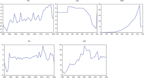
A unit root test was conducted prior to utilizing the ARDL approach for cointegration, and the Granger causality test to determine the stationarity of the data. As a consequence, all variables were studied by examining their trends graphically, plots of time-series help determine whether or not the trend is stationary. From Figure 1, it could be observed that almost all variables are non-stationary in terms of their respective levels.

Figure 1. Graphical trends of the variables.

The Augmented Dickey–Fuller (ADF) and Phillips–Perron (PP) tests were used to precisely determine the order of integration in levels and the first difference for all variables.

Table 2 displays the results of the ADF and PP tests for unit root with intercept and trend in the model for all variables. In accordance with the null hypothesis, the series is neither stationary nor has a unit root. MacKinnon, critical values, and probability values are used to reject the null hypothesis for the test.

Table 2. Unit root test results: ADF and PP test

Variable		ADF		PP
		Intercept	Int & Trend	Intercept	Int & Trend
AG	I(0)	−1.945	−2.456	−1.921	−2.048
	I(1)	−4.198***	−4.248***	−3.152**	−2.848
FD	I(0)	−2.364	−3.412*	−2.221	−3.364*
	I(1)	−7.132***	−7.123***	−8.556***	−9.121***
INTR	I(0)	−0.965	1.189	−1.729	−2.528
	I(1)	3.048*	−3.025*	−6.337***	−6279***
GEX	I(0)	−2.959**	−2.981	−3.079**	−3.099
	I(1)	−6.477***	−6.414***	−8.184***	−12.167***
LAB	I(0)	−2.548	−2.829	−2.679	−2.942
	I(1)	−4.144**	−4.567**	−5.144**	−5.567**
PC	I(0)	−3.178**	−3.424*	−2.882*	−3.009
	I(1)	−6.902***	−6.927***	−8.366***	−13.706***
TOP	I(0)	−1.809	−1.557	−1.814	−1.557
	I(1)	−5.912***	−6.382***	−6.142***	−6.451***

Note: ***, **, and * indicate the rejection of the non-stationary null hypothesis at the 1%, 5%, and 10% level of significance.

Based on the unit root test results in Table 2, the null hypothesis of the absence of unit root in the variables at their levels can be rejected only for GE (government expenditure) and PC (physical capital), because the P-values of the ADF statistic of government expenditure and physical capital are statistically significant at 5%. This means that at levels where the variables are integrated to order zero, government spending and physical capital are stationary I(0).

However, because the P-values of the ADF statistics for these variables are not statistically significant at any of the three traditional levels of significance, the null hypothesis of the existence of a unit root cannot be rejected at levels. Nonetheless, when the variables that were not stationary at initial levels were compared, they all became stationary at the 5% and 1% levels of significance. As a result, because all first differenced estimates have statistically significant P-values of the ADF statistic at the 5% and 1% levels, the null hypothesis of the existence of a unit root (non-stationary) is rejected.

The PP test was also used to determine whether the variables were stationary. Table 2 also includes the results of the PP test for unit root with intercept and trend at levels, as well as the first difference in the model for all variables.

Table 2 shows that the variables are non-stationary at levels because P-values of PP statistics are not statistically significant at any of the conventional levels of significance, with the exception of government expenditure, physical capital, and financial development at 5% and 10%, respectively. Because the P-values of the PP statistics for these variables are statistically significant at 10% and 1% significance levels, the null hypothesis of the presence of unit root in the variables at their levels can be rejected only for government expenditure, financial development, and physical capital. This implies that government spending, financial development, and physical capital are all at a standstill, implying that the variables are integrated with order zero I(0).

However, after the first difference all of the variables become stationary. This is because the null hypothesis of the existence of a unit root (non-stationary) is rejected at 10, 5, and 1% significant levels for all variables. The series is a combination of integrated variable of order zero I(0) and order one I(1), according to the ADF test, the PP test for unit roots (1). Since the test results demonstrated the absence of I(2) variables, the estimate is now performed using the ARDL method. The following sections discuss the cointegration findings, long-run and short-run results, and Granger causality test results.

With the null hypothesis of no long-run linkages between the predictor and outcome variables, the bound testing technique was used to specify the presence of cointegration among the dependent and explanatory variables. The test’s F-statistics validated the combined importance of all explanatory factors on the dependent variable. As a result, it is clear whether or not the coefficients of the various variables are equal to zero. The findings are summarised in Table 3.

Table 3. Results of bounds test for existence of cointegration

F-Bounds Test		Null Hypothesis: No levels relationship
Test Statistic	Value	Signif.	I(0)	I(1)
F-statistic	4.081569	10%	1.99	2.94
K	6	5%	2.27	3.28
		2.5%	2.55	3.61
		1%	2.88	3.99

The Schwarz Bayesian Criterion was used to pick the ARDL model (1, 1, 2, 2, 2, 2, 2). When agricultural growth (AG) is used as the dependent variable, the 1% significance level rejects the joint null hypothesis of lagged level variables (that is, addition test) of the coefficients being zero (no cointegration). At the 1% significance level, the calculated F-statistic is 4.0816, more significant than the upper limit critical value of 3.99. This implies that agricultural growth and its explanatory factors have a long-run relationship, thereby rejecting the null hypothesis of no cointegration among the variables.

These findings imply that there is a distinct cointegration relationship between agricultural expansion and the explanatory variable. After establishing the presence of a long-run link between agricultural growth and its explanatory factors, the long-run and short-run estimates of the ARDL models in equations (10) and (11) were calculated to obtain the long-run and short-run coefficients and standard errors.

Based on the findings of the cointegration analysis, the long-run relationship among the variables was approximated using the ARDL framework, and the results are shown in Table 4. Because it produces parsimonious results, the Akaike Information Criterion (AIC) was used to estimate the long-run ARDL model. Given the yearly nature of the data collection, estimation was performed with a two-year lag.

Table 4. Estimation of long run results

Dependent Variable: AG ARDL (1, 2, 2, 0, 2, 2, 2)
Variable	Coefficient	Std. Error	t-Statistic	Prob.
FD	4.994348	1.248462	4.000401	0.0006***
INTR	−0.082032	0.045106	−1.818640	0.0833*
GE	0.234767	0.493353	0.475860	0.6391
LB	1.588502	0.388366	4.090222	0.0005***
PC	1.434219	0.420290	3.412451	0.0026***
TO	0.012435	0.056532	0.219967	0.8280
C	140.0493	24.31685	5.759352	0.0000

Note: *** and * denotes significance level at 1% and 10% respectively.

As shown in Table 4, the coefficient of financial development measured by the financial development index is positive and statistically significant at the 1% level of significance, which is consistent with the first objective of examining the effect of financial development on agricultural growth. This shows that if Ghana’s financial development advances by one-unit, agricultural growth will increase by 4.99%. This implies that, throughout the research period, increased financial sector development has the potential to boost agricultural sector growth in Ghana. It could be argued that as the financial sector grows, credit becomes more accessible to the private sector, resulting in more agricultural investment and an increase in the agricultural sector’s rate of development. This finding also lends support to the study’s alternative hypothesis. Financial development has a significant beneficial effect on agricultural growth, according to Hossin (2020) and Setsoafia et al. (2022) financial development has a significant beneficial effect.

The impact of interest rates on agricultural expansion is also considered. Table 4 shows that interest rates have a detrimental impact on agricultural development in Ghana. As a result, an increase in the interest rate of 0.08% would limit agricultural growth. This means that when interest rates rise, financing becomes more costly for the private sector, reducing investment in agriculture and lowering the agricultural sector’s growth rate. This data also supports the study’s alternate hypothesis that interest rates significantly impact agricultural development in Ghana. This research backs up the results of Ochalibe et al. (2019), Kamenya et al. (2022), and Islam (2020), who discovered that interest rates have a considerable impact on an economy’s agricultural development.

The coefficient of labour proxied by agricultural sector employment (ages 15 to 64 years) was found to be positive, confirming the prior expectation and statistically significant at the 1% significance level. This means that every additional unit of population (ages 15–64) increases agricultural growth by 1.59%. Intuitively, more human resources predict higher levels of productivity, and because agricultural growth is positively related to labour supply, an increase in labour supply improves long-term growth outcomes. This is consistent with the findings of Ochalibe et al. (2019) who discovered that the labour force has a positive influence on agricultural development. As a result, labour is determined to be a factor in Ghana’s agricultural expansion.

Finally, the long-run relationship between the physical capital coefficient and the trade balance is positive and statistically significant, validating the a-prior expectation and statistically significant at the 1% significance level. This means that an increase in agricultural investment of 1% results in an increase in agricultural growth of 1.43% in the economy. This means that increased agricultural investment leads to the purchase of more equipment and machinery. This assistance increases agricultural output by boosting agricultural production. The findings support those of Ngong et al. (2022), Nejad et al. (2018) who discovered that physical capital had a positive impact on agricultural development. As a result, physical capital is said to be a significant factor in Ghana’s agricultural development.

According to economic intuition, the error correction model (ECT-1) measures the rate at which an endogenous variable adapts to shocks in an explanatory variable in order to converge to its long run equilibrium. Table 5 shows that the predicted ECT-1 coefficient is negative and statistically significant at the one percent error level. The ECT-1 coefficient is negative and significant, confirming the cointegration findings. Following a short-run shock, the ECT-1 measures how far financial development, interest rates, government spending, labour, physical capital, and trade openness have recovered to long-run equilibrium. The outcome of a short run shock reveals a high rate of convergence to the long run equilibrium per year. In other words, after any short-term shock, equilibrium shifts by approximately 52.57% per year in the long run.

Table 5. Estimates of short-run results of error correction model

Variable	Coefficient	Std. Error	t-Statistic	Prob.
D(FD)	1.001064	0.341818	2.928649	.0080***
D(FD(−1))	1.102367	0.315816	3.490539	.0022***
D(INTR)	−0.002926	0.009759	−0.299782	.7673
D(INTR(−1))	0.067610	0.015346	4.405656	.0002***
D(LAB)	0.783969	0.144978	5.407515	.0000***
D(LAB(−1))	−0.761294	0.205711	−3.700798	.0013***
D(PC)	0.482177	0.102149	4.720316	.0001***
D(PC(−1))	−0.395230	0.122589	−3.224037	.0041***
D(TOP)	0.013178	0.028313	−0.465446	.6464
D(TOP(−1))	−0.069191	0.029320	−2.359850	.028**
CointEq(−1)*	−0.525709	0.079674	−6.598237	.000***
R-squared	0.928953	Mean dependent var		0.216554
Adjusted R-squared	0.903578	S.D. dependent var		5.975376
S.E. of regression	1.855463	Akaike info criterion		4.306891
Sum squared resid	96.39684	Schwarz criterion		4.776101
Log likelihood	−72.98438	Hannan-Quinn criter.		4.475240
Durbin-Watson stat	2.089814

Note: ***, ** denotes significance level at 1% and 5%, respectively.

The short-run coefficient of financial development is positive and statistically significant, according to the findings. This corresponds to the long-term outcomes discussed in the preceding section. A unit increase in financial development leads to a 1.001% increase in agricultural growth in the short run at a 1% significance level. However, in the short run, the “lagged” coefficient of financial development improves agricultural growth in the country. A one-unit increase in the “lagged” financial development variable causes a 1.102% increase in Ghana’s agricultural output in the short run. Hossin (2020) confirm similar findings.

Furthermore, the findings indicate that the “lagged” interest rate coefficient causes a short-term improvement in the country's agriculture. A one-unit increase in the “lagged” interest rate variable leads to a 6.7% improvement in Ghana’s agricultural output in the short-run. El-Rasoul and Morsi (2020) and Kamenya et al. (2022) recently confirmed similar findings. Also, the findings show that the short-run labour coefficient is positive and statistically significant. This corresponds to the long-term outcomes discussed in the preceding section. A unit increase in labour leads to a 0.78% increase in agricultural growth in the short run at a 1% significance level.

However, in the short run, the “lagged” coefficient of labour reduces agricultural growth in the country. A one-unit increase in the “lagged” labour variable reduces Ghana’s agricultural growth by 0.76% in the short run. Furthermore, the results show that the short-run physical capital coefficient is positive and statistically significant. This corresponds to the long-term outcomes discussed in the preceding section. A unit increase in physical capital leads to a 0.48% increase in agricultural growth in the short run at a 1% significance level. However, in the short run, the “lagged” coefficient of physical capital reduces agricultural growth in the country. A unit increase in the “lagged” physical capital variable reduces Ghana’s economic growth by 0.395% in the short run. The findings agreed with those of Chandio et al. (2022) and Khanal and Omobitan (2020).

The findings indicate that the “lagged” coefficient of trade openness reduces agricultural output in the short run. A one-unit increase in the “lagged” trade openness variable reduces Ghana’s agricultural growth by 0.069 in the short run. The findings agreed with those of Tahir et al. (2019).

The potency of this ARDL model was verified on the following assumptions (i.e., null hypothesis): 1) There is no serial correlation, 2) there is no heteroskedasticity (or ARCH effect), 3) the residual follows the normal distribution, 4) the model is not incorrectly specified, and 5) the long run model is not unstable. Table 6 displays the results of the potency test.

Table 6. Residual diagnostic test

Test Statistics	F Version	LM Version
A. Normality	N/A	CHSQ(2) = 0.7876*** [0.477]
B. Serial Correlation	F(3,21) = 1.9059***[0.1596]	CHSQ(1) = 8.132*** [0.1434]
C. Heteroscedasticity	F(14,23) = 0.5669***[0.8635]	CHSQ(1) = 9.7471*** [0.7804]
D. Functional Form	F(1,23) = 0.0449***[0.8341]	CHSQ(1) = 0.2118*** [0.8341]

Note: *** We fail to reject the Null hypothesis at a 5% level of significance.

A: Based on a test of Skewness and kurtosis of residualsB: Lagrange multiplier test of residual serial correlationC: Based on the regression of squared residuals on squared fitted valuesD: Ramsey’s RESET test using the square of the fitted values

The table depicts clearly that the ARDL model contains no autocorrelation (i.e., the covariance of the error term is equal to zero) and no heteroskedasticity (i.e. constant variance of the error term). Again, the residuals follow the normal distribution, and the model is correctly specified. This is because we fail to reject the null hypothesis. After all, the probability values under each test are greater than 5%, demonstrating that the model has no such flaw. Hence, the model is potent at a 5% allowable error level.

The CUSUM and CUSUMSQ plots are shown in Figures 2 and 3, respectively.

Figure 2. CUSUM Plot.

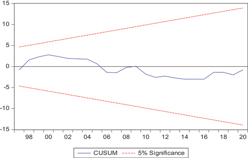
Figure 3. CUSUMSQ Plot.

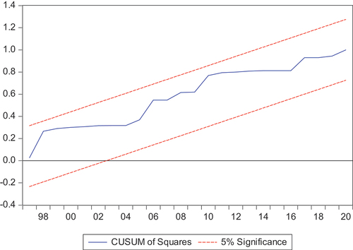
Figure 2 depicts the CUSUM plot for, the calculated ARDL model. The null hypothesis states that the coefficient vector remains constant over time, while the alternative hypothesis states that it does not. The CUSUM data are presented in relation to a 5% significance level critical limit. If the plot of these statistics stays within the critical limit of 5% significance level, the null hypothesis that all coefficients are stable cannot be rejected. Figure 2 shows no evidence of coefficient instability because all coefficient plots remain within the critical boundaries at the 5% significance level. As a result, the coefficients of the calculated model remain constant throughout the investigation. Figure 3 depicts the CUSUMSQ plot for, the estimated ARDL model. All coefficient plots fall below the critical boundaries at the 5% significance level, indicating that the coefficients are not unstable. As a result, the coefficients of the calculated model remain constant throughout the investigation. Finally, the CUSUM and CUSUMSQ tests show that the agricultural growth coefficients and explanatory variables in the model are stable.

Table 7 displays the results of the Granger causality test. The pairwise Granger causality test was used to determine the nature of the causal relationship between macroeconomic variables, confirming the cointegration analysis results and assisting in policy direction.

Table 7. Results of the pairwise Granger causality tests

Null Hypothesis:	Obs	F-Statistic	Prob.
FD does not Granger Cause AG	38	7.77691	0.0721*
AG does not Granger Cause FD		1.87948	0.1536
INTR does not Granger Cause AG	38	22.5039	0.0061***
AG does not Granger Cause INTR		0.99860	0.4065
GEX does not Granger Cause AG	38	1.90932	0.1486
AG does not Granger Cause GEX		0.50116	0.6842
LAB does not Granger Cause AG	38	3.21398	0.0363**
AG does not Granger Cause LAB		0.45988	0.7123
PC does not Granger Cause AG	38	0.01389	0.9977
AG does not Granger Cause PC		0.68261	0.5694
TOP does not Granger Cause AG	38	0.11859	0.9485
AG does not Granger Cause TOP		2.02076	0.1314

Note: ***, **, * denote rejection of null hypothesis at 1%, 5%, and 10% significance level.

The Granger causality test results in Table 7 shows that at a 1% significance level, the null hypothesis that financial development does not Granger cause agricultural growth is rejected. This means that Granger’s financial development causes agricultural growth. However, the null hypothesis that agricultural growth does not cause financial development is not rejected, implying that agricultural growth does not cause financial development, implying unidirectional causality between financial development and agricultural growth. This finding suggests that data from Ghana support the finance-led growth hypothesis. The findings are consistent with the bound test and with the findings of Hossin (2020) who obtained similar results.

Similarly, the study indicates that the null hypothesis that interest rates do not cause agricultural growth is not rejected. However, at a 1% significance level, the null hypothesis that agricultural growth does not Granger cause interest rates is rejected. This means that interest rates influence agricultural growth. This suggests that the relationship between interest rates and agricultural growth is unidirectional.

At a 5% level of significance, further analysis of the results rejected the null hypothesis that labour supply does not cause agricultural growth. The null hypothesis that real GDP does not Granger cause labour supply, on the other hand, is not rejected, implying that labour lag values do not predict variations in agricultural growth. As a result, there is one-way causality from labour to agricultural growth.

Finally, the rejection of both the null hypothesis that agricultural growth does not Granger cause physical capital, government expenditure, and trade openness, as well as the converse hypothesis, implies that there is no direction of causality between agricultural growth, physical capital, government expenditure, and trade openness over the study period.

Table 8 depicts the VDF of the variables in equation 6 over a 10-year period using an estimated VAR model and provides a sense of dynamics. A cursory glance at the data in Table 8 reveals that the projected error variance of agricultural growth within the 10-year horizon is the product of its own shock.

Table 8. Variance decomposition results

Period	S.E.	AG	FD	INTR	GEX	LAB	PC	TOP
1	3.316	100.000	0.000	0.000	0.000	0.000	.000	.000
2	4.181	63.268	3.219	0.003	0.364	32.956	.138	.049
3	6.452	26.563	1.703	43.946	1.983	25.234	.280	.287
4	6.818	31.477	2.484	39.691	2.331	22.623	.317	1.075
5	7.488	26.106	4.648	42.718	2.001	21.675	1.567	1.283
6	7.859	25.858	4.220	40.017	2.351	24.124	1.835	1.592
7	8.011	26.614	4.190	40.108	2.331	23.222	1.996	1.536
8	8.960	21.554	3.571	49.388	2.445	19.463	2.052	1.523
9	9.163	21.410	3.415	47.478	2.374	21.596	1.994	1.732
10	9.257	22.202	3.365	46.799	2.731	21.161	1.955	1.785

It can be inferred from Table 8 that a complete shock in agricultural growth results from innovation in the agricultural growth itself in the first quarter. In the second quarter, the major contribution of variation in the agricultural growth is by itself (63.26%) and labour 32.95%.

Interest rates and labour were the major contributors to variation in agricultural growth from the third to the fifth quarter. From the sixth quarter to the tenth quarter, interest rate contributed most to the agricultural growth with 40.02%, 40.11%, 49.38%, 47.47%, and 46.79% variations, respectively. Also, labour contributes more to the agricultural growth as the next after interest rate with 24.12%, 23.22%, 19.46%, 21.59%, and 21.16% variations, respectively.

Financial development, physical capital, government expenditure, and trade openness also had some innovations but were minimal.

These results confirm the findings of Ahmed et al. (2020) and Azar et al. (2022) that interest rate and labour significantly impact the agricultural growth of an economy.

Plots of the generalised impulse response functions of agricultural growth concerning financial development, interest rate, government spending, labour, physical capital, and trade openness are shown in Figure 4. This method depicts the reaction of one variable to an unexpected shock in another variable over a specific time period, providing insight into the variables’ dynamic connections. Each graph shows the number of quarters after the impulse has been initiated on the horizontal axis and the responses of the corresponding variable on the vertical axis.

Figure 4. Impulse response results.

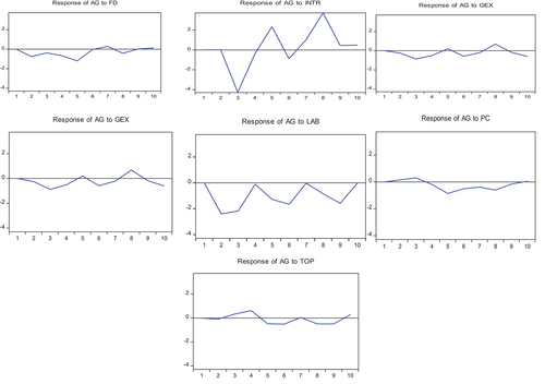
Figure 4 illustrates a pairwise simulation of the behaviour of the macroeconomic variables under consideration. It can be observed that the agricultural growth experienced some form of depreciation for the first 5 years and had some stability thereafter. However, the agricultural growth was stable for the first two years and dropped sharply in the third year, afterward a steady rise to the sixth year and fluctuated afterward in Figure 4.

A shock in government expenditure resulted in a moderate fluctuating trend in agricultural growth from the first year to the eighth-year forecast. Subsequent years saw the decreasing rate in agricultural growth at a relatively better rate, as shown in Figure 4. A general fluctuating in labour when predicted on an impulse in agricultural growth is also presented in Figure 4 Again, the agricultural growth witnessed an appreciation in year one but made a somewhat depreciable fall in value after being subjected to a physical capital in year 3 and afterwards, an unstable fluctuation persists. Figure 4 further shows that the respective annual movements of trade openness emanating from a shock in agricultural growth.

8. Conclusion and policy recommendation

The objective of this paper was to examine the effect of financial development and interest rate on agricultural growth from the Ghanaian perspective. We used annual time-series data for the period 1980–2020. The ARDL model is the empirical methodology we used in our analyses.

By modifying the traditional growth function, we established the common link between financial development, interest rates, and agricultural production. Increasing Ghana’s financial growth may be an advantageous in both the short and long-term. Rising interest rates, on the other hand, may not always benefit the agricultural sector because only the lag of interest rates had a significant (positive) influence on agricultural output levels in the short run. Aside from labour and physical capital, which had a significant impact on agricultural output in both the long and short run, none of the other control variables had a significant impact on agricultural output. The ARDL model’s diagnostic tests revealed no serial correlation, missing variables, or heteroscedasticity. The model parameters computed are structurally stable, with normal residuals.

A Granger causality test was performed to support the study’s objectives. Financial development, interest rates, labour, and physical capital all have a unidirectional Granger causal influence on agricultural production, according to research. This validates the ARDL regression results and supports the prior expectations. The impulse response function and variance decomposition were also employed in order to further investigation of the variables.

While financial development has a positive impact on agricultural growth, our findings suggest that the government should prioritise agriculture to improve productivity by improving rural population access to financial resources at a lower cost in order to capitalise on agriculture and increase the sector’s contribution to overall economic growth. New financial reforms, particularly for the agricultural sector, should be put in place to stimulate agribusiness ventures. The government should prioritise lowering the prices of agricultural inputs such as seeds, fertilisers, electricity, oil, and fuel, as well as encouraging research and development efforts to increase agricultural productivity. This would increase agriculture’s GDP contribution as well as the growth of other sectors such as industry and services. It is also necessary to develop the most critical road infrastructure connecting rural communities to agricultural markets.

By analysing the effect of financial development and interest on agricultural growth, this paper contributes to evidence-based explanations for the need to function out policies that will boost agricultural production and hence poverty reduction.

Our study has some limitations within which our findings need to be interpreted carefully. First, the research presented here was restricted to Ghana. However, the variables used in this study are major economic variables that affect the agricultural sector of almost all developing and under-developed economies. There may also be other variables that may impact on agriculture development apart from those we considered in our study.

Disclosure statement

No potential conflict of interest was reported by the authors.

Additional information

Funding

This research did not receive any specific grant from funding agencies in the public, commercial, or not-for-profit sectors.

Notes on contributors

Albert Ayi Ashiagbor

Albert Ayi Ashiagbor is a certified quantitative risk management and data analytic consultant. He is currently a Lecturer at the University of Professional Studies, Accra, where he teaches various courses such as Business Statistics, Quantitative Methods, Actuarial Science, Pension Management, Data and Machine learning, Actuarial Risk Management, Actuarial Finance and Research Methods in Pensions at both undergraduate and graduate levels. Ayi holds his PhD in Applied Statistics from the University for Development Studies. Prior to that, he had his Master of Philosophy (MPhil) in Statistics and also MPhil in Risk Management and Insurance both from University of Ghana. Ayi also holds Master of Education (M.Ed) degree in Educational Management and Practice from the Methodist University and University of Education, Winneba, Ghana. Ayi has experience in both academic and industrial research. He specializes in data analytic, statistical distributions, time series models, machine learning, generalized linear models, visualization, risk management and statistical computing.

Sylvia Ablateye

Sylvia Ablateye has received her MPhil in Finance from the University of Professional Studies, Accra. Currently, she is a full-time lecturer and administrator at Knutford University, Ghana. She has keen research interests on issues of agriculture financing, agriculture productivity, climate change and variability, time series, as well as environment and natural resource management.

Kojo Amonkwandoh Essel-Mensah

Kojo Amonkwandoh Essel-Mensah qualified as a Fellow of the Institute and Faculty of Actuaries (UK) in 2012. He is currently a Fellow member of both the Actuarial Society of South Africa and Actuarial Society of Ghana. He holds a PhD in Actuarial Science from the University of Pretoria, South Africa, an MSc (with distinction) in Mathematical Statistics from Rhodes University in South Africa and a BSc (Hons) in Mathematics and Statistics from the University of Ghana. Kojo is currently a Director and Senior Actuary of Berrybright Limited. He is also a Senior Lecturer in Actuarial Science at University of Professional Studies, Accra. Kojo has over twenty years’ experience in the Financial Sector and over ten years’ experience in Academia. Kojo’s financial sector experience is mainly in the Life Insurance Industry.

References

- Agyemang, S. A., Ratinger, T., & Bavorová, M. (2022). The impact of agricultural input subsidy on productivity: The case of Ghana. European Journal of Development Research, 34(3), 1460–20. https://doi.org/10.1057/s41287-021-00430-z
- Ahmed, F., Hossain, M. J., & Tareque, M. (2020). Investigating the roles of physical infrastructure, financial development and human capital on economic growth in Bangladesh. Journal of Infrastructure Development, 12(2), 154–175. https://doi.org/10.1177/0974930620961479
- Akudugu, M. A. (2016). Agricultural productivity, credit and farm size nexus in Africa: A case study of Ghana. Agricultural Finance Review, 76(2), 288–308. https://doi.org/10.1108/AFR-12-2015-0058
- Ariom, T. O., Dimon, E., Nambeye, E., Diouf, N. S., Adelusi, O. O., & Boudalia, S. (2022). Climate-smart agriculture in African countries: A review of strategies and impacts on smallholder farmers. Sustainability, 14(18), 11370. https://doi.org/10.3390/su141811370
- Azar, J., Marinescu, I., & Steinbaum, M. (2022). Labor market concentration. Journal of Human Resources, 57(S), S167–S199. https://doi.org/10.3368/jhr.monopsony.1218-9914R1
- Bambio, Y., Deb, A., & Kazianga, H. (2022). Exposure to agricultural technologies and adoption: The West Africa agricultural productivity program in Ghana, Senegal and Mali. Food Policy, 113, 102288. https://doi.org/10.1016/j.foodpol.2022.102288
- Boltianska, N. I., Manita, I. Y., & Komar, A. S. (2021). Justification of the energy saving mechanism in the agricultural sector. 1(19), 7–12. https://doi.org/10.5281/zenodo.6828908
- Bouët, A., Odjo, S. P., & Zaki, C. (2022). Africa agriculture trade monitor 2022Vol. 2022. Intl Food Policy Res Inst. https://doi.org/10.54067/9781737916437
- Chandio, A. A., Jiang, Y., Abbas, Q., Amin, A., & Mohsin, M. (2022). Does financial development enhance agricultural production in the long‐run? Evidence from China. Journal of Public Affairs, 22(2), e2342. https://doi.org/10.1002/pa.2486
- Danso-Abbeam, G., Ehiakpor, D. S., & Aidoo, R. (2018). Agricultural extension and its effects on farm productivity and income: Insight from Northern Ghana. Agriculture & Food Security, 7(1), 1–10. https://doi.org/10.1186/s40066-018-0225-x
- Daum, T., Adegbola, P. Y., Adegbola, C., Daudu, C., Issa, F., Kamau, G., Kergna, A. O., Mose, L., Ndirpaya, Y., Fatunbi, O., Zossou, R., Kirui, O., & Birner, R. (2022). Mechanization, digitalization, and rural youth-stakeholder perceptions on three mega-topics for agricultural transformation in four African countries. Global Food Security, 32, 100616. https://doi.org/10.1016/j.gfs.2022.100616
- El-Rasoul, A. A., & Morsi, M. M. H. (2020). Financial development and agricultural growth in Egypt: ARDL approach and Toda-Yamamoto causality. Journal of Business and Managemen, 22(3), 42–47. https://doi.org/10.9790/487X-2203064247
- Enu, P., & Attah-Obeng, P. (2013). Which macro factors influence agricultural production in Ghana? Academic Research International, 4(5), 333. http://www.savap.org.pk/journals/ARInt./Vol.4(5)/2013(4.5-33).pdf
- Farooq, U., Gang, F., Guan, Z., Rauf, A., Chandio, A. A., & Ahsan, F. (2021). Exploring the long-run relationship between financial inclusion and agricultural growth: Evidence from Pakistan. International Journal of Emerging Markets, 18(7), 1677–1696. https://doi.org/10.1108/IJOEM-06-2019-0434
- Fonseca, J., & Van Doornik, B. (2022). Financial development and labor market outcomes: Evidence from Brazil. Journal of Financial Economics, 143(1), 550–568. https://doi.org/10.1016/j.jfineco.2021.06.009
- Frimpong, I. A., Wei, H., & Fan, Q. (2022). Assessing the impact of financial support on Ghana’s agricultural development. Open Access Library Journal, 9(1), 1–18. https://doi.org/10.4236/oalib.1107557
- Guo, L., Guo, S., Tang, M., Su, M., & Li, H. (2022). Financial support for agriculture, chemical fertilizer use, and carbon emissions from agricultural production in China. International Journal of Environmental Research and Public Health, 19(12), 7155. https://doi.org/10.3390/ijerph19127155
- Gusev, A. Y., & Koshkina, I. G. (2022). Labour productivity in the agricultural sector of the national economy is a key factor in the rise of production efficiency. Proceedings of the IOP Conference Series: Earth and Environmental Science, DAICRA (Vol. 949, No. 1, p. 012037). IOP Publishing. https://doi.org/10.1088/1755-1315/949/1/012037
- Hossin, M. S. (2020). Interest rate deregulation, financial development and economic growth: Evidence from Bangladesh. Global Business Review, 0972150920916564. https://doi.org/10.1177/0972150920916564
- Islam, M. M. (2020). Agricultural credit and agricultural productivity in Bangladesh: An econometric approach. International Journal of Food and Agricultural Economics, IJFAEC. https://doi.org/10.22004/ag.econ.305327
- Kamenya, M. A., Hendriks, S. L., Gandidzanwa, C., Ulimwengu, J., & Odjo, S. (2022). Public agriculture investment and food security in ECOWAS. Food Policy, 113, 102349. https://doi.org/10.1016/j.foodpol.2022.102349
- Khanal, A. R., & Omobitan, O. (2020). Rural finance, capital constrained small farms, and financial performance: Findings from a primary survey. Journal of Agricultural and Applied Economics, 52(2), 288–307. https://doi.org/10.1017/aae.2019.45
- Madsen, J. B., Minniti, A., & Venturini, F. (2021). Wealth inequality in the long run: A Schumpeterian growth perspective. The Economic Journal, 131(633), 476–497. https://doi.org/10.1093/ej/ueaa082
- Mwangi, E. N. (2021). Determinants of agricultural imports in Sub-Saharan Africa: A gravity model. African Journal of Economic Review, 9(2), 271–287. https://www.ajol.info/index.php/ajer
- Nejad, S. H., Moghaddasi, R., & Nejad, A. M. (2018). On the role of credit in agricultural growth: An Iranian panel data analysis. AIMS Agriculture and Food, 3(1), 1–11. https://doi.org/10.3934/agrfood.2018.1.1
- Ngong, C. A., Onyejiaku, C., Fonchamnyo, D. C., & Onwumere, J. U. J. (2022). Has bank credit really impacted agricultural productivity in the central African economic and monetary community? Asian Journal of Economics and Banking. https://doi.org/10.1108/AJEB-12-2021-0133
- Ochalibe, A. I., Okoye, C. U., & Enete, A. A. (2019). Analysis of exchange rate and interest rate policy instruments’ dynamics on agricultural growth in Nigeria. International Journal of Environment, Agriculture and Biotechnology, 4(4), 1131–1140. https://doi.org/10.22161/ijeab.4437
- Okafor, C., & Shaibu, I. (2016). Modelling economic growth function in Nigeria: An ARDL approach. Asian Journal of Economics and Empirical Research, 3(1), 84–93. https://doi.org/10.20448/journal.501/2016.3.1/501.1.84.93
- Oluwole, I. O., Attama, P. I., Onuigbo, F. N., & Atabo, I. (2021). Agriculture: A panacea to economic growth and development in Nigeria. Journal of Economics and Allied Research, 6(2), 134–146. https://jearecons.com/index.php/jearecons/article/download/122/120
- Pesaran, M. H., Shin, Y., & Smith, R. J. (2001). Bounds testing approaches to the analysis of level relationships. Journal of Applied Econometrics, 16(3), 289–326. https://doi.org/10.1002/jae.616
- Raihan, A., & Tuspekova, A. (2022). Nexus between economic growth, energy use, agricultural productivity, and carbon dioxide emissions: New evidence from Nepal. Energy Nexus, 7, 100113. https://doi.org/10.1016/j.nexus.2022.100113
- Sekyi, S., Quaidoo, C., & Wiafe, E. A. (2021). Does crop specialization improve agricultural productivity and commercialization? Insight from the Northern Savannah ecological zone of Ghana. Journal of Agribusiness in Developing and Emerging Economies, 13(1), 16–35. https://doi.org/10.1108/JADEE-01-2021-0021
- Serova, E. V. (2022). Sustainable agriculture: Why we are concerned today. Russian Journal of Economics, 8(1), 1–6. https://doi.org/10.32609/j.ruje.8.84133
- Setsoafia, E. D., Ma, W., & Renwick, A. (2022). Effects of sustainable agricultural practices on farm income and food security in northern Ghana. Agricultural and Food Economics, 10(1), 1–15. https://doi.org/10.1186/s40100-022-00216-9
- Seven, U., & Tumen, S. (2020). Agricultural credits and agricultural productivity: Cross-country evidence. The Singapore Economic Review, 65(supp01), 161–183. https://doi.org/10.1142/S0217590820440014
- Shuaibu, M., & Nchake, M. (2021). Impact of credit market conditions on agriculture productivity in Sub-Saharan Africa. Agricultural Finance Review, 81(4), 520–534.
- Solow, R. M. (1956). A contribution to the theory of economic growth. Quarterly Journal of Economics, 70(1), 65–94.
- Suri, T., & Udry, C. (2022). Agricultural technology in Africa. Journal of Economic Perspectives, 36(1), 33–56. https://doi.org/10.1257/jep.36.1.33
- Tahir, M., Mazhar, T., & Afridi, M. A. (2019). Trade openness and sectoral growth in developing countries: Some new insights. Journal of Chinese Economic and Foreign Trade Studies, 12(2), 90–103. https://doi.org/10.1108/JCEFTS-01-2019-0001
- Tetteh, B., Baidoo, S. T., & Takyi, P. O. (2022). The effects of climate change on food production in Ghana: Evidence from Maki (2012) cointegration and frequency domain causality models. Cogent Food & Agriculture, 8(1), 2111061. https://doi.org/10.1080/23311932.2022.2111061
- Tsaurai, K. (2022). Macroeconomic determinants of agricultural sector growth in upper middle-income countries: Is financial development relevant? Acta Universitatis Danubius Œconomica, 18(1), 59–77. https://dj.univ-danubius.ro/index.php/AUDOE/article/view/1532
- Tsiboe, F., Egyir, I. S., & Anaman, G. (2021). Effect of fertilizer subsidy on household level cereal production in Ghana. Scientific African, 13, e00916. https://doi.org/10.1016/j.sciaf.2021.e00916
- Tule, M. K., Okpanachi, U. M., Ogiji, P., & Usman, N. (2018). A reassessment of money demand in Nigeria. CBN Journal of Applied Statistics, 9(1), 47–75. https://dc.cbn.gov.ng/cgi/viewcontent.cgi?article=1117&context=efr