Subsidy strategies of grain supply chain considering stakeholder efforts on post-harvest loss reduction and pollution emission reduction

Abstract

For Chinese government, designing appropriate subsidy policies to mobilize chain members’ reduction effort about agricultural pollution emission (hereafter, PE) and grain post-harvest loss (hereafter, GPHL) is an urgent problem to be solved. Therefore, a grain supply chain with one producer, one retailer and government were chosen as our study subject. We proposed concepts and function expressions of stakeholders’ reduction efforts on PE and GPHL, and the demand function was modified. Four investment and subsidy models were analyzed. Findings: 1) stakeholders’ reduction efforts about GPHL and PE are positively related to their incomes. In the future, government can try to subsidize chain members’ reduction efforts on GPHL and PE. 2) Within a certain range, the government’s variable subsidy will motivate the producer and the retailer to reduce their PE and GPHL, otherwise, the government should adopt a fixed subsidy. 3) No matter whether supply chain members invest in GPHL reduction technology or not, both the equilibrium prices and revenues of stakeholders have a positive relationship with the effort level of PE reduction.

Keywords:

• grain supply chain
• subsidy policy
• post-harvest loss
• pollution emission

1. Introduction

As an important part of agricultural production activities, food production is related to the stable development of a country, and environmental quality will affect the sustainable development of future generations. To ensure that ecological balance is maintained, the United Nations has developed 17 Sustainable Development Goals (Khan et al., 2022). Scholars started from the discussion of environmental sustainability, established the sustainability model of supply chain (Khan et al., 2023) and took into account environmental (Khan et al., 2023; Khan et al., 2023). Existing researches showed that agricultural production activities also would bring pollution emission (PE) (Lu et al., 2015; Zhang et al., 2019). For example, agricultural activities contributed 19% to 29% global greenhouse gas emissions (Vermeulen et al., 2012). In addition, 70% of freshwater pollution was caused by agricultural activities (Amiri, 2006). At the same time, the post-harvest loss problem (especially the post-harvest loss of food) was very serious, and this would bring an indirect environmental pollution (Chandrasekaran & Rajesh, 2017) and threaten national food security. According to statistics, the loss caused by global food loss in 2013 amounted to US $940 billion, which consumed about 25% of the world’s agricultural water and emitted about 8% of the world’s carbon emissions (FAO, 2013). In 2020, the post-harvest loss of food in China reached 35 billion tons (China, 2020), and this caused serious environmental damage and economic losses, and threatened food security.

To address the problems of food post-harvest loss (hereafter, GPHL) and agricultural PE, many countries had introduced various subsidy policies.¹ Due to the profit-seeking of supply chain members, their enthusiasm on adopting PE reduction technology and loss reduction technology was not high. For example, in China, from 2011 to 2019, the use of agricultural film did not decrease.² In 2019, the total emission of agricultural non-point source pollutants in Haihe River Basin of China was $7.04\times {10}^4$ tons (Shuanwang et al., 2022). Moreover, the national average adoption rate of scientific food storage equipment was less than 40%, and the proportion of bulk food transportation was only 25%.³ Therefore, it is necessary to design appropriate subsidy policies to mobilize chain members’ reduction efforts on PE and GPHL.

The core of solving this problem is to understand the rules of stakeholders subsidy and investment considering the reduction efforts on GPHL and PE. Although some scholars had gained important efforts considering agricultural PE or GPHL (An & Ouyang, 2016; Chen et al., 2017; Zhang et al., 2020), many of them focused on the agricultural PE and yield to discuss the effects of the pollution innovation subsidy and the production subsidies on supply chain member performance, and few researchers considered GPHL to explore the impacts of GPHL reduction subsidy and pollution innovation subsidy on the performances of supply chain members. In addition, few researchers discussed the subsidy and investment rules of supply chain stakeholders considering the reduction efforts on GPHL and PE.

To solve the above problem, we chose a food supply chain with one producer, one retailer and government as our study object. Considering stakeholders’ reduction efforts on PE and GPHL, the demand function was modified. Then based on the government’s subsidy behavior and the supply chain members’ investment behaviors regarding the reduction of PE and GPHL, we proposed four subsidy and investment modes (more detailed contents see section 3.1). In addition, we proposed and analyzed chain members’ benefit models under the proposed four modes. Findings could provide theoretical supports for government subsidy policy making and supply chain members’ investment decisions.

Our research had three innovation points. 1) We proposed the conceptions of the GPHL reduction level of quality and quantity and their related equations. Then, we used them to reflect the GPHL reduction effort of supply chain members. Considering the acquisition convenience of the data about food loss reduction cost, we used the food quality loss reduction cost and the quantity loss reduction cost to reflect the inputs of GPHL reduction. 2) Considering the maximum value of the allowable PE and the effects of supply chain members’ GPHL reduction efforts on food quality decay, we revised the market demand. 3) We proposed four investment and subsidy models about reduction technologies of PE and GPHL. Then, we constructed chain members’ revenue functions in the proposed models, and analyzed investment and subsidy rules in different models.

2. Literature review

2.1. Agricultural pollution and subsidy strategies

1. Researches on agricultural pollution. Environmental pollution is an important factor in restricting global sustainable development. Agricultural pollution, as an important aspect of global environmental pollution, had attracted more and more researchers’ attention (Allaoui et al., 2018; Sazvar et al., 2018; Chen et al., 2021). According to the pollution types, the current researches on agricultural pollution mainly focused on water (Moss & B., 2008; Parris, 2011), soil (Mishra et al., 2016, Nb et al., 2021; Zhang, 2023), and greenhouse gas emissions (Panchasara et al., 2021; Qiao et al., 2019). According to the research contents, current researches on agricultural pollution mainly focused on the assessment (Li et al., 2022; Lu et al., 2021; Yca et al., 2021), monitoring and control of agricultural pollution (Do Rosário Cameira et al., 2021; Huber et al., 2023; Liu et al., 2021).

2. Subsidy strategies about agricultural pollution. Based on game theory, researches about subsidy policies in a supply chain were widely discussed (Ma et al., 2013; Peng & Pang, 2019; Chen et al., 2019; Huang et al., 2020; Yu, Tang, & Sodhi, 2020). However, many of them focused on green subsidies, pollution emission subsidies and low-carbon subsidies in the manufacturing industry (He et al., 2021; Ma et al., 2021; Meng et al., 2021; Wang et al., 2021; Duan et al., 2022; Yi, Wang, & Fu, 2022). In agricultural area, to encourage producers to reduce agricultural pollution, subsidies were also proposed as an effective incentive policy in many countries. However, few studies discussed the subsidy rules about environmental innovation and PE reduction. Cheng et al. (2011) made a statistical analysis about the key factors of agricultural pollution in Erhai Lake, China, and put forward suggestions on subsidy policies to control this pollution. Based on game theory, Chen et al. (2017) studied the influences of environment innovation subsidy and output subsidy on agricultural PE reduction. Based on this, Zhang et al. (2020) conducted further research. The results showed that the hybrid subsidy strategy based on the environmental innovation subsidy and the output subsidy could effectively reduce agricultural PE and increase the output. Jiang et al. (2022) thought that increasing government subsidies to organic fertilizer could effectively improve the utilization rate of organic fertilizer, but extreme subsidies were not beneficial to the sustainable development of agriculture.

2.2. GPHL and subsidy strategies

1. Studies on GPHL of food supply chain. GPHL referred to the measurable reduction of food in each link of the post-harvest system, including quantity, quality and economic loss (FAO, 2013; Gitonga et al., 2013; Tadesse, 2020). The related researches on GPHL mainly focused on the cause analyses and GPHL measurements. The factors causing food loss in each link of post-harvest loss system were not same, so most researchers analyzed the reasons for different links. For example, the reason analyses for the links of harvesting (Huang et al., 2020), storage (Tadesse, 2020), and transportation (Caixeta-Filho & Pera, 2018). At the same time, some focused on the whole supply chain of post-harvest loss (Bendinelli et al., 2019). In the aspect of GPHL measure, some international agencies and some countries released irregular reports on GPHL, such as the United Nations Food and Agriculture Organization (FAO), the World Bank and China’s Ministry of Agriculture (Zorya et al., 2011). In addition, many studies had explored the measuring methods of GPHL in different regions (Gunasekera et al., 2017; Tingkai et al., 2017).

2. Studies about GPHL reduction efforts of chain members. The reduction measures of GPHL (including food supply chain network reconstruction and post-harvest equipment application) appeared with the emergence of GPHL (Nourbakhsh et al., 2016; Olorunfemi & Kayode, 2021). These reflected the efforts of supply chain members in GPHL reduction and were also the prototype of the GPHL reduction effort concept. Based on the concept of freshness keeping effort in the fresh supply chain, Ma et al. (2019) and Li et al. (2021) put forward that the decision makers’ loss reduction efforts were the input decision of supply chain members in reduction technology and resource. In addition, there are many studies on GPHL reduction measures, but they ignored the GPHL reduction efforts of food operators and the game relationships between them such as researches about the loss reduction impairment of post-harvest links (e.g., research storage, harvesting and others) (Hengsdijk & Boer, 2017; Kaminski & Christiaensen, 2014) and some researches focused on the improving model of food supply chain network to reduce loss (An & Ouyang, 2016, Manivannan et al., 2017; Mogale et al., 2020). In addition, based on DEA method, Majiwa et al. (2018) assessed the relationships between equipment, natural factors, and GPHL. The GPHL reduction efforts of decision makers had a profound impact on the efficiency of GPHL reduction (Xueli et al., 2019). Thus, based on the quantum game and considering the loss reduction effort and post-harvest loss, Li et al. (2021) studied the effects of chain members’ loss reduction effort on the revenues of the fresh supply chain. In a word, existing studies had begun to discuss the impacts of the loss reduction efforts on agricultural supply chain management decisions, but researches on the GPHL reduction subsidy mechanism were lacking in the food supply chain.

3. Researches about the GPHL reduction subsidy strategy of food supply chain. Most of the existing researches used the methods of statistical analysis and experiment. For instance, Omotilewa et al. (2018) explored the impacts of food storage and packaging subsidies on farmers’ enthusiasm to purchase packaging. Ricker-Gilbert and Jones (2015) studied the impacts of maize storage medicine subsidies on the adoption behavior of food farmer. Based on game theory, the relevant studies were absent. The very relevant researches were as follows. Huang et al. (2018) discovered that the forward cooperation strategy with downstream retailers was better than the backward cooperation strategy with upstream manufacturers or raw material suppliers, because the forward cooperation strategy could motivate retailers to adopt preservation reduction measures to slow down the quality degradation of food. The study of An and Ouyang (2016) showed that subsidizing the investment of supply chain members in loss reduction facilities and equipment had a positive impact on reducing the GPHL. Based on game theory, exploring food subsidy mechanisms (such as output subsidy) and subsidy strategies considering preservation efforts had laid a solid foundation for our research, such as Peng and Pang (2019), Ma et al. (2019) and so on.

4. Subsidy strategies of food supply chain considering agricultural pollution and GPHL. Mainstream studies believed that GPHL was a secondary damage to the environment, because the loss of food not only brought direct economic losses but also consumed and polluted the environment. However, most studies used life-cycle methods (Cakar et al., 2020, 2020; Tonini et al., 2018), stochastic optimization (Cattaneo et al., 2021), and other methods (Kuiper & Cui, 2021) to explore how to quantify the impacts of food loss on the environment for a certain country or different links in the supply chain (Wikström et al., 2016; Li et al., 2020; García-Herrero eet al., 2021). The loss caused by global food loss in 2013 amounted to US $940 billion, which consumed about 25% of the world’s agricultural water and emitted about 8% of the world’s carbon emissions (FAO, 2013). In addition, these post-harvest losses could not be reduced without improving the infrastructure and awareness of intermediaries in the agricultural supply chain (Julian et al., 2018). Reducing GPHL was an important mean to ensure food security and reduce its impacts on the environment (Gogh et al., 2017). Environmental problems in agricultural supply chains were caused by post-harvest loss occurring at all levels of the supply chain (Hodges et al., 2011).

In summary, the existing researches have the following deficiencies. 1) Few researchers considered the loss reduction efforts of food supply chain members and the effort levels to study the subsidy policies of GPHL reduction and PE reduction. 2). Few researchers based on game theory to explore the impacts of food loss reduction subsidy and pollution innovation subsidy on the performance of supply chain members.

3. Theoretical analysis

3.1. Problem description

We chose a food supply chain with one producer, one retailer and government as our study object. If chain members invest in technologies about GPHL reduction and PE reduction, government will offer the related subsidies. In the research of Zhang et al. (2020) and Chen et al. (2017), they thought that government would offer a variable subsidy model for PE reduction. In this paper, we also adopt this subsidy model.

To reduce GPHL, many countries have implemented interventions, such as India’s Grameen Bhandaran Yojana program, in which the government provided a percentage subsidy to farmers for their costs on scientific storage facilities (Chatterjee, 2018), and we called this model as a variable subsidy model. In addition, subsidies for storage chemical component in Malawi were a certain value and did many contributions for reducing maize GPHL (Ricker-Gilbert & Jones, 2015). In 2021, Chinese government released “Food Conservation Action Program” for reducing GPHL, in which the government would offer some subsidy policies to stimulate food supply members to use scientific storage facilities, advanced logistics facilities, drying equipment, etc.², and there are two subsidy models under different subsidy program: the variable and fixed subsidy models.⁴ In this paper, we adopt the variable subsidy model and the fixed model will be discussed in the robustness analyses section. Thus, there are four investment and subsidy models, e.g., models NEL, ENL, EL and ELB. In the NEL model, the food producer will not invest in the environmental innovation technology and the GPHL reduction technology, and the retailer will not invest in the GPHL reduction technology. In the ENL model, the food producer will invest in the environmental innovation technology but will not adopt the GPHL reduction technology and government will subsidize the environmental innovation investment, and the retailer will not invest in the GPHL reduction technology. In the EL model, the food producer will invest in the environmental innovation technology and the GPHL reduction technology, and government will subsidize the environmental innovation investment and the GPHL reduction investment, but the retailer will not invest in the GPHL reduction technology. In the ELB model, both the food producer and the retailer will invest in the environmental innovation technology and the GPHL reduction technology, and government will subsidize the environmental innovation investment and the GPHL reduction investment.

3.1.1. Parameter specification

Table 1. The description about the related variate

Parameter	Explanation
$e_0$	The unit PE of food producer.
$\gamma$	The effort level of PE reduction of the producer.
$k$	The cost coefficient of pollution abatement.
${\lambda }_1$	The unit quantity loss of the producer before adopting the GPHL reduction technology.
${\lambda }_2$	The unit quantity loss of the retailer before adopting the GPHL reduction technology.
$m$	The unit yield of food.
${\delta }_1$	The quantity loss discount rate of the producer after adopting the GPHL reduction technology, $0\le {\delta }_1\le 1$.
$k_1$	The cost coefficient of the loss reduction from the producer.
$m_1$	The unit quantity of the cargo received by the retailer.
${\delta }_2$	The quantity loss discount rate of the retailer after adopting the GPHL reduction technology, $0\le {\delta }_2\le 1$.
$k_4$	The cost coefficient of the loss reduction from the retailer.
$q_0$	The initial quality of food in the harvest stage.
${\alpha }_1$	The quality attenuation coefficient of food in the producer, $1\ge {\alpha }_1\ge 0$.
${\beta }_1$	The quality loss reduction coefficient of the producer. ${\beta }_1>;1$, in this paper, we used ${\beta }_1$ and ${\delta }_1$ to reflect the loss reduction effort level of the producer.
${\alpha }_2$	the quality attenuation coefficient in the retailer, $1\ge {\alpha }_2\ge 0$
${\beta }_2$	The retailer’s loss reduction coefficient about food quality, ${\beta }_2>;1$, in this paper, we used ${\beta }_2$ and ${\delta }_2$ to reflect the loss reduction effort level of the retailer.
${\kappa }_2$	The cost coefficient of the quality loss reduction from the producer.
${\kappa }_3$	The cost coefficient of the quality loss reduction from the retailer.
$M$	A constant and indicates the maximum value of the allowable PE.
$i$	$i=\left\{NEL,ENL,EL,ELB\right\}$
$p_i$	The retail price of food in the $i$ model.
$p_{max}$	The price when the market demand equals to zero.
$s$	The environmental innovation subsidy coefficient.
$s_1$	The GPHL reduction subsidy coefficient for the producer.
$s_2$	The GPHL reduction subsidy coefficient for the retailer.
$\beta$	The yield subsidy coefficient.

3.1.2. Assumptions

According to Table 1, we put forward the following hypothesis.

(1) The final PE after investing in environmental innovation is $(1-\gamma )e_0$, and the emission reduction $\mathrm{\Delta }e$ is $e_0-(1-\gamma )e_0$, and the PE reduction degree is $\mathrm{\Delta }e/e_0=[e_0-(1-\gamma )e_0]/e_0=\gamma$. In this paper, we use it to reflect the effort level of PE reduction of the producer.

(2) Similar to the researches of Liu (2019) and Ls et al. (2016), it is assumed that the relationship between the PE reduction cost and the PE reduction degree is a quadratic relationship, namely, the PE reduction cost is $C=k{\gamma }^2/2$.

(3) We assume that before adopting the GPHL reduction technology, the unit quantity loss of the producer before adopting the GPHL reduction technology is ${\lambda }_{1}m$. After adopting the GPHL reduction technology, the unit quantity loss of the producer is ${\delta }_1{\lambda }_{1}m$. Thus, the loss reduction level $({\lambda }_{1}m-{\delta }_1{\lambda }_1\mathrm{m})/{\lambda }_{1}m=1-{\delta }_1$. Similar to the researches of Liu (2019) and Ls et al. (2016), the loss reduction cost $C_1={\kappa }_1{(1-{\delta }_1)}^2/2$.

(4) We assume that before adopting the GPHL reduction technology, the unit quantity loss of the retailer before adopting the GPHL reduction technology is ${\lambda }_2{m}_1$. After adopting the GPHL reduction technology, the unit quantity loss of the retailer is ${\delta }_2{\lambda }_2{m}_1$. Thus, the loss reduction level ${({\lambda }_2{m}_1-{\delta }_2{\lambda }_2{\mathrm{m}}_1)/m}_1=1-{\delta }_2$. Similar to Liu (2019) and Sun et al. (2016), the loss reduction cost $C_2={\kappa }_4{(1-{\delta }_2)}^2/2$.

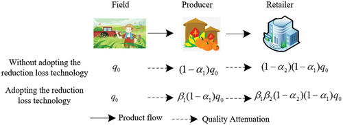
(5) In Figure 1, by the producer’s transportation, air drying and storage, when the food arrives at retailers, we assume that before and after adopting the GPHL reduction technology, the quality of food decay into $(1-{\alpha }_1)q_0$ and ${\beta }_1(1-{\alpha }_1)q_0$, respectively. Here, $1\ge {\beta }_1(1-{\alpha }_1)\ge (1-{\alpha }_1)\ge 0$. Similarly, through the retailer’s transportation and storage, when the food arrives at consumers, we assume that before and after adopting the GPHL reduction technology, the quality of food decay into $(1-{\alpha }_2)(1-{\alpha }_1)q_0$ and ${\beta }_1{\beta }_2(1-{\alpha }_2)(1-{\alpha }_1)q_0$, respectively.Here, $1\ge {\beta }_2{\beta }_1(1-{\alpha }_2)(1-{\alpha }_1)\ge (1-{\alpha }_2)(1-{\alpha }_1)\ge 0$.

Figure 1. Deterioration situation of food quality in the two loss reduction backgrounds.

(6) The reduction of quality loss $\mathrm{\Delta }q$ is $({\beta }_1-1)(1-{\alpha }_1)q_0$, and the reduction level of quality loss is $\mathrm{\Delta }q/(1-{\alpha }_1)q_0=({\beta }_1-1)$. Similar to Chen & Chen (2020), we assume that the loss reduction cost of the producer $c_2={\kappa }_2{({\beta }_1-1)}^2/2$. In the same way, the loss reduction cost of the retailer $c_3={\kappa }_3{({\beta }_2-1)}^2/2$.

(7) Considering the data obtaining convenience about food loss reduction cost, we propose to use the food quality loss reduction cost and quantity loss reduction cost to reflect the inputs of food loss reduction. Namely, the loss reduction cost of the producer equals to $C({\delta }_1,{\beta }_1)=C_1+c_2=$ ${\kappa }_1{(1-{\delta }_1)}^2/2+{\kappa }_2{({\beta }_1-1)}^2/2$, and the loss reduction cost of the retailer equals to $C({\delta }_2,{\beta }_2)=C_2+c_3=$${\kappa }_4{(1-{\delta }_2)}^2/2+{\kappa }_3{({\beta }_2-1)}^2/2$.

(8) Similar to Nie (2012) and Zhang et al. (2020), it is assumed that the demand formula can be as $D^i=\frac{M}{{(1-\gamma )}^y{e}_0}-p_i-({\beta }_1{)}^{z_1}({\beta }_2{)}^{z_2}(1-{\alpha }_1{)}^{z_3}(1-{\alpha }_2{)}^{z_4}{q}_0$. $y=\{0,1\}$, and when $i=\{NEL\}$, $\mathrm{y}=0$. When $i=\{ENL,EL,ELB\}$, $y=1$. When $i=\{NEL,ENL\}$, ${\mathrm{z}}_4=1$, ${\mathrm{z}}_3=1$, ${\mathrm{z}}_2=0$ and ${\mathrm{z}}_1=0$. When $i=\{EL\}$, ${\mathrm{z}}_4=1$, ${\mathrm{z}}_3=1$, ${\mathrm{z}}_2=0$ and ${\mathrm{z}}_1=1$. When $i=\{ELB\}$, ${\mathrm{z}}_4=1$, ${\mathrm{z}}_3=1$, ${\mathrm{z}}_2=1$ and ${\mathrm{z}}_1=1$.

(9) Consumer surplus is an important indicator of consumer welfare. Consumer surplus is the difference between the maximum price that consumers are willing to pay for a given quantity of goods and the actual market price of the goods. Consumer surplus is as follows:

$CS=\underset{p_i}{\overset{p_{mas}}{\int }}{D}_{i}dp=\frac{D_i^2}{2}$

(10) Assume that the food demand is in tight equilibrium, that is, output is saleable.

3.2. Subsidy analysis

3.2.1. NEL model

In the NEL model, the food producer will not implement the environment innovation investment and the GPHL reduction technology. Profits’ functions of the food producer, the retailer and the government are as follows:

(1) ${\pi }_p^{NEL}=(w^{NEL}-c+\beta )D^{NEL}(1-{\lambda }_1)$(1)

(2) ${\pi }_r^{NEL}=(p^{NEL}-w)D^{NEL}(1-{\lambda }_2)(1-{\lambda }_1)$(2)

(3) ${\pi }_g^{NEL}={\pi }_p^{NEL}+{\pi }_r^{NEL}+C{S}^{NEL}-\beta D^{NEL}$(3)

From equations (1)(1) ${\pi }_p^{NEL}=(w^{NEL}-c+\beta )D^{NEL}(1-{\lambda }_1)$(1) , (2(2) ${\pi }_r^{NEL}=(p^{NEL}-w)D^{NEL}(1-{\lambda }_2)(1-{\lambda }_1)$(2) ) and (3(3) ${\pi }_g^{NEL}={\pi }_p^{NEL}+{\pi }_r^{NEL}+C{S}^{NEL}-\beta D^{NEL}$(3) ), we can get proposition 1 (The analysis process sees Appendix A-1).

Proposition 1.

In the NEL model, the optimal decision about equilibrium prices, benefits of the food producer, the retailer and the government are as follows.

(4) $\left\{\begin{array}{c}{p}^{NEL\ast }=\frac{3M-e_0(\beta -c)+3e_0{q}_0(1-{\alpha }_1-{\alpha }_2+{\alpha }_1{\alpha }_2)}{4e_0}\\ w^{NEL\ast }=\frac{M-e_0(\beta -c)+e_0{q}_0(1-{\alpha }_1-{\alpha }_2+{\alpha }_1{\alpha }_2)}{2e_0}\\ D_{\hspace{0.17em}}^{NEL\ast }=\frac{A}{4e_0}\end{array}\right.$(4)

(5) $\left\{\begin{array}{c}{\pi }_r^{NEL\ast }=\frac{(1-{\lambda }_1)(1-{\lambda }_2)A^2}{16{(e_0)}^2}\\ {\pi }_p^{NEL\ast }=\frac{(1-{\lambda }_1)A^2}{8{(e_0)}^2}\\ {\pi }_g^{NEL\ast }=\frac{A^2[2(1-{\lambda }_1)(1-{\lambda }_2)+4(1-{\lambda }_1)+1]}{32{(e_0)}^2}-\frac{\beta A}{4e_0}\end{array}\right.$(5)

Here, $A=M+e_0(\beta -c)+e_0{q}_0(1-{\alpha }_1-{\alpha }_2+{\alpha }_1{\alpha }_2)$.

3.2.2. ENL model

In the ENL model, the food producer will implement the environment innovation investment, but it will not adopt the GPHL reduction technology. Revenue functions of the food producer, the retailer and the government are as follows:

(6) ${\pi }_p^{ENL}=(w^{ENL}-c+\beta )D^{ENL}(1-{\lambda }_1)-\frac{(1-s)k{\gamma }^2}{2}$(6)

(7) ${\pi }_r^{ENL}=(p^{ENL}-w^{ENL})D^{ENL}(1-{\lambda }_1)(1-{\lambda }_2)$(7)

(8) ${\pi }_g^{ENL}={\pi }_p^{ENL}+{\pi }_r^{ENL}+C{S}^{ENL}-\beta D^{ENL}-\frac{sk{\gamma }^2}{2}$(8)

From equations (1)(1) ${\pi }_p^{NEL}=(w^{NEL}-c+\beta )D^{NEL}(1-{\lambda }_1)$(1) , (6(6) ${\pi }_p^{ENL}=(w^{ENL}-c+\beta )D^{ENL}(1-{\lambda }_1)-\frac{(1-s)k{\gamma }^2}{2}$(6) ), (7(7) ${\pi }_r^{ENL}=(p^{ENL}-w^{ENL})D^{ENL}(1-{\lambda }_1)(1-{\lambda }_2)$(7) ) and (8(8) ${\pi }_g^{ENL}={\pi }_p^{ENL}+{\pi }_r^{ENL}+C{S}^{ENL}-\beta D^{ENL}-\frac{sk{\gamma }^2}{2}$(8) ), we can get proposition 2 (The analysis process is similar to it in Proposition 1).

Proposition 2.

In the ENL model, the optimal decision about equilibrium prices, benefits of the food producer, the retailer and the government are as follows.

(9) $\left\{\begin{array}{c}{w}^{ENL\ast }=-\frac{(\beta -c)}{2}-B\\ p^{ENL\ast }=\frac{\beta -c}{4}-\frac{3B}{2}\\ D_{\hspace{0.17em}}^{NEL\ast }=\frac{E}{4{\mathrm{e}}_0(1-\gamma )}\end{array}\right.$(9)

(10) $\left\{\begin{array}{c}{\pi }_p^{ENL\ast }=\frac{(1-{\lambda }_1)E^2}{8{(e_0)}^2{(1-\gamma )}^2}-\frac{(1-s)k{\gamma }^2}{2}\\ {\pi }_r^{ENL\ast }=\frac{(1-{\lambda }_1)(1-{\lambda }_2)E^2}{16{(e_0)}^2{(1-\gamma )}^2}\\ {\pi }_g^{ENL\ast }=\frac{E^2[(1-{\lambda }_1)(1-{\lambda }_2)+2(1-{\lambda }_1)+2]}{32{(e_0)}^2{(1-\gamma )}^2}-\frac{k{\gamma }^2}{2}-\frac{\beta E}{4e_0(1-\gamma )}\end{array}\right.$(10)

Here, $B=-\frac{q_0(1-{\alpha }_1)(1-{\alpha }_2)}{2}-\frac{M}{2e_0(1-\gamma )}<0$ and $E=M+e_0{q}_0(1-\gamma )(1-{\alpha }_1-{\alpha }_2+{\alpha }_1{\alpha }_2)+e_0({\beta }_1-c)(1-\gamma )$.

According to proposition 2, we can get inference 1 (The analysis process sees Appendix B-1).

Inference 1. ① $\frac{\mathrm{\partial }{p}^{ENL\ast }}{\mathrm{\partial }s}=0,\frac{\mathrm{\partial }{w}^{ENL\ast }}{\mathrm{\partial }s}=0,\frac{\mathrm{\partial }{\pi }_r^{ENL\ast }}{\mathrm{\partial }s}=0,\frac{\mathrm{\partial }{\pi }_p^{ENL\ast }}{\mathrm{\partial }s}>0,\frac{\mathrm{\partial }{\pi }_g^{ENL\ast }}{\mathrm{\partial }s}=0;$②$\frac{\mathrm{\partial }{p}^{ENL\ast }}{\mathrm{\partial }\gamma }>0,\frac{\mathrm{\partial }{w}^{ENL\ast }}{\mathrm{\partial }\gamma }>0,\frac{\mathrm{\partial }{\pi }_r^{ENL\ast }}{\mathrm{\partial }\gamma }>0,\frac{\mathrm{\partial }{\pi }_p^{ENL\ast }}{\mathrm{\partial }\gamma }>0,\frac{\mathrm{\partial }{\pi }_g^{ENL\ast }}{\mathrm{\partial }\gamma }>0.$

From ① in the inference 1, we can understand that the environmental innovation subsidy coefficient will not influence the change trends of the equilibrium prices and the benefits of the retailer and the government, however, it will affect the producer incomes. At the same time, with the growth of the environmental innovation subsidy coefficient, benefits of the producer will add. It is possible because the environmental innovation subsidy is to subsidize the inputs of the environmental innovation of the producer; thus, benefits of the retailer have no relationship with it, and the producer’s benefits will add. The government’s incomes are composed of chain members’ incomes, consumer surplus and the related subsidy expenditure. The mixture of these incomes and expenditure will eliminate the influences of the environmental innovation subsidy coefficient on the government’s incomes.

From ② in the inference 1, with the increase of the effort level of PE reduction, the prices about food will grow. Meanwhile, from the appendix B-1, it can be known that with the change of the effort level of PE reduction, the change region of the wholesale price is bigger than the retail prices. It may be because the increase of the effort level of PE reduction needs the producer to invest in more environmental innovation costs; therefore, the producer must set a high wholesale price, and so does the retailer. In addition, with the increase of the effort level of PE reduction, the incomes of the producer, the retailer and the government will increase. It is possible because under a certain limit condition about PE, the rise of the effort level of PE reduction will help the producer gain more production spaces, and they can produce more gains. If the demand is in tight equilibrium, the production growth will help the retailer and the producer gain more revenues. The income rise of the retailer and the producer will make the government gain more social benefits.

3.2.3. EL model

In the EL model, the food producer will implement the environment innovation investment and adopt the GPHL reduction technology. Revenue functions of the food producer, the retailer and government are as follows:

(11) ${\pi }_p^{EL}=(w^{EL}-c+\beta )D^{EL}(1-{\delta }_1{\lambda }_1)-\frac{(1-s)k{\gamma }^2}{2}-\frac{(1-s_1)[k_1{({\delta }_1-1)}^2+k_2{({\beta }_1-1)}^2]}{2}$(11)

(12) ${\pi }_r^{EL}=(p^{EL}-w^{EL})D^{EL}(1-{\delta }_1{\lambda }_1)(1-{\lambda }_2)$(12)

(13) ${\pi }_g^{EL}={\pi }_p^{EL}+{\pi }_r^{EL}+C{S}^{EL}-\beta D^{EL}-\frac{sk{\gamma }^2}{2}-\frac{s_1[k_1{({\delta }_1-1)}^2+k_2{({\beta }_1-1)}^2]}{2}$(13)

From equations (1)(1) ${\pi }_p^{NEL}=(w^{NEL}-c+\beta )D^{NEL}(1-{\lambda }_1)$(1) , (11(11) ${\pi }_p^{EL}=(w^{EL}-c+\beta )D^{EL}(1-{\delta }_1{\lambda }_1)-\frac{(1-s)k{\gamma }^2}{2}-\frac{(1-s_1)[k_1{({\delta }_1-1)}^2+k_2{({\beta }_1-1)}^2]}{2}$(11) ), (12(12) ${\pi }_r^{EL}=(p^{EL}-w^{EL})D^{EL}(1-{\delta }_1{\lambda }_1)(1-{\lambda }_2)$(12) ) and (13(13) ${\pi }_g^{EL}={\pi }_p^{EL}+{\pi }_r^{EL}+C{S}^{EL}-\beta D^{EL}-\frac{sk{\gamma }^2}{2}-\frac{s_1[k_1{({\delta }_1-1)}^2+k_2{({\beta }_1-1)}^2]}{2}$(13) ), we can get proposition 3 (The analysis process is similar to it in Proposition 1).

Proposition 3.

In the EL model, the optimal decision about equilibrium prices, benefits of the food producer, the retailer and the government are as follows.

(14) $\left\{\begin{array}{c}{w}^{EL\ast }=-\frac{(\beta -c)}{2}-B_1\\ p^{EL\ast }=\frac{\beta -c}{4}-\frac{B_1}{4}\\ D_{\hspace{0.17em}}^{NL\ast }=\frac{E_1}{4{\mathrm{e}}_0(1-\gamma )}\end{array}\right.$(14)

(15) $\left\{\begin{array}{c}{\pi }_p^{EL\ast }=\frac{(1-{\delta }_1{\lambda }_1){(E_1)}^2}{8{(e_0)}^2{(1-\gamma )}^2}-\frac{(1-s)k{\gamma }^2}{2}-\frac{(1-s_1)[k_1{({\delta }_1-1)}^2+k_2{({\beta }_1-1)}^2]}{2}\\ {\pi }_r^{EL\ast }=\frac{(1-{\delta }_1{\lambda }_1)(1-{\lambda }_2){(E_1)}^2}{16{(e_0)}^2{(1-\gamma )}^2}\\ {\pi }_g^{EL\ast }=\frac{{(E_1)}^2[2(1-{\delta }_1{\lambda }_1)(1-{\lambda }_2)+4(1-{\delta }_1{\lambda }_1)+1]}{32{(e_0)}^2{(1-\gamma )}^2}-\frac{k{\gamma }^2+k_1{({\delta }_1-1)}^2+k_2{({\beta }_1-1)}^2}{2}-\frac{\beta E_1}{4e_0(1-\gamma )}\end{array}\right.$(15)

Here, $B_1=\frac{{\beta }_1{q}_0(1-{\alpha }_1)(1-{\alpha }_2)}{2}-\frac{M}{2e_0(1-\gamma )}<0\mathrm{a}\mathrm{n}\mathrm{d}$$E_1=M+e_0(\beta -c)(1-\gamma )-e_0{q}_0{\beta }_1(1-\gamma )(1-{\alpha }_1-{\alpha }_2+{\alpha }_1{\alpha }_2)$.

According to proposition 3, we can get inference 2 (The analysis process is similar to it in Inference 1).

Inference 2. ① $\frac{\mathrm{\partial }{p}^{EL\ast }}{\mathrm{\partial }s}=0,\frac{\mathrm{\partial }{w}^{EL\ast }}{\mathrm{\partial }s}=0,\frac{\mathrm{\partial }{\pi }_r^{EL\ast }}{\mathrm{\partial }s}=0,\frac{\mathrm{\partial }{\pi }_p^{EL\ast }}{\mathrm{\partial }s}>0,\frac{\mathrm{\partial }{\pi }_g^{EL\ast }}{\mathrm{\partial }s}=0;$

② $\frac{\mathrm{\partial }{p}^{EL\ast }}{\mathrm{\partial }\gamma }>0,\frac{\mathrm{\partial }{w}^{EL\ast }}{\mathrm{\partial }\gamma }>0,\frac{\mathrm{\partial }{\pi }_r^{EL\ast }}{\mathrm{\partial }\gamma }>0,\frac{\mathrm{\partial }{\pi }_p^{EL\ast }}{\mathrm{\partial }\gamma }>0,\frac{\mathrm{\partial }{\pi }_g^{EL\ast }}{\mathrm{\partial }\gamma }>0.$

③ $\frac{\mathrm{\partial }{p}^{EL\ast }}{\mathrm{\partial }{\delta }_1}=0,\frac{\mathrm{\partial }{w}^{EL\ast }}{\mathrm{\partial }{\delta }_1}=0,\frac{\mathrm{\partial }{\pi }_r^{EL\ast }}{\mathrm{\partial }{\delta }_1}<0,\frac{\mathrm{\partial }{\pi }_p^{EL\ast }}{\mathrm{\partial }{\delta }_1}<0,\frac{\mathrm{\partial }{\pi }_g^{EL\ast }}{\mathrm{\partial }{\delta }_1}<0.$

④ $\frac{\mathrm{\partial }{p}^{EL\ast }}{\mathrm{\partial }{\beta }_1}>0,\frac{\mathrm{\partial }{w}^{EL\ast }}{\mathrm{\partial }{\beta }_1}>0,\frac{\mathrm{\partial }{\pi }_r^{EL\ast }}{\mathrm{\partial }{\beta }_1}>0,\frac{\mathrm{\partial }{\pi }_p^{EL\ast }}{\mathrm{\partial }{\beta }_1}>0,\frac{\mathrm{\partial }{\pi }_g^{EL\ast }}{\mathrm{\partial }{\beta }_1}>0.$

⑤ $\frac{\mathrm{\partial }{p}^{EL\ast }}{\mathrm{\partial }{s}_1}=0,\frac{\mathrm{\partial }{w}^{EL\ast }}{\mathrm{\partial }{s}_1}=0,\frac{\mathrm{\partial }{\pi }_r^{EL\ast }}{\mathrm{\partial }{s}_1}=0,\frac{\mathrm{\partial }{\pi }_p^{EL\ast }}{\mathrm{\partial }{s}_1}>0,\frac{\mathrm{\partial }{\pi }_g^{EL\ast }}{\mathrm{\partial }{s}_1}=0.$

From ① in the inferences 1 and 2, we can know that in the models of EL and ENL, with growth of the environmental innovation subsidy coefficient, decision variables (prices) and dependent variables (benefits) have the same change tendency. Namely, in the two models, the environmental innovation subsidy coefficient will not influence the change trends of the equilibrium prices and the benefits of the retailer and the government. At the same time, with the growth of the environmental innovation subsidy coefficient, benefits of the producer will add; moreover, the change spaces are same under the two models.

From ② in the inferences 1 and 2, in the models of EL and ENL, with the growth of the effort level of PE reduction, decision variables (prices) and dependent variables (benefits) have the same change tendency. In addition, with the change of the effort level of PE reduction, in the two models, the change regions about the wholesale price and the retail price are same. This tells us that with the increase of the effort level of PE reduction, the change magnitudes about the equilibrium prices will not be affected by investing in the GPHL reduction technology. However, in the two models, with the increase of the effort level of PE reduction, the change magnitudes about the chain members’ incomes are different.

From ③ in the inferences 2, the discount rate of the unit quantity loss of the producer ${\delta }_1$ has no relationship with the decision variables (prices $p^{EL\ast }$ and $w^{EL\ast }$) and has a negative correlation with the dependent variables (benefits ${\pi }_r^{EL\ast }$, ${\pi }_p^{EL\ast }$ and ${\pi }_g^{EL\ast }$). It may be because the bigger the discount rate of the unit quantity loss of the producer${\delta }_1$, the more the unit quantity loss. Thus, the dependent variables (benefits ${\pi }_r^{EL\ast }$, ${\pi }_p^{EL\ast }$ and${\pi }_g^{EL\ast }$) will be lower. The smaller the discount rate of the unit quantity loss of the producer ${\delta }_1$, the bigger the improvement rate of the unit quantity loss of the producer, and the little the unit quantity loss.

From ④ in the inferences 2, the quality loss reduction coefficient of the producer ${\beta }_1$ has positive relationships with the decision variables (prices $p^{EL\ast }$ and $w^{EL\ast }$) and the dependent variables (benefits ${\pi }_r^{EL\ast }$, ${\pi }_p^{EL\ast }$ and ${\pi }_g^{EL\ast }$). It may be because the bigger the quality loss reduction coefficient of the producer${\beta }_1$, the slower the food quality decreases, and the bigger the product is accepted by consumers. Thus, to make up for the inputs because of using the GPHL reduction technology, the producer can set a higher wholesale price, and the retailer also needs to set a high retailer price. Then, with the increase of the retail price and the wholesale price, the dependent variables (benefits${\pi }_r^{EL\ast }$, ${\pi }_p^{EL\ast }$ and${\pi }_g^{EL\ast }$) will be added.

From ⑤ in the inference 2, we can understand that the GPHL reduction subsidy coefficient for the producer $s_1$ will not influence the change trends of the equilibrium prices and the benefits of the retailer and the government, however, it will affect the producer incomes. At the same time, with the growth of the GPHL reduction subsidy coefficient for the producer$s_1$, benefits of the producer will add. It is possible because the GPHL reduction subsidy is to subsidize the inputs of the GPHL reduction input of the producer, and benefits of the retailer have no relationship with it, and the producer’s benefits will add. The government’s incomes are composed of supply chain member incomes, consumer surplus and the related subsidy expenditure. The mixture of these incomes and expenditure will eliminate the influences of the GPHL reduction subsidy coefficient on government’s incomes.

3.2.4. ELB model

In the ELB model, the food producer will implement the environment innovation investment and adopt the GPHL reduction technology, and the retailer will also adopt the GPHL reduction technology. Revenue functions of the food producer, the retailer and the government are as follows:

(16) ${\pi }_p^{ELB}=(w^{ELB}-c+\beta )D^{ELB}(1-{\delta }_1{\lambda }_1)-\frac{(1-s)k{\gamma }^2}{2}-\frac{(1-s_1)[k_1{(1-{\delta }_1)}^2+k_2{({\beta }_{`}-1)}^2]}{2}$(16)

(17) ${\pi }_r^{ELB}=(p^{ELB}-w^{ELB})D^{ELB}(1-{\delta }_1{\lambda }_1)(1-{\delta }_2{\lambda }_2)-\frac{(1-s_2)[k_4{(1-{\delta }_2)}^2+k_3{({\beta }_2-1)}^2]}{2}$(17)

(18) ${\pi }_g^{ELB}={\pi }_p^{ELB}+{\pi }_r^{ELB}+C{S}^{ELB}-\beta D^{ELB}-\frac{sk{\gamma }^2}{2}-\frac{s_1[k_1{(1-{\delta }_1)}^2+k_2{({\beta }_{`}-1)}^2]}{2}-\frac{s_2[k_4{(1-{\delta }_2)}^2+k_3{({\beta }_2-1)}^2]}{2}$(18)

From equations (1)(1) ${\pi }_p^{NEL}=(w^{NEL}-c+\beta )D^{NEL}(1-{\lambda }_1)$(1) , (16(16) ${\pi }_p^{ELB}=(w^{ELB}-c+\beta )D^{ELB}(1-{\delta }_1{\lambda }_1)-\frac{(1-s)k{\gamma }^2}{2}-\frac{(1-s_1)[k_1{(1-{\delta }_1)}^2+k_2{({\beta }_{`}-1)}^2]}{2}$(16) ), (17(17) ${\pi }_r^{ELB}=(p^{ELB}-w^{ELB})D^{ELB}(1-{\delta }_1{\lambda }_1)(1-{\delta }_2{\lambda }_2)-\frac{(1-s_2)[k_4{(1-{\delta }_2)}^2+k_3{({\beta }_2-1)}^2]}{2}$(17) ) and (18(18) ${\pi }_g^{ELB}={\pi }_p^{ELB}+{\pi }_r^{ELB}+C{S}^{ELB}-\beta D^{ELB}-\frac{sk{\gamma }^2}{2}-\frac{s_1[k_1{(1-{\delta }_1)}^2+k_2{({\beta }_{`}-1)}^2]}{2}-\frac{s_2[k_4{(1-{\delta }_2)}^2+k_3{({\beta }_2-1)}^2]}{2}$(18) ), we can get proposition 4 (The analysis process is similar to it in Proposition 1).

Proposition 4.

In the ELB model, the optimal decision about equilibrium prices, benefits of the food producer, the retailer and the government are as follows.

(19) $\left\{\begin{array}{c}{w}^{ELB\ast }=\frac{(\beta -c)}{2}+B_2\\ p^{ELB\ast }=\frac{\beta -c}{4}-\frac{3B_2}{4}\\ D_{\hspace{0.17em}}^{NLB\ast }=\frac{E_2}{4{\mathrm{e}}_0(1-\gamma )}\end{array}\right.$(19)

(20) $\left\{\begin{array}{c}{\pi }_p^{ELB\ast }=\frac{(1-{\delta }_1{\lambda }_1)E_2^2}{8{({\mathrm{e}}_0)}^2{(1-\gamma )}^2}-\frac{(1-s)k{\gamma }^2}{2}-\frac{(1-s_1)[k_2{(1-{\beta }_1)}^2+k_1{(1-{\delta }_1)}^2]}{2}\\ {\pi }_r^{ELB\ast }=\frac{(1-{\delta }_1{\lambda }_1)(1-{\delta }_2{\lambda }_2)E_2^2}{16{({\mathrm{e}}_0)}^2{(1-\gamma )}^2}-\frac{(1-s_2)[k_3{(1-{\beta }_2)}^2+k_4{(1-{\delta }_2)}^2]}{2}\\ {\pi }_g^{ELB\ast }=\frac{E_2^2[2(1-{\delta }_1{\lambda }_1)(1-{\delta }_2{\lambda }_2)+4(1-{\delta }_1{\lambda }_1)+1]}{32{({\mathrm{e}}_0)}^2{(1-\gamma )}^2}-\frac{k{\gamma }^2+[k_2{(1-{\beta }_1)}^2+k_1{(1-{\delta }_1)}^2]+[k_3{(1-{\beta }_2)}^2+k_4{(1-{\delta }_2)}^2]}{2}-\frac{\beta E_2}{4e_0(1-\gamma )}\end{array}\right.$(20)

Here, $B_2=\frac{{\beta }_2{\beta }_1{q}_0(1-{\alpha }_1)(1-{\alpha }_2)}{2}-\frac{M}{2e_0(1-\gamma )}<0$, and $E_2=M+e_0(\beta -c)(1-\gamma )-e_0{q}_0{\beta }_1{\beta }_2(1-\gamma )(1-{\alpha }_1-{\alpha }_2+{\alpha }_1{\alpha }_2)$.

According to proposition 4, we can get inference 3 (The analysis process is similar to it in Inference 1).

Inference 3. ① $\frac{\mathrm{\partial }{p}^{ELB\ast }}{\mathrm{\partial }s}=0,\frac{\mathrm{\partial }{w}^{ELB\ast }}{\mathrm{\partial }s}=0,\frac{\mathrm{\partial }{\pi }_r^{ELB\ast }}{\mathrm{\partial }s}=0,\frac{\mathrm{\partial }{\pi }_p^{ELB\ast }}{\mathrm{\partial }s}>0,\frac{\mathrm{\partial }{\pi }_g^{EL\ast }}{\mathrm{\partial }s}=0;$

②$\frac{\mathrm{\partial }{p}^{ELB\ast }}{\mathrm{\partial }\gamma }>0,\frac{\mathrm{\partial }{w}^{EL\ast }}{\mathrm{\partial }\gamma }>0,\frac{\mathrm{\partial }{\pi }_r^{EL\ast }}{\mathrm{\partial }\gamma }>0,\frac{\mathrm{\partial }{\pi }_p^{EL\ast }}{\mathrm{\partial }\gamma }>0,\frac{\mathrm{\partial }{\pi }_g^{EL\ast }}{\mathrm{\partial }\gamma }>0.$

③$\frac{\mathrm{\partial }{p}^{EL\ast }}{\mathrm{\partial }{\delta }_1}=0,\frac{\mathrm{\partial }{w}^{EL\ast }}{\mathrm{\partial }{\delta }_1}=0,\frac{\mathrm{\partial }{\pi }_r^{EL\ast }}{\mathrm{\partial }{\delta }_1}<0,\frac{\mathrm{\partial }{\pi }_p^{EL\ast }}{\mathrm{\partial }{\delta }_1}<0,\frac{\mathrm{\partial }{\pi }_g^{EL\ast }}{\mathrm{\partial }{\delta }_1}<0.$

④$\frac{\mathrm{\partial }{p}^{EL\ast }}{\mathrm{\partial }{\beta }_1}>0,\frac{\mathrm{\partial }{w}^{EL\ast }}{\mathrm{\partial }{\beta }_1}>0,\frac{\mathrm{\partial }{\pi }_r^{EL\ast }}{\mathrm{\partial }{\beta }_1}>0,\frac{\mathrm{\partial }{\pi }_p^{EL\ast }}{\mathrm{\partial }{\beta }_1}>0,\frac{\mathrm{\partial }{\pi }_g^{EL\ast }}{\mathrm{\partial }{\beta }_1}>0.$

⑤$\frac{\mathrm{\partial }{p}^{EL\ast }}{\mathrm{\partial }{s}_1}=0,\frac{\mathrm{\partial }{w}^{EL\ast }}{\mathrm{\partial }{s}_1}=0,\frac{\mathrm{\partial }{\pi }_r^{EL\ast }}{\mathrm{\partial }{s}_1}=0,\frac{\mathrm{\partial }{\pi }_p^{EL\ast }}{\mathrm{\partial }{s}_1}>0,\frac{\mathrm{\partial }{\pi }_g^{EL\ast }}{\mathrm{\partial }{s}_1}=0.$

⑥$\frac{\mathrm{\partial }{p}^{ELB\ast }}{\mathrm{\partial }{\delta }_2}=0,\frac{\mathrm{\partial }{w}^{ELB\ast }}{\mathrm{\partial }{\delta }_2}=0,\frac{\mathrm{\partial }{\pi }_r^{ELB\ast }}{\mathrm{\partial }{\delta }_2}<0,\frac{\mathrm{\partial }{\pi }_p^{ELB\ast }}{\mathrm{\partial }{\delta }_2}<0,\frac{\mathrm{\partial }{\pi }_g^{ELB\ast }}{\mathrm{\partial }{\delta }_2}<0.$

⑦$\frac{\mathrm{\partial }{p}^{ELB\ast }}{\mathrm{\partial }{\beta }_2}>0,\frac{\mathrm{\partial }{w}^{ELB\ast }}{\mathrm{\partial }{\beta }_2}>0,\frac{\mathrm{\partial }{\pi }_r^{ELB\ast }}{\mathrm{\partial }{\beta }_2}>0,\frac{\mathrm{\partial }{\pi }_p^{ELB\ast }}{\mathrm{\partial }{\beta }_2}>0,\frac{\mathrm{\partial }{\pi }_g^{ELB\ast }}{\mathrm{\partial }{\beta }_2}>0.$

⑧$\frac{\mathrm{\partial }{p}^{ELB\ast }}{\mathrm{\partial }{s}_2}=0,\frac{\mathrm{\partial }{w}^{ELB\ast }}{\mathrm{\partial }{s}_2}=0,\frac{\mathrm{\partial }{\pi }_r^{ELB\ast }}{\mathrm{\partial }{s}_2}>0,\frac{\mathrm{\partial }{\pi }_p^{ELB\ast }}{\mathrm{\partial }{s}_2}=0,\frac{\mathrm{\partial }{\pi }_g^{ELB\ast }}{\mathrm{\partial }{s}_2}=0.$

From ① in the inferences 1, 2 and 3, we can get that in the models of EL, ELB and ENL, the environmental innovation subsidy coefficient will not influence the change trends of equilibrium prices and the benefits of the retailer and the government. At the same time, with the growth of the environmental innovation subsidy coefficient, the producer benefits will add; moreover, the change spaces are same under the three models. These demonstrate that for the producer, the change trends of decision variables (prices) and dependent variables (benefits) with the growth of the environmental innovation subsidy coefficient will not be affected by chain members’ investment behavior about the GPHL reduction technology.

From ② in the inferences 1, 2 and 3, in the models of EL, ELB and ENL, with the increase of the effort level of PE reduction, the retail price and the wholesale price about food will grow. Meanwhile, with the change of the effort level of PE reduction, in the three models, the change regions about the wholesale price and the retail price are same. However, in the three models, with the increase of the effort level of PE reduction, the change magnitudes about the chain members’ incomes are different. This tells us that with the increase of the effort level of PE reduction, the change magnitudes about the chain members’ incomes will be affected by the retailer investment behavior.

From ③ in the inferences 2 and 3, in the models of EL and ELB, the discount rate of the unit quantity loss of the producer ${\delta }_1$ has no relationship with the decision variables (prices $p^{EL\ast }$ and $w^{EL\ast }$) and has a negative correlation with the dependent variables (benefits ${\pi }_r^{EL\ast }$, ${\pi }_p^{EL\ast }$ and ${\pi }_g^{EL\ast }$). This tells us that with the rise of the unit quantity loss discount rate of the producer, the change tendency and magnitudes about the equilibrium prices will not be affected by the retailer’s investment behavior about the GPHL reduction technology, but the change magnitudes about the chain members’ incomes will be affected by the retailer’s investment behavior.

From ④ in the inferences 2 and 3, in the models of EL and ELB, the quality loss reduction coefficient of the producer ${\beta }_1$ has positive relationships with the decision variables (prices $p^{EL\ast }$ and $w^{EL\ast }$) and the dependent variables (benefits ${\pi }_r^{EL\ast }$, ${\pi }_p^{EL\ast }$ and ${\pi }_g^{EL\ast }$). This indicates that with the rise of the quality loss reduction coefficient in the producer, the change tendency about the equilibrium prices and the chain members’ incomes will not be affected by the retailer’s investment behavior on the GPHL reduction technology, but the change magnitudes about the equilibrium prices and the chain members’ incomes will be affected by the retailer’s investment behavior.

From ⑤ in the inference 2 and 3, in the models of EL and ELB, we can understand that the GPHL reduction subsidy coefficient for the producer $s_1$ will not influence the change trends of the equilibrium prices and benefits of the retailer and the government, however, it will affect the producer incomes. With the growth of the GPHL reduction subsidy coefficient for the producer$s_1$, the producer benefits will add. This indicates that with the rise of the GPHL reduction subsidy coefficient for the producer, the change tendency and magnitudes about the equilibrium prices and the incomes of the retailer and the government will not be affected by the retailer’s investment behavior on the GPHL reduction technology, but the change magnitudes about the producer’s incomes will be affected by the retailer’s investment behavior.

From ⑥ in the inferences 3, the quantity loss discount rate of the retailer ${\delta }_2$ has no relationship with the decision variables (prices $p^{ELB\ast }$ and $w^{ELB\ast }$) and has a negative correlation with the dependent variables (benefits ${\pi }_r^{ELB\ast }$, ${\pi }_p^{ELB\ast }$ and ${\pi }_g^{ELB\ast }$). It may be because the bigger the quantity loss discount rate of the retailer${\delta }_2$, the more the unit quantity loss. Thus, the dependent variables (benefits${\pi }_r^{ELB\ast }$, ${\pi }_p^{ELB\ast }$ and${\pi }_g^{ELB\ast }$) will be lower. The smaller the quantity loss discount rate of the retailer${\delta }_2$, the bigger the improvement rate of the unit quantity loss of the retailer, and the smaller the unit quantity loss. Thus, if stakeholders want to obtain more incomes, the retailer should make full use of the GPHL reduction technology to reduce the discount rate as much as possible.

From ⑦ in the inferences 3, the quality loss reduction coefficient of the retailer ${\beta }_2$ has positive relationships with the decision variables (prices $p^{ELB\ast }$ and $w^{ELB\ast }$) and the dependent variables (benefits ${\pi }_r^{ELB\ast }$, ${\pi }_p^{ELB\ast }$ and ${\pi }_g^{ELB\ast }$). It may be because the bigger the quality loss reduction coefficient of the retailer${\beta }_2$, the slower the food quality decreases, and the bigger the product is accepted by consumers. Hence, to make up for the inputs because of using the GPHL reduction technology, the retailer must set a high retail price to gain more orders, and the producer may also reduce its wholesale price. And then, with the increase of the retail price and the wholesale price, the dependent variables (benefits${\pi }_r^{ELB\ast }$, ${\pi }_p^{ELB\ast }$ and${\pi }_g^{ELB\ast }$) will be higher. Thus, if stakeholders want to obtain more incomes, the retailer should make full use of the GPHL reduction technology to add the quality loss reduction coefficient as much as possible.

From ⑧ in the inference 3, we can understand that the GPHL reduction subsidy coefficient for the retailer $s_2$ will not influence the change trends of the equilibrium prices and the benefits of the retailer and the government, however, it will affect the retailer incomes. At the same time, with the growth of the GPHL reduction subsidy coefficient for the retailer$s_2$, benefits of the retailer will add. It is possible because the loss reduction subsidy is to subsidy the retailer inputs on his/her loss reduction; thus, benefits of the producer have no relationship with it, and the retailers will add. The government’s incomes are composed of supply chain members’ incomes, consumer surplus and the related subsidy expenditure. The mixture of these incomes and expenditure will eliminate the influences of the GPHL reduction subsidy coefficient on government’s incomes.

3.2.5. Analysis of subsidy strategy

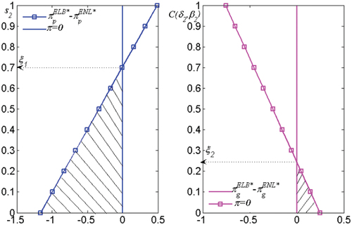
Inference 4. When $1\ge s>{\psi }_1$ and $C(\gamma )<{\psi }_2$ can be met, investing in the PE reduction technology and subsidizing this investment is feasible. (The analysis process sees Appendix C-1).

According to Appendix C-1, we know $s>{\psi }_1$. Based on this, we can get when $\gamma >0.38$, government should offer a high environmental innovation subsidy coefficient $s$ to the producer; otherwise, the producer will refuse to use the PE reduction technology because of the input-output imbalance. When $\gamma <0.38$, government can offer a low environmental innovation subsidy coefficient $s$ to the producer. However, if the cost of the PE reduction technology is higher (e.g., $C(\gamma )>{\psi }_2$), it is not suitable for the government to offer a varying subsidy to the producer. In this condition, government can offer a fixed cost subsidy to the producer or set an upper limit of subsidy.

Inference 5. When $s_1>{\omega }_1$ and $C({\delta }_1,{\beta }_1)<{\omega }_2$, investing in the PE reduction technology and subsidizing this investment is feasible. (The analysis process is similar to it in Inference 4).

According to Appendix C-2, we know $s_1>{\omega }_1$. Based on this, we can get when $q_0(1-{\delta }_1{\lambda }_1)(1-{\alpha }_1)(1-{\alpha }_2)E_1-\frac{2k_2(1-{\beta }_1)[(1-{\delta }_1{\lambda }_1)E_1^2-(1-{\lambda }_1)E^2]}{B{e}_0(1-\gamma )}>0$, with the growth of the loss reduction effort level of the producer ${\beta }_1$, the GPHL reduction subsidy coefficient for the producer $s_1$ will increase. When $B{\lambda }_1{E}_1^2>2k_1(1-{\delta }_1)[(1-{\delta }_1{\lambda }_1)E_1^2-(1-{\lambda }_1)E^2]$, with the rise of the quantity loss discount rate of the producer ${\delta }_1$, the GPHL reduction subsidy coefficient for the producer $s_1$ will increase. Here, $B=2k_1(1-{\delta }_1{)}^2+k_2({\beta }_1-1{)}^2$. These indicate that with the growth of the loss reduction effort level of the producer and the quantity loss discount rate of the producer, it is not always possible to make the government offer a higher loss reduction subsidy coefficient, and only some conditions can be met, the government offer a higher loss reduction subsidy coefficient. In addition, if the cost of the GPHL reduction technology is higher (e.g., $C({\delta }_1,{\beta }_1)>{\omega }_2$), it is not suitable for the government to offer a varying subsidy to the producer. In this condition, government can offer a fixed cost subsidy to the producer or set an upper limit of subsidy.

Inference 6. When $s_2>{\xi }_1$ and $C({\delta }_2,{\beta }_2)<{\xi }_2$, investing in the PE reduction technology and subsidizing this investment is feasible. (The analysis process is similar to it in Inference 4).

According to Appendix C-3, we know $s_2>{\xi }_1$. Based on this, we can get when $q_0(1-{\delta }_1{\lambda }_1)(1-{\alpha }_1)(1-{\alpha }_2)E_1-\frac{2k_3(1-{\beta }_2)[(1-{\delta }_1{\lambda }_1)(1-{\delta }_2{\lambda }_2)E_2^2-(1-{\delta }_1{\lambda }_1)(1-{\lambda }_1)E_1^2]}{B_1{e}_0(1-\gamma )}>0$, with the growth of the loss reduction effort level of the retailer ${\beta }_2$, the GPHL reduction subsidy coefficient for the retailer $s_2$ will increase. When $B_1{\lambda }_2{E}_1^2>2k_4(1-{\delta }_2)[(1-{\delta }_2{\lambda }_2)E_2^2-(1-{\lambda }_2)E_1^2]$, with the rise of the quantity loss discount rate of the retailer ${\delta }_1$, the GPHL reduction subsidy coefficient for the retailer $s_2$ will increase. Here $B_1=2k_3(1-{\delta }_2{)}^2+k_4({\beta }_2-1{)}^2$. In addition, if the cost of the GPHL reduction technology is higher (e.g., $\mathrm{C}({\delta }_2,{\beta }_2)>{\xi }_2$), it is not suitable for the government to offer a varying subsidy to the producer. In this condition, government can offer a fixed cost subsidy to the producer or set an upper limit of subsidy.

4. Case study

4.1. Numerical simulation

Based on the research of Zhang et al. (2020) from China, we set $M=10$, $e_0=0.1$, $\gamma =0.1$ and $\beta =0.02$. According to our survey study about food loss in Shangqiu city of Henan, China, the food quantity loss of Shangqiu city is different for different farmers or producers. For producers who adopt the backward equipment of harvesting and storage, the average rates of the food quantity loss and the food quality loss are about 8% ~18% and 6%~20%, respectively. For producers who adopt the advanced equipment of harvesting and storage, the average rates of the food quantity loss and the food quality loss are less than 3% and 2%, respectively. For the retailer, who adopt the backward storage equipment, the average rates of the food quantity loss and the food quality loss are about 3%~8% and 5%~15%, respectively. For retailers who adopt the advanced storage equipment, the average rates of the food quantity loss and the food quality loss are less than 1% and 1%, respectively. Thus, we set ${\alpha }_1=0.1$, ${\alpha }_2=0.05$, ${\beta }_2=0.2$, ${\beta }_1=0.6$, ${\lambda }_1=0.1$, ${\lambda }_2=0.04$, ${\delta }_1=0.6$ and ${\delta }_2=0.7$. In addition, we assume that $q_0=2$, $c=0.02$, $\mathrm{k}=500$, ${\mathrm{k}}_1=1000$, ${\mathrm{k}}_2=1000$, ${\mathrm{k}}_3=50$, ${\mathrm{k}}_4=50$. Based on the above values and the proposed propositions and inferences, we get the following figures.

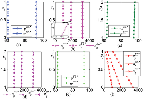
From Figure 2, the changes of the environmental innovation subsidy coefficient will not influence the change trends of equilibrium prices and the benefits of the retailer and the government, however, it will affect the producer incomes. At the same time, with the growth of the environmental innovation subsidy coefficient, the producer benefits will add. Based on these, the environmental innovation subsidy can stimulate the producer to adopt the environmental technology.

Figure 2. Variation trends of equilibrium prices and benefits with $s$ in the NEL model.

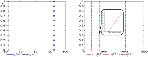
From Figure 3, with the increase of the PE reduction effort level, the retail price and the wholesale price about food will grow. Meanwhile, with the change of the effort level of PE reduction, the change region of the wholesale price about food is bigger than the retail price. In addition, with the increase of the effort level of PE reduction, the incomes of the producer, the retailer and the government will increase. If the demand is in tight equilibrium, the production growth will help the retailer and the producer gain more revenues. The above analyses proved the inference 1.

Figure 3. Variation trends of equilibrium prices and benefits with $\gamma$ in the NEL model.

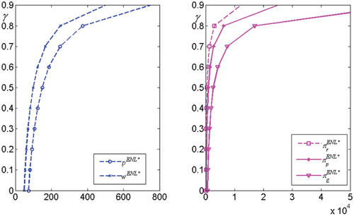
Through comparing Figures 4, 3 and 2, it is understood that under the models of ENL and EL, the environmental innovation subsidy coefficient will not influence the change trends of the equilibrium prices and the benefits of the retailer and the government. This demonstrates that for the producer, the change trends of decision variables (prices) and dependent variables (benefits) with the growth of the environmental innovation subsidy coefficient will not be affected by investing in the GPHL reduction technology.

Figure 4. Variation trends of equilibrium prices and benefits with $\gamma$ and $s$ in the EL model.

In addition, in the models of EL and ENL, with the increase of the effort level of PE reduction, the change trends about the equilibrium prices will not be affected by investing in the GPHL reduction technology. In the two models, with the increase of the effort level of PE reduction, the change magnitudes about the chain members’ incomes will be affected by investing in the GPHL reduction technology.

According to Figure 5, the quantity loss discount rate of the producer ${\delta }_1$ has no relationship with the decision variables (prices) and has a negative correlation with the dependent variables (benefits). Thus, if stakeholders want to obtain more incomes, the producer should make full use of the GPHL reduction technology to reduce the discount rate as much as possible. In addition, the quality loss reduction coefficient of the producer ${\beta }_1$ has positive relationships with the decision variables (prices) and the dependent variables (benefits). Therefore, if stakeholders want to obtain more incomes, the producer should make full use of the GPHL reduction technology to add the quality loss reduction coefficient as much as possible. Meanwhile, we can understand that the GPHL reduction subsidy coefficient for the producer $s_1$ will not influence the change trends of the equilibrium prices and benefits of the retailer and the government, and it will affect the incomes of the producer. With the growth of the GPHL reduction subsidy coefficient for the producer$s_1$, the producer benefits will add. The loss reduction subsidy for the producer can stimulate the producer to adopt the GPHL reduction technology.

Figure 5. Variation trends of equilibrium prices and benefits with ${\beta }_1$, ${\delta }_1$ and $s$ in the EL model.

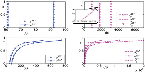
Through comparing Figures 4, 5 and 6, in the models of EL, ELB and ENL, the environmental innovation subsidy coefficient and the effort level of PE reduction will not influence the change trends of the equilibrium prices and the benefits of the retailer and government, but the producer benefits will add; moreover, the change spaces are same under the three models. In addition, in the models of EL and ELB, with the rise of the quality loss reduction coefficient and the unit quantity loss discount rate of the producer, the change tendencies about the equilibrium prices and the chain members’ incomes will not be affect by the retailer’s investment behavior on the GPHL reduction technology, but the change magnitudes about the equilibrium prices and the chain members’ incomes will be affected by the retailer’s investment behavior.

Figure 6. AVariation trends of equilibrium prices and benefits with ${\beta }_1$, ${\delta }_1$, $\gamma$ and $s$ in the ELB model.

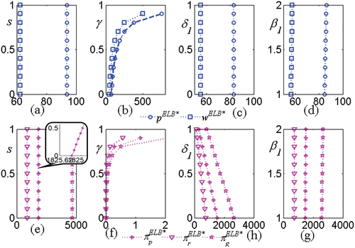
Through comparing Figures 4, 5 and 7, with the rise of the GPHL reduction subsidy coefficient for the producer, the change tendencies and magnitudes about the equilibrium prices and the incomes of the retailer and the government will not be affected by the retailer’s investment behavior on the GPHL reduction technology, but the change magnitudes about the producer’s incomes will be affected by the retailer’s investment behavior. In addition, if stakeholders want to obtain more incomes, the retailer should make full use of the GPHL reduction technology to reduce the discount rate as much as possible. Moreover, the quality loss reduction coefficient of the retailer ${\beta }_2$ has positive relationships with the decision variables (prices) and the dependent variables (benefits). Thus, if stakeholders want to obtain more incomes, the retailer should make full use of the GPHL reduction technology to add the quality loss reduction coefficient as much as possible. Meanwhile, the GPHL reduction subsidy coefficient for the retailer $s_2$ will not influence the change trends of the equilibrium prices and the benefits of the retailer and government, however, it will affect the incomes of the retailer.

Figure 7. Variation trends of equilibrium prices and benefits with ${\beta }_2$, ${\delta }_2$, $s_1$ and $s_2$ in the ELB model.

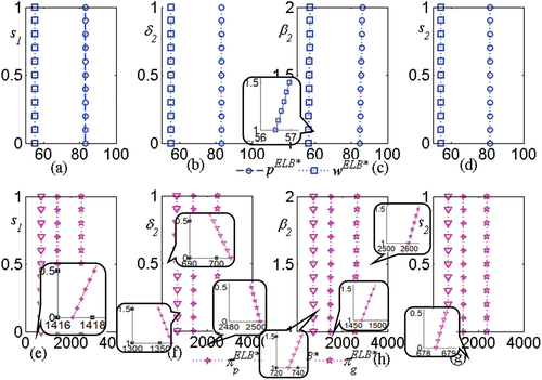
According to Figure 8, when the cost of the PE reduction technology and the environmental innovation subsidy coefficient are in a certain range, the producer will invest in the PE reduction technology and the government will subsidize this investment. If the cost of the PE reduction technology exceeds a certain range (e.g., $C(\gamma )>{\psi }_2$), the varying subsidy is not suitable for the government, and it can offer a fixed subsidy to the producer. Government subsidy for the producer PE reduction investment can increase the profit margin of the producer. Meanwhile, the producer should also try to reduce its PE reduction cost, only in this way, that government offers this varying subsidy model is feasible.

Figure 8. Investment and subsidy conditions of PE technology for the producer.

According to Figure 9, when the cost of the GPHL reduction technology and the GPHL reduction subsidy coefficient for the producer are in a certain range, the producer will invest in the GPHL reduction technology and the government will subsidize this investment. If the cost of the GPHL reduction technology exceeds a certain range (e.g., $C({\delta }_1,{\beta }_1)>{\omega }_2$), the variable subsidy is not suitable for the government, and it can offer a fixed subsidy to the producer. Government subsidy for the producer loss reduction investment can increase the profit margin of the producer.

Figure 9. Investment and subsidy conditions of the GPHL reduction technology for the producer.

According to Figure 10, when the costs of the GPHL reduction technology and the GPHL reduction subsidy coefficient for the retailer are in a certain range, the retailer will invest in the GPHL reduction technology and the government will subsidize this investment. If the GPHL reduction cost exceeds a certain range (e.g., $\mathrm{C}({\delta }_2,{\beta }_2)>{\xi }_2$), the variable subsidy is not suitable for the government, and it can offer a fixed subsidy to the producer. Government subsidy for the retailer’s loss reduction investment can increase the profit margin of the retailer.

Figure 10. Investment and subsidy conditions of the GPHL reduction technology for the retailer.

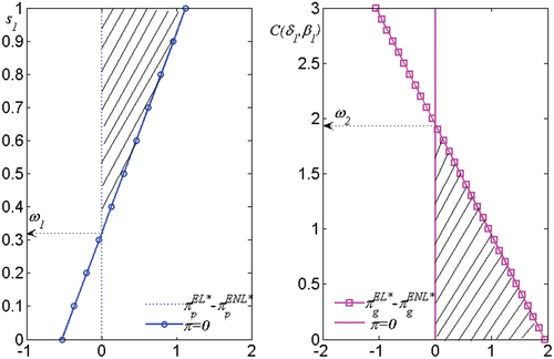
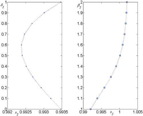
From Figure 11, in a certain range, with the growth of government subsidy for the producer’s PE reduction, the PE reduction effort of the producer will increase. Otherwise, the variable subsidy model is not feasible. The GPHL reduction subsidy coefficient for the producer has a positive relationship with the quality loss reduction coefficient of the producer and has a negative relationship with the quantity loss discount rate of the producer. In a certain range, with the growth of government subsidy for the producer’s GPHL reduction, the GPHL reduction effort of the producer will add.

Figure 11. Relationships between government subsidy and the efforts of producer (the loss reduction effort.

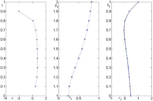
From Figure 12, in a certain range, the GPHL reduction subsidy coefficient for the retailer has a positive relationship with the retailer’s loss reduction coefficient about food quality and has a negative relationship with the quantity loss discount rate of the retailer. Based on these, in a certain range, government’s variable subsidy for the retailer’s GPHL reduction can encourage the producer to make post-harvest loss reduction effort.

Figure 12. Relationships between government subsidy and the retailer’s efforts (the loss reduction effort).

4.2. Robustness analyses

In this chapter, we will discuss the robustness of the proposed views. In the proposed models of ENL, EL and ELB, we only discussed the case of variable subsidies provided by the government. The government may provide mixed subsidy models such as variable subsidies and fixed subsidies. In China, the subsidy strategies used for agricultural pollution control include both fixed and variable subsidy models. For example, the subsidy for recycling agricultural film belongs to the variable subsidy model, and the support subsidy for green technology extension service has both fixed and variable subsidy modes (Chatterjee, 2018; Ricker-Gilbert & Jones, 2015). Thus, we will extend the proposed models of ENL, EL and ELB with the fixed subsidies $C_1$, $C_2$ and $C_3$ ($C_1$ presents the government fixed subsidy for the PE reduction cost, and $C_2$ is the government fixed subsidy for the producer’s loss reduction cost, and $C_3$ is the government fixed subsidy for the retailer’s loss reduction cost). The analysis process sees Appendix D. The results show that when the government only provides fixed subsidies, in the extended models (the models of DENL, DEL and DELB), the fixed subsidies ($C_1$, $C_2$ and $C_3$) have not an impact on the equilibrium price but have a positive impact on the income parameters of supply chain stakeholders. This result is like the result under the variable subsidy modes. These indicate that the model constructed by us has good robustness.

4.3. Discussion

Compared with the existing researches, our research results have the following differences.

1. In this study, we obtain that the environmental innovation subsidy coefficient will not influence the change trends of the equilibrium prices and the benefits of the retailer and government, this is different with the research results of Chen et al. (2017) and Zhang et al. (2020). It may be because in our paper, we improved the demand function and make it more suitable in dual context of PE reduction and PGHL reduction. In addition, the producer benefits will add, and this is same with the research results of Chen et al. (2017) and Zhang et al. (2020). In addition, when the environmental innovation subsidy coefficient and the PE reduction cost could meet a certain range, the producers’ PE reduction behavior and the government subsidy behavior will help chain members gain more benefits compared without adopting the environmental innovation technology. Our results are similar to the research results of Chen et al. (2017) and Zhang et al. (2020).

2. In this research, we also analyzed the effects of the effort level of PE reduction, the discount rate of the unit quantity loss, the quality loss reduction coefficient on equilibrium prices and benefits in the proposed four models; however, other studies (Cardoen et al., 2015; An & Ouyang, 2016; Gogh et al., 2017, Manivannan et al., 2017; Zhang et al., 2020) have not proposed and analyzed the impacts of these parameters on decision variables in the food supply chain. Thus, we will not discuss them.

3. Conclusions, significations, contributions and limitations

5. Conclusions, significations, contributions and limitations

5.1. Conclusions

This study aim is to understand the subsidy and investment rules of supply chain stakeholders under the PE reduction effort and the GPHL reduction effort. We firstly proposed concepts and function expressions of the reduction efforts on GPHL and PE. Finally, we proposed and analyzed four investment and subsidy models about the PE reduction and the food loss reduction and get some interesting findings.

(1) To achieve cleaner production in agriculture, the government should encourage producers to reduce PE. However, when the PE reduction cost is higher than a certain value, the variable subsidy model proposed in this paper is not feasible for government. In this case, the government can adopt the fixed subsidy strategies.

(2) No matter whether supply chain members invest in GPHL reduction technology or not, both the equilibrium prices and revenues of stakeholders have a positive relationship with the effort level of PE reduction.

(3) The GPHL reduction subsidy coefficients of the producer and retailer are only positively related to their own returns and are not related to the returns of other supply members. Even so, when the GPHL reduction subsidy coefficient and the loss reduction cost of the producer and the retailer meet a certain value, the adoption behaviors of the producer and the retailer about GPHL reduction technology can help supply chain members obtain better profits.

(4) No matter whether the producer or the retailer invests in GPHL reduction technology or not, both the equilibrium prices and revenues of stakeholders have a positive relationship with the quality loss reduction coefficient and have a negative relationship with the discount rate of the unit quantity loss. Namely, no matter whether the producer or the retailer invests in food loss reduction technology or not, both the equilibrium prices and revenues of stakeholders have a positive relationship with the loss reduction effort level of the producer or the retailer.

(5) Within a certain range, the government’s variable subsidies will motivate the producer and the retailer to reduce their post-harvest losses and PE.

5.2. Significations

The above research results have vital management significations and can offer some management decision help for food producers or other managers in the food supply chain. For instance, when the PE reduction cost is higher than a certain value, government should not adopt the variable subsidy model to subsidize the PE reduction behavior, and the government can adopt the fixed subsidy to encourage producers to implement environmentally innovative technologies and achieve cleaner production. In addition, if the producer and the government want to gain more benefits from investing in the GPHL reduction technology, they should pay attention to the value of mining GPHL reduction technology, and improve users’ GPHL reduction effort level as much as possible. Governments should also pay more attention to subsidize the GPHL reduction effort level rather than just the GPHL reduction costs. Subsidizing the GPHL reduction costs is easy, and subsidizing the GPHL reduction effort level needs to assess the GPHL reduction level. Government can entrust a third party or adopt blockchain or other technologies to monitor GPHL reduction level. Furthermore, government subsidy for the retailer’s loss reduction investment can increase the profit margin of the retailer. Meanwhile, the retailer should also try to reduce its loss reduction cost, only in this way, that government offers this varying subsidy model is feasible. From our research, we can also discover that the transport link of food from the producer to the retailer is a very important link in controlling the loss of food quality and quantity. If the retailer or producer wants to reduce the loss of food quality or quantity, the choice of transport enterprise or equipment is also very critical for them. From the perspective of food loss reduction, logistics enterprises or equipment with low transportation loss rate may be more popular in the future. Therefore, logistics managers should strive to improve their transportation efficiency and efficiency.

5.3. Contributions and limitations

In this section, to highlight our contributions, we compared this research with others (An & Ouyang, 2016; Cardoen et al., 2015; Chandrasekaran & Rajesh, 2017; Chen et al., 2017; Gogh et al., 2017; Zhang et al., 2020), and this research has the below differences.

1) Many studies disused effects of food GPHL on Agricultural PE (Cakar et al., 2020; Cattaneo et al., 2021; Huber et al., 2023; Ps et al., 2022; Tonini et al., 2018), and some existing researches focused on the agricultural PE and yield (Stathers et al., 2020), and few researchers consider GPHL reduction and agricultural PE reduction to explore government subsidy strategies and other members investment rules. Putting forward GPHL subsidy can encourage users adopt GPHL reduction equipment.

2) To obtain the relationships between GPHL reduction effort and government subsidy, according to the existing researches (Cardoen et al., 2015; An & Ouyang, 2016; Gogh et al., 2017; Chandrasekaran & Rajesh, 2017), we divided the GPHL into two categories: quantity loss and quality loss. We proposed the loss reduction level of grain quality and quantity and used them to reflect the GPHL reduction efforts of supply chain members in terms of quality and quantity.

3) In China, to carry out agricultural cleaner production, there are standards for controlling agricultural PE,⁵ in this paper, we assume a maximum value of the allowable PE $M$ and a unit PE of food producer $e_0$ to express the maximum output $M/e_0$ under PE limits. In addition, Chinese food supply and demand have been in tight balance for a long time, and we put forward that the output equals the demand. Compared with the existing researches (Chen et al., 2017; Zhang et al., 2020), our research hypothesis is more realistic. Based on these and considering the effects of supply chain members’ loss reduction efforts on food quality decay, we revised the market demand.

There are some limitations in this paper. (1) Firstly, the method we adopt is Stackelberg game, and it is one in which the players know each other’s returns and they all know exactly what is going on before they choose. We use the master-slave game model as the main model, which mainly describes the content of the duopoly game model and is a dynamic game model with complete information sharing, aiming to solve the problem of market economy. However, in reality, the information among supply chain members is not equal, and the master-slave game under asymmetric information may be closer to reality. (2) Although we considered food output subsidy, we did not discuss the coupling relationship between the output subsidy and other subsidies. In the next research, we will focus on the coupling relationship between the output subsidy and the loss reduction subsidy. In addition, we only discussed the case of variable subsidies provided by the government. The government may provide mixed subsidy models such as variable subsidies and fixed subsidies. In the next research, we will focus on this issue. We also proposed that to stimulate food enterprises or producers to more effectively reduce GPHL, the government should subsidize the GPHL reduction effort level of food enterprises. However, we have not made an in-depth study on the subsidy mechanism, and we can also make an in-depth discussion on this aspect in the future.

Author’s Contributions

Pan Liu, Changxia Sun, Bingjun Li and Mengjuan Li conceived and designed the experiments, analyzed the data and wrote the paper.

Disclosure statement

No potential conflict of interest was reported by the author(s).

Additional information

Funding

This work was partially supported by Top Talent Project of Henan Agricultural University (No. 30500681), and Creator Talent Support Plan of Henan Agricultural University (No. 30200757), and Humanities and Social Science Research Youth Project of the Education Ministry of China (No.21YJC790076), Postdoctoral Science Foundation (2022M721039), and Henan University Philosophy and Social Science Innovation Talent Support Program (No. 2023-CXRC-24).

Notes

1. http://www.moa.gov.cn/and http://www.lswz.gov.cn/

2. https://data.stats.gov.cn/easyquery.htm?cn =C01&zb =A0C 03&sj = 2021

3. http://www.npc.gov.cn/npc/c30834/202012/54c3e0f5e7e94ecab9feb5cf9f522f25.shtml

4. https://www.66law.cn/laws/597266.aspx

5. (https://www.mee.gov.cn/gkml/hbb/bgg/201010/t20101022_196441.htm

Appendix A

Proof.

Based on Assumptions (6), we know that in the NEL model$D^{NEL}=M/M{e}_0-x{e}_0$, and putting it into formula (2), solving the first partial derivative of ${\pi }_r^{NEL}$ with respect to $p^{NEL}$ and let it equal to zero, we can get $p^{NEL}(w^{NEL})$. Then, putting $p^{NEL}(w^{NEL})$ into formula (1), solving the first partial derivative of ${\pi }_p^{NEL}$ with respect to $w^{NEL}$ and let it equal to zero, we can get $w^{NEL\ast }$. Based on $w^{NEL\ast }$ and $p^{NEL}(w^{NEL})$, we can get $p^{NEL\ast }$. According to $w^{NEL\ast }$ and $p^{NEL\ast }$, we can get ${\pi }_r^{NEL\ast }$, ${\pi }_p^{NEL\ast }$ and ${\pi }_g^{NEL\ast }$.

Appendix B

According to proposition 2, we can get $\frac{\mathrm{\partial }{p}^{ENL\ast }}{\mathrm{\partial }s}=0$, $\frac{\mathrm{\partial }{w}^{ENL\ast }}{\mathrm{\partial }s}=0$, $\frac{\mathrm{\partial }{\pi }_r^{ENL\ast }}{\mathrm{\partial }s}=0$, $\frac{\mathrm{\partial }{\pi }_p^{ENL\ast }}{\mathrm{\partial }s}=\frac{k{\gamma }^2}{2}>0$ and $\frac{\mathrm{\partial }{\pi }_g^{ENL\ast }}{\mathrm{\partial }s}=0$. $\frac{\mathrm{\partial }{p}^{ENL\ast }}{\mathrm{\partial }\gamma }=\frac{3M}{4e_0{(1-\gamma )}^2}>0$, $\frac{\mathrm{\partial }{w}^{ENL\ast }}{\mathrm{\partial }\gamma }=\frac{M}{2e_0{(1-\gamma )}^2}>0$, $\frac{\mathrm{\partial }{\pi }_r^{ENL\ast }}{\mathrm{\partial }\gamma }=\frac{(1-{\lambda }_1)(1-{\lambda }_2)E}{8{({\mathrm{e}}_0)}^2{(1-\gamma )}^3}>0$, $\frac{\mathrm{\partial }{\pi }_p^{ENL\ast }}{\mathrm{\partial }\gamma }=$$\frac{(1-{\lambda }_1)E^2+(1-s)k\gamma }{4{({\mathrm{e}}_0)}^2{(1-\gamma )}^3}-\frac{(1-{\lambda }_1)(\beta -c-q_0(1-{\alpha }_1-{\alpha }_2+{\alpha }_1{\alpha }_2))E}{4{\mathrm{e}}_0{(1-\gamma )}^2}>0$. $\frac{\mathrm{\partial }{\pi }_g^{ENL\ast }}{\mathrm{\partial }\gamma }=\frac{\mathrm{\partial }{\pi }_r^{ENL\ast }}{\mathrm{\partial }\gamma }+\frac{\mathrm{\partial }{\pi }_p^{ENL\ast }}{\mathrm{\partial }\gamma }+\frac{\mathrm{\partial }C{S}_{\hspace{0.17em}}^{ENL\ast }}{\mathrm{\partial }\gamma }-\frac{\mathrm{\partial }{D}^{ENL\ast }}{\mathrm{\partial }\gamma }-skr$, Due to $\frac{\mathrm{\partial }{\pi }_r^{ENL\ast }}{\mathrm{\partial }\gamma }=\frac{(1-{\lambda }_1)(1-{\lambda }_2)E}{8{({\mathrm{e}}_0)}^2{(1-\gamma )}^3}$, $\frac{\mathrm{\partial }{\pi }_p^{ENL\ast }}{\mathrm{\partial }\gamma }=\frac{(1-{\lambda }_1)E^2+(1-s)k\gamma }{4{({\mathrm{e}}_0)}^2{(1-\gamma )}^3}-\frac{(1-{\lambda }_1)(\beta -c-q_0(1-{\alpha }_1-{\alpha }_2+{\alpha }_1{\alpha }_2))E}{4{\mathrm{e}}_0{(1-\gamma )}^2}$, $\frac{\mathrm{\partial }C{S}_{\hspace{0.17em}}^{ENL\ast }}{\mathrm{\partial }\gamma }=$$\frac{ME}{16{({\mathrm{e}}_0)}^2{(1-\gamma )}^3}$ and $\frac{\mathrm{\partial }{D}^{ENL\ast }}{\mathrm{\partial }\gamma }=\frac{\beta M}{4e_0{(1-\gamma )}^2}$, $\frac{\mathrm{\partial }{\pi }_g^{ENL\ast }}{\mathrm{\partial }\gamma }>0$. Thus, we can get Inference 1.

Appendix C

Appendix

Proof.

If ${\pi }_p^{ENL\ast }\ge {\pi }_p^{NEL\ast }$, the producer will adopt the PE reduction technology; therefore, we get $s>1-\frac{(1-{\lambda }_1)M\{(2-\gamma )M+2(1-\gamma )[e_0{q}_0(1-{\alpha }_1-{\alpha }_2+{\alpha }_1{\alpha }_2)+e_0(\beta -c)]\}}{4\gamma k{(e_0)}^2}$, we call it $s>{\psi }_1$. If ${\pi }_g^{ENL\ast }\ge {\pi }_g^{NEL\ast }$, subsidizing the PE reduction investment of the producer, government will get more social benefit; therefore, we can get $\frac{[2(1-{\lambda }_1)(1-{\lambda }_2)+4(1-{\lambda }_1)+1][E^2-A^2{(1-\gamma )}^2]}{32{(e_0)}^2{(1-\gamma )}^2}-\frac{\beta \gamma M}{4e_0(1-\gamma )}>\frac{k{\gamma }^2}{2}$, we call it $C(\gamma )<{\psi }_2$. If ${\pi }_p^{ENL\ast }\ge {\pi }_p^{NEL\ast }$ and ${\pi }_g^{ENL\ast }\ge {\pi }_g^{NEL\ast }$, for the producer and the government, investing in the PE reduction technology and subsidizing this investment is feasible. Namely, when $s>{\psi }_1$ and $C(\gamma )<{\psi }_2$ can be met, investing in the PE reduction technology and subsidizing this investment is feasible.

Appendix

Proof.

If ${\pi }_p^{EL\ast }\ge {\pi }_p^{ENL\ast }$, the producer will adopt the PE reduction technology, at the same time, he/she will adopt the GPHL reduction technology, and we get $s_1>1-\frac{(1-{\delta }_1{\lambda }_1)E_1^2-(1-{\lambda }_1)E^2}{4{(e_0)}^2{(1-\gamma )}^2[k_1{(1-{\delta }_1)}^2+k_2{({\beta }_1-1)}^2]}$, it is called $s_1>{\zeta }_1$. If ${\pi }_g^{EL\ast }\ge {\pi }_g^{ENL\ast }$, subsidizing the PE reduction investment and the loss reduction inputs of the producer, government will get more social benefit, and we can get $\frac{E_1^2[2(1-{\delta }_1{\lambda }_1)(1-{\lambda }_2)+4(1-{\lambda }_1)+1]-E_{\hspace{0.17em}}^2[2(1-{\lambda }_1)(1-{\lambda }_2)+4(1-{\lambda }_1)+1]}{32{(e_0)}^2{(1-\gamma )}^2}-\frac{\beta (E_1-E_{\hspace{0.17em}})}{4e_0(1-\gamma )}>\frac{k_2{(1-{\beta }_1)}^2+k_1{(1-{\delta }_1)}^2}{2}$, and it is called $C({\delta }_1,{\beta }_1)<{\zeta }_2$. If ${\pi }_p^{ENL\ast }\ge {\pi }_p^{NEL\ast }$ and ${\pi }_g^{ENL\ast }\ge {\pi }_g^{NEL\ast }$, for the producer and the government, investing in the PE reduction technology and subsidizing this investment is feasible. Namely, when $s_1>{\zeta }_1$ and $C({\delta }_1,{\beta }_1)<{\zeta }_2$, investing in the PE reduction technology and subsidizing this investment is feasible.

Appendix

Proof.

If ${\pi }_r^{ELB\ast }\ge {\pi }_r^{EL\ast }$, the retailer will adopt the GPHL reduction technology, and we get that $s_2>1-\frac{(1-{\delta }_1{\lambda }_1)(1-{\delta }_2{\lambda }_2)E_2^2-(1-{\delta }_1{\lambda }_1)(1-{\lambda }_2)E_1^2}{8{(e_0)}^2{(1-\gamma )}^2[k_4{(1-{\delta }_2)}^2+k_3{({\beta }_2-1)}^2]}$, and it is called $s_2>{\xi }_1$. If ${\pi }_g^{ELB\ast }\ge {\pi }_g^{EL\ast }$, subsidizing the loss reduction inputs of the retailer, government will get more social benefits, and we can get $\frac{E_2^2[2(1-{\delta }_1{\lambda }_1)(1-{\delta }_2{\lambda }_2)+4(1-{\lambda }_1)+1]-E_1^2[2(1-{\delta }_1{\lambda }_1)(1-{\lambda }_2)+4(1-{\lambda }_1)+1]}{32{(e_0)}^2{(1-\gamma )}^2}-\frac{\beta (E_2-E_1)}{4e_0(1-\gamma )}>\frac{k_3{(1-{\beta }_2)}^2+k_4{(1-{\delta }_2)}^2}{2}$, and it is called $C({\delta }_2,{\beta }_2)<{\xi }_2$. If ${\pi }_p^{ELB\ast }\ge {\pi }_p^{NL\ast }$ and ${\pi }_g^{ELB\ast }\ge {\pi }_g^{NL\ast }$, for the producer and the government, investing in the PE reduction technology and subsidizing this investment is feasible. When $s_2>{\xi }_1$ and $\mathrm{C}({\delta }_2,{\beta }_2)<{\xi }_2$, investing in the PE reduction technology and subsidizing this investment is feasible.

Appendix D

In the DENL model, Revenues’ functions of the food producer, the retailer and government are as follows: ${\pi }_p^{ENL}=(w^{ENL}-c+\beta )D^{ENL}(1-{\lambda }_1)-\frac{k{\gamma }^2}{2}+C_1$, ${\pi }_r^{ENL}=(p^{ENL}-w^{ENL})D^{ENL}(1-{\lambda }_1)(1-{\lambda }_2)$ and ${\pi }_g^{ENL}={\pi }_p^{ENL}+{\pi }_r^{ENL}+C{S}^{ENL}-\beta D^{ENL}-\frac{k{\gamma }^2}{2}-C_1$ Based on these, the optimal decision about the retail price, the effort level of PE reduction, benefits of the food producer and government are as follows.$\left\{\begin{array}{c}{w}^{ENL\ast }=-\frac{(\beta -c)}{2}-B\\ p^{ENL\ast }=\frac{\beta -c}{4}-\frac{3B}{2}\\ D_{\hspace{0.17em}}^{NEL\ast }=\frac{E}{4{\mathrm{e}}_0(1-\gamma )}\end{array}\right.$ $\left\{\begin{array}{c}{\pi }_p^{ENL\ast }=\frac{(1-{\lambda }_1)E^2}{8{(e_0)}^2{(1-\gamma )}^2}-\frac{k{\gamma }^2}{2}+C_1\\ {\pi }_r^{ENL\ast }=\frac{(1-{\lambda }_1)(1-{\lambda }_2)E^2}{16{(e_0)}^2{(1-\gamma )}^2}\\ {\pi }_g^{ENL\ast }=\frac{E^2[(1-{\lambda }_1)(1-{\lambda }_2)+2(1-{\lambda }_1)+2]}{32{(e_0)}^2{(1-\gamma )}^2}-\frac{k{\gamma }^2}{2}-\frac{\beta E}{4e_0(1-\gamma )}-C_1\end{array}\right.$

According to these and Chapter 5, we get the fixed subsidy $C_1$ has not an impact on the equilibrium price, but has a positive impact on the income parameters of the producer and has a negative impact on the government’s revenue.

The calculation process in the models of DEL and DELB is similar to those in the DENL model; here, it will not be described.

References

- Allaoui, H., Guo, Y., Choudhary, A., & Bloemhof, J. (2018). Sustainable agro-food supply chain design using two-stage hybrid multi-objective decision-making approach. Computers & Operations Research, 89, 369–28. https://doi.org/10.1016/j.cor.2016.10.012
- Amiri, A. (2006). Designing a distribution network in a supply chain system: Formulation and efficient solution procedure. European Journal of Operational Research, 171(2), 567–576. https://doi.org/10.1016/j.ejor.2004.09.018
- An, K., & Ouyang, Y. (2016). Robust grain supply chain design considering post-harvest loss and harvest timing equilibrium. Transportation Research Part E, 88(april), 110–128. https://doi.org/10.1016/j.tre.2016.01.009
- Bendinelli, W. E., Su, C. T., Pera, T. G., & Caixeta-Filho, J. V. (2019). What are the main factors that determine post-harvest losses of grains? Sustainable Production and Consumption, 21, 228–238. https://doi.org/10.1016/j.spc.2019.09.002
- Caixeta-Filho, J. V., & Pera, T. G. (2018). Post-harvest losses during the transportation of grains from farms to aggregation points. International Journal of Logs Economics & Globalisation, 7(3), 209–247. https://doi.org/10.1504/IJLEG.2018.093755
- Cakar, B., Aydin, S., Varank, G., & Al, E. (2020). Assessment of environmental impact of FOOD waste in Turkey. Journal of Cleaner Production, 244, 118846. https://doi.org/10.1016/j.jclepro.2019.118846
- Cardoen, D., Joshi, P., Diels, L., Sarma, P. M., & Pant, D. (2015). Agriculture biomass in India: Part 2. Post-harvest losses, cost and environmental impacts. Resources Conservation & Recycling, 101, 143–153. https://doi.org/10.1016/j.resconrec.2015.06.002
- Cattaneo, A., Federighi, G., & Vaz, S. (2021). The environmental impact of reducing food loss and waste: A critical assessment. Food Policy, 98, 101890. https://doi.org/10.1016/j.foodpol.2020.101890
- Chandrasekaran, M., & Rajesh, R. (2017). Modelling and optimisation of Indian traditional agriculture supply chain to reduce post-harvest loss and CO2 emission. Industrial Management & Data Systems, 117(9), 1817–1841. https://doi.org/10.1108/IMDS-09-2016-0383
- Chatterjee, S. (2018). Storage infrastructure and agricultural yield: Evidence from a capital investment subsidy scheme. Economics, 12(1), 1–20. https://doi.org/10.5018/economics-ejournal.ja.2018-65
- Chen, S. P., & Chen, C. Y. (2020). Dynamic markdown decisions based on a quality loss function in on-site direct-sale supply chains for perishable food. Journal of the Operational Research Society, 72(4), 822–836. https://doi.org/10.1080/01605682.2019.1705192
- Chen, J. Y., Dimitrov, S., & Pun, H. (2019). The impact of government subsidy on supply chains’ sustainability innovation. Omega, 86, 42–58. https://doi.org/10.1016/j.omega.2018.06.012
- Cheng, L. L., Yin, C. B., Hu, W. L., & Zhou, Y. (2011). Subsidy policy for agricultural nonpoint pollution control in northern area of Erhai Lake of Yunnan province. Agro-Environment & Development, 31(4), 471–474.
- Chen, Y., Miao, J., & Zhu, Z. (2021). Measuring green total factor productivity of China’s agricultural sector: A three-stage SBM-DEA model with non-point source pollution and CO 2 emissions. Journal of Cleaner Production, 318, 127934. https://doi.org/10.1016/j.jclepro.2021.128543
- Chen, Y. H., Wen, X. W., Wang, B., & Nie, P. Y. (2017). Agricultural pollution and regulation: How to subsidize agriculture? Journal of Cleaner Production, 164(oct.15), 258–264. https://doi.org/10.1016/j.jclepro.2017.06.216
- China, N. F. A. S. (2020). How to reduce post-production loss of grain June 27, 2022, from http://www.lswz.gov.cn/html/zt/kjhdz2021/2021-06/09/content_266101.shtml
- Do Rosário Cameira, M., Rolim, J., Valente, F., Mesquita, M., Dragosits, U., & Cordovil, C. M. (2021). Translating the agricultural N surplus hazard into groundwater pollution risk: Implications for effectiveness of mitigation measures in nitrate vulnerable zones. Agriculture, Ecosystems and Environment, 306, 107204. https://doi.org/10.1016/j.agee.2020.107204
- Duan, C., Yao, F., Guo, X. E. A., Yu, H., & Wang, Y. (2022). The impact of carbon policies on supply chain network equilibrium: Carbon trading price, carbon tax and low-carbon product subsidy perspectives. International Journal of Logistics: Research & Applications, 1–25. https://doi.org/10.1080/13675567.2022.2122422
- FAO. (2013). Food wastage footprint; impacts on natural resources (summary report), from http://www.fao.org/docrep/018/i3347e/i3347e.pdf
- Gitonga, Z. M., Groote, H. D., Kassie, M., & Tefera, T. (2013). Impact of metal silos on households’ maize storage, storage losses and food security: An application of a propensity score matching. Food Policy, 43, 44–55. https://doi.org/10.1016/j.foodpol.2013.08.005
- Gogh, B. V., Boerrigter, H., Noordam, M., Ruben, R., & Timmermans, T. (2017). Post-harvest loss reduction. Wageningen Food & Biobased Research.
- Gunasekera, D., Parsons, H., & Smith, M. (2017). Post-harvest loss reduction in Asia-Pacific developing economies. Journal of Agribusiness in Developing and Emerging Economies, 7(3), 303–317. https://doi.org/10.1108/JADEE-12-2015-0058
- He, P., He, Y., & Xu, H. (2021). Channel structure and pricing in a dual-channel closed-loop supply chain with government subsidy. International Journal of Production Economics, 213, 108–123. https://doi.org/10.1016/j.ijpe.2019.03.013
- Hengsdijk, H., & Boer, W. D. (2017). Post-harvest management and post-harvest losses of cereals in Ethiopia. Food Security, 9(5), 945–958. https://doi.org/10.1007/s12571-017-0714-y
- Hodges, R. J., Buzby, J. C., & Bennett, B. (2011). Postharvest losses and waste in developed and less developed countries: Opportunities to improve resource use. The Journal of Agricultural Science, 149(s1), 37–45. https://doi.org/10.1017/S0021859610000936
- Huang, S., Fan, Z. P., & Wang, N. (2020). Green subsidy modes and pricing strategy in a capital-constrained supply chain. Transportation Research Part E: Logistics & Transportation Review, 136, 101885. https://doi.org/10.1016/j.tre.2020.101885
- Huang, H., He, Y., & Li, D. (2018). Pricing and inventory decisions in the food supply chain with production disruption and controllable deterioration. Journal of Cleaner Production, 180, 280–296. https://doi.org/10.1016/j.jclepro.2018.01.152
- Huber, R., Tarruella, M., & Hansen, J. W. E. A. (2023). Marginal climate change abatement costs in Swiss dairy production considering farm heterogeneity and interaction effects. Agricultural Systems, 207, 103639. https://doi.org/10.1016/j.agsy.2023.103639
- Jiang, Y., Li, K., Chen, S. E. A., Fu, X., Feng, S., & Zhuang, Z. (2022). A sustainable agricultural supply chain considering substituting organic manure for chemical fertilizer. Sustainable Production and Consumption, 29, 432–446. https://doi.org/10.1016/j.spc.2021.10.025
- Julian, P., Mark, B., & Sarah, M. (2018). Food waste within food supply chains: Quantification and potential for change to 2050. Philosophical Transactions of the Royal Society of London: Series B, Biological Sciences, 365(1554), 3065–3081. https://doi.org/10.1098/rstb.2010.0126
- Kaminski, J., & Christiaensen, L. (2014). Post-harvest loss in sub-saharan Africa—what do farmers say? Global Food Security, 3(3–4), 149–158. https://doi.org/10.1016/j.gfs.2014.10.002
- Khan, S. A. R., Ahmad, Z., Sheikh, A. A. E. A., & Yu, Z. (2022). Digital transformation, smart technologies, and eco-innovation are paving the way toward sustainable supply chain performance. Science Progress, 105(4), 1–26. https://doi.org/10.1177/00368504221145648
- Khan, S. A. R., Tabish, M., & Zhang, Y. (2023). Embracement of industry 4.0 and sustainable supply chain practices under the shadow of practice-based view theory: Ensuring environmental sustainability in corporate sector. Journal of Cleaner Production, 398, 136609. https://doi.org/10.1016/j.jclepro.2023.136609
- Khan, S. A. R., Zhang, Y., & Farooq, K. (2023). Green capabilities, green purchasing, and triple bottom line performance: Leading toward environmental sustainability. Business Strategy and the Environment, 32(4), 2022–2034. https://doi.org/10.1002/bse.3234
- Kuiper, M., & Cui, H. D. (2021). Using food loss reduction to reach food security and environmental objectives - a search for promising leverage points. Food Policy, 98, 101915. https://doi.org/10.1016/j.foodpol.2020.101915
- Li, S., He, Y., & Salling, M. (2021). Strategic rationing and freshness keeping of perishable products under transportation disruptions and demand learning. Complex & Intelligent Systems, 8(6), 1–15. https://doi.org/10.1007/s40747-021-00492-w
- Li, H., Tang, M., & Cao, A. E. A. (2022). Assessing the relationship between air pollution, agricultural insurance, and agricultural green total factor productivity: Evidence from China. Environmental Science and Pollution Research, 29(52), 1–15. https://doi.org/10.1007/s11356-022-21287-7
- Liu, P. (2019). Pricing policies and coordination of low-carbon supply chain considering targeted advertisement and carbon emission reduction costs in the big data environment. Journal of Cleaner Production, 210(FEB.10), 343–357. https://doi.org/10.1016/j.jclepro.2018.10.328
- Liu, L., Ouyang, W., Liu, H., Zhu, J., Fan, X., Zhang, F., Ma, Y., Chen, J., Hao, F., & Lian, Z. (2021). Drainage optimization of paddy field watershed for diffuse phosphorus pollution control and sustainable agricultural development. Agriculture, Ecosystems & Environment, 308(3), 107238. https://doi.org/10.1016/j.agee.2020.107238
- Li, B., Yin, T., Udugama, I. A., & Al, E. (2020). Food waste and the embedded phosphorus footprint in China. Journal of Cleaner Production, 252, 119909. https://doi.org/10.1016/j.jclepro.2019.119909
- Lu, Y., Song, S., Wang, R., Liu, Z., Meng, J., Sweetman, A. J., & Luo, W. (2015). Impacts of soil and water pollution on food safety and health risks in China. Environment International, 77(april), 5–15. https://doi.org/10.1016/j.envint.2014.12.010
- Lu, X., Ye, X., Zhou, M. E. A., Zhao, Y., Weng, H., Kong, H., Li, K., Gao, M., Zheng, B., Lin, J., Zhou, F., Zhang, Q., Wu, D., Zhang, L., & Zhang, Y. (2021). The underappreciated role of agricultural soil nitrogen oxide emissions in ozone pollution regulation in North China. Nature Communications, 12(1), 1–9. https://doi.org/10.1038/s41467-021-25147-9
- Ma, S., He, Y., Gu, R. E. A., & Li, S. (2021). Sustainable supply chain management considering technology investments and government intervention. Transportation Research Part E: Logistics & Transportation Review, 149, 102290. https://doi.org/10.1016/j.tre.2021.102290
- Majiwa, E., Lee, B. L., Wilson, C. E. A., Fujii, H., & Managi, S. (2018). A network data envelopment analysis (NDEA) model of post-harvest handling: The case of Kenya’s rice processing industry. Food Security, 10(3), 631–648. https://doi.org/10.1007/s12571-018-0809-0
- Ma, X., Wang, J., Bai, Q., & Wang, S. (2019). Optimization of a three-echelon cold chain considering freshness-keeping efforts under cap-and-trade regulation in industry 4.0. International Journal of Production Economics, 220, 107457. https://doi.org/10.1016/j.ijpe.2019.07.030
- Ma, W., Zhao, Z., & Ke, H. (2013). Dual-channel closed-loop supply chain with government consumption-subsidy. European Journal of Operational Research, 226(2), 221–227. https://doi.org/10.1016/j.ejor.2012.10.033
- Meng, Q., Li, M., & Liu, W. E. A. (2021). Pricing policies of dual-channel green supply chain: Considering government subsidies and consumers’ dual preferences. Sustainable Production and Consumption, 26, 1021–1030. https://doi.org/10.1016/j.spc.2021.01.012
- Mishra, R. K., Mohammad, N., & Roychoudhury, N. (2016). Soil pollution: Causes, effects and control. Van Sangyan, 3(1), 1–14.
- Mogale, D. G., Kumar, S. K., & Tiwari, M. K. (2020). Green food supply chain design considering risk and post-harvest losses: A case study. Annals of Operations Research, 295(1), 257–284. https://doi.org/10.1007/s10479-020-03664-y
- Nie, P. (2012). A monopoly with pollution emissions. Journal of Environmental Planning and Management, 55(6), 705–711. https://doi.org/10.1080/09640568.2011.622742
- Nourbakhsh, S. M., Bai, Y., Maia, G., Ouyang, Y., & Rodriguez, L. (2016). Grain supply chain network design and logistics planning for reducing post-harvest loss. Biosystems Engineering, 151, 105–115. https://doi.org/10.1016/j.biosystemseng.2016.08.011
- Olorunfemi, B. J., & Kayode, S. E. (2021). Post-harvest loss and grain storage technology- a review. Turkish Journal of Agriculture - Food Science & Technology, 9(1), 75–83. https://doi.org/10.24925/turjaf.v9i1.75-83.3714
- Omotilewa, O. J., Jacob, R. G., Herbert, A. J., & Shively, G. E. (2018). Does improved storage technology promote modern input use and food security? Evidence from a randomized trial in Uganda. Journal of Development Economics, 135, 176–198. https://doi.org/10.1016/j.jdeveco.2018.07.006
- Panchasara, H., Samrat, N. H., & Islam, N. G. G. E. (2021). Greenhouse gas emissions trends and mitigation measures in Australian agriculture sector—A review. Agriculture, 11(2), 11020085. https://doi.org/10.3390/agriculture11020085
- Parris, K. (2011). Impact of agriculture on water pollution in OECD countries: Recent trends and future prospects. International Journal of Water Resources Development, 27(1), 33–52. https://doi.org/10.1080/07900627.2010.531898
- Peng, H., & Pang, T. (2019). Optimal strategies for a three-level contract-farming supply chain with subsidy. International Journal of Production Economics, 216, 274–286. https://doi.org/10.1016/j.ijpe.2019.06.011
- Ps, A., Htb, A., Sm, A., & Lra, B. (2022). Biofertilization of biogas digestates: An insight on nutrient management, soil microbial diversity and greenhouse gas emission. New and Future Developments in Microbial Biotechnology and Bioengineering, 199–215. https://doi.org/10.1016/B978-0-323-85579-2.00002-2
- Qiao, H., Zheng, F., Jiang, H., & Dong, K. (2019). The greenhouse effect of the agriculture-economic growth-renewable energy nexus: Evidence from G20 countries. Science of the Total Environment, 671(25), 722–731. https://doi.org/10.1016/j.scitotenv.2019.03.336
- Ricker-Gilbert, J., & Jones, M. (2015). Does storage technology affect adoption of improved maize varieties in Africa? Insights from Malawi’s input subsidy program. Food Policy, 50, 92–105. https://doi.org/10.1016/j.foodpol.2014.10.015
- Sazvar, Z., Rahmani, M., & Govindan, K. (2018). A sustainable supply chain for organic, conventional agro-food products: The role of demand substitution, climate change and public health. Journal of Cleaner Production, 194, 564–583. https://doi.org/10.1016/j.jclepro.2018.04.118
- Shuanwang, Q., Ziqun, W., Hongxia, X., Wuzhou, G., & Baoguo, M. (2022). Estimation and analysis of agricultural non-point source pollution in Handan of Haihe River Basin. Journal of Hebei University of Engineering, 39(2), 86–92.
- Stathers, T., Holcroft, D., Kitinoja, L., Mvumi, B. M., English, A., Omotilewa, O., Kocher, M., Ault, J., & Torero, M. (2020). A scoping review of interventions for crop postharvest loss reduction in sub-saharan Africa and South Asia. Nature Sustainability, 3(10), 821–835. https://doi.org/10.1038/s41893-020-00622-1
- Sun, L., Cao, X., Alharthi, M., Zhang, J., Taghizadeh-Hesary, F., & Mohsin, M. (2016). Carbon emission transfer strategies in supply chain with lag time of emission reduction technologies and low-carbon preference of consumers - ScienceDirect. Journal of Cleaner Production, 264, 121664. https://doi.org/10.1016/j.jclepro.2020.121664
- Tadesse, M. (2020). Post-harvest loss of stored grain, its causes and reduction strategies. Food Science and Quality Management, 96, 26–35. https://doi.org/10.7176/FSQM/96-04
- Tonini, D., Albizzati, P. F., & Astrup, T. F. (2018). Environmental impacts of food waste: Learnings and challenges from a case study on UK. Waste Management, 76, 744–766. https://doi.org/10.1016/j.wasman.2018.03.032
- Vermeulen, S. J. C. B., Campbell, B. M., & Ingram, J. S. I. (2012). Climate change and food systems. Annual Review of Environment and Resources, 37(1), 195–222. https://doi.org/10.1146/annurev-environ-020411-130608
- Wang, W., Lin, W., & Cai, J. E. A. (2021). Impact of demand forecast information sharing on the decision of a green supply chain with government subsidy. Annals of Operations Research, 1–26. https://doi.org/10.1007/s10479-021-04233-7
- Wikström, F., Williams, H., & Venkatesh, G. (2016). The influence of packaging attributes on recycling and food waste behaviour–an environmental comparison of two packaging alternatives. Journal of Cleaner Production, 137, 895–902. https://doi.org/10.1016/j.jclepro.2016.07.097
- Zhang, J. B. (2023). Improving inherent soil productivity underpins agricultural sustainability. Pedosphere, 33(1), 3–5. https://doi.org/10.1016/j.pedsph.2023.01.007
- Zhang, C., Liu, S., Wu, S., Jin, S., Reis, S., Liu, H., & Gu, B. (2019). Rebuilding the linkage between livestock and cropland to mitigate agricultural pollution in China. Resources Conservation & Recycling, 144, 65–73. https://doi.org/10.1016/j.resconrec.2019.01.011
- Zhang, R., Ma, W., & Liu, J. (2020). Impact of government subsidy on agricultural production and pollution: A game-theoretic approach. Journal of Cleaner Production, 285, 124806. https://doi.org/10.1016/j.jclepro.2020.124806
- Zorya, S., Morgan, N., & Dia, Z. R. L. E. (2011). Missing food: The case of postharvest grain losses in Sub-Saharan Africa. The World Bank.